Filter pruning - deeper layers need fewer filters

Abstract

Model pruning aims to reduce the parameter amount of deep neural networks while retaining the performance. Existing strategies often treat all layers equally and all layers simply share the same pruning rate. However, it is observed from our experiments that the redundancy degree differs from layer to layer. Based on this observation, this work proposes a pruning strategy depending on the layer-wise redundancy degree. Firstly, we define the redundancy degree for each layer by the norm and similarity redundancy of filters. Then a novel layer-wise strategy, Redundancy-dependent Filter Pruning (RedFiP), is proposed which prunes different proportion of filters at different layers according to the defined redundancy degree. Since the redundancy analysis and experimental results of RedFiP show that deeper layers need fewer filters, a phase-wise strategy, Phased Filter Pruning (PFP), is proposed that divides the layers into three phases and layers in each phase share the same pruning rate. The phase-wise PFP allows the layer-wise RedFiP to be easily implemented in existing structures of deep neural networks. Experimental results show that when total parameters are pruned by 40%, RedFiP outperforms the state-of-the-art strategy FPGM-Mixed by 1.83% on CIFAR-100, and even slightly outperforms the non-pruned model by 0.11% on CIFAR-10. On ImageNet-1k, RedFiP (30%) and PFP (30%) outperform FPGM-Mixed (30%) by 1.3% and 0.8% with ResNet-18.

Keywords

Filter pruning redundancy phase importance

1 Introduction

Deep convolutional neural networks (CNNs) have been widely applied in many computer vision fields including face recognition, object detection, instance segmentation, etc. In general, CNNs containing more layers and/or kernels have a stronger feature learning representation ability, and hence perform better on many tasks, such as image classification and object detection. A variety of deeper and wider architectures [1 –3] have been designed for better feature learning representation ability [4 –6]. In these architectures, two hyperparameters are often manually set: the number of convolutional layers and the number of filters at each layer, i.e., the width and depth of the deep models. Since deeper and wider models generally have a better generalization, both parameters tend to be manually set to larger numbers.

Nevertheless, many reported results show that an excessive number of parameters are actually not necessitated, i.e., part of parameters are redundant and of little importance for extracting meaningful features. Denil et al. [7] demonstrated that there is significant redundancy in CNNs which are over-parameterized. For example, ReLU converts some units of feature maps to zero. 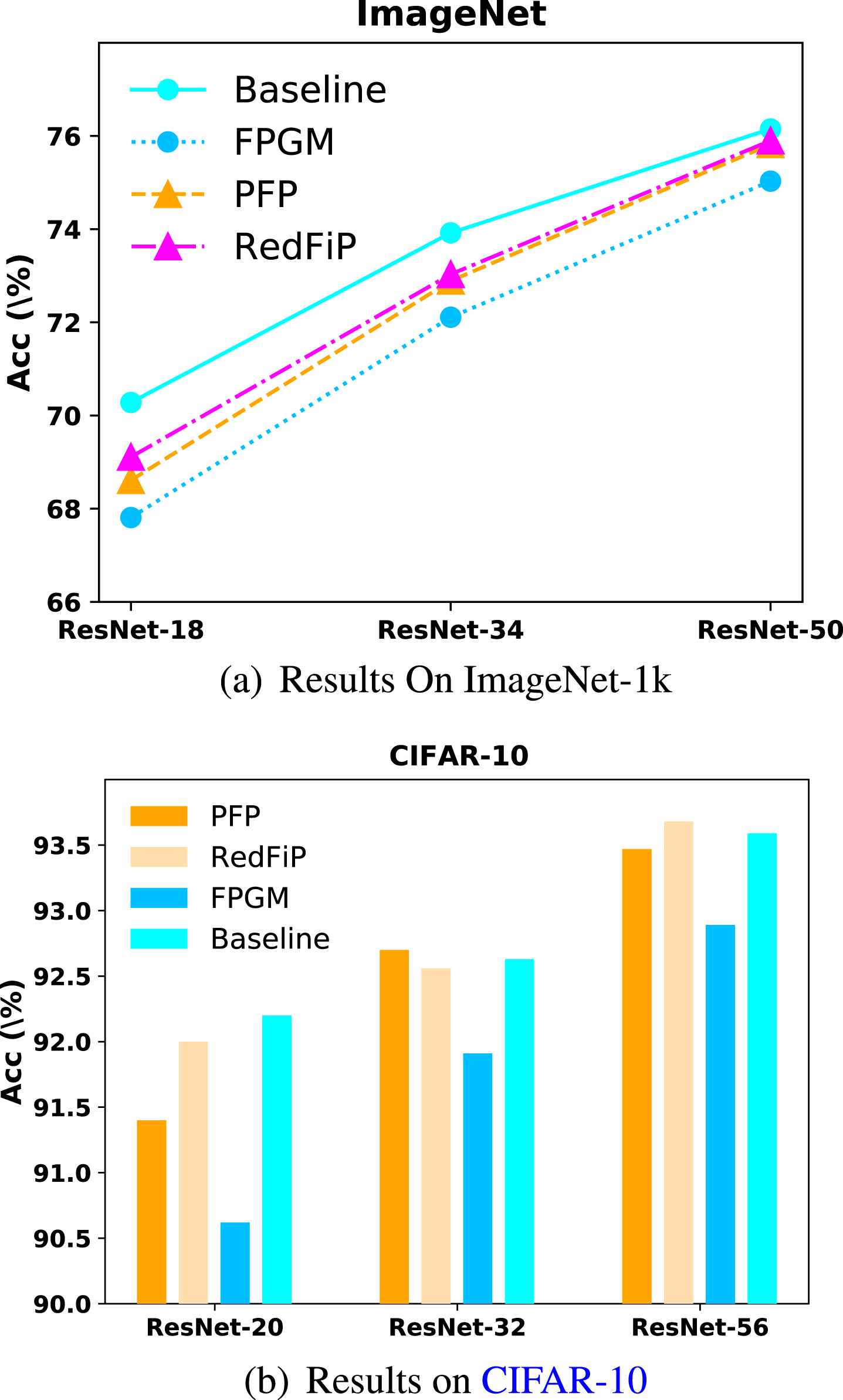This amounts to deactivating the units of filters [?], i.e., they become redundant since zero-valued neurons contribute little to the final decision/inference.

Fig. 1

The results of the proposed pruning strategies, RedFiP and PFP on ImageNet-1k and CIFAR-10. (a) On ImageNet, PFP outperforms the state-of-the-art FPGM [9] by about 0.8% without finetune. (b) On CIFAR-10, RedFiP and PFP even outperform the baseline for ResNet-32. The figure is best viewed in electronic form.

Seeing much redundancy in very deep CNNs [10], Jonathan [10] proposed that pruning technologies can drastically reduce the total parameters of CNN architectures, making them lighter at the cost of little performance drop. Also, pruning technologies have improved the practicability of deep CNNs as they demand less computational and storage resources. Pruning is becoming an active research direction that can help people explore the importance of components and understand the inference mechanism of CNNs.

The existing pruning methods can be divided into three categories. The first category adds regularization terms in loss functions to reduce the dimensionality of network parameter spaces. The second category adopts Network Architecture Search (NAS) for getting the appropriate pruned architectures, to find the most compact models by reinforcement learning and greedy algorithms. The third category directly prunes components and filters of CNNs according to the criteria measuring the their importance. These three categories will be introduced in Section 2.

This paper focuses on the structured component pruning methods because the pruned components can be readily dropped instead of zero-valued setting of the redundant neurons in many unstructured pruning methods. This means that the structured methods can be used in practical applications. Also, the study on structured component pruning technologies helps understand the inherent logic of deep convolutional neural networks.

However, as stated in Section 2.3, one drawback of the structured component pruning method is that the designed criteria treat the filters in different layers equally. They implicitly assume that all filters or layers have an identical importance (contribution) to the whole architecture. However, different layers actually are responsible for extracting different abstract levels of information, and thus the redundancy degree may also differ from one layer to another. Observing this, we aim to develop a pruning scheme that reduces a varying number of filters at each layer according to its redundancy.

To more effectively suppress the redundant kernels at different layers, we firstly analyze the redundancy degree of each layer, and then propose the Redundancy-dependent Filter Pruning (RedFiP) strategy according to the redundancy of each layer. Our analysis shows that the redundancy degree of the shallow layers is significantly lower than middle and deep layers, and hence the shallow layers are more improper to be pruned. The shallow layers are typically responsible for extracting low-level features such as edge, contour, and gradients, etc., and various low-level features are important for deeper layers to generate certain abstract features for specific tasks. As shown in Fig. 1(a), RedFiP outperforms the SOTA pruning strategy, FPGM, by a lot.

According to the redundancy analysis and experimental results shown in Section 3, we observe that filters in deep layer are more suitable for being pruning than those in shallow layers. Seeing this, we further present the Phased Filter Pruning (PFP) strategy to simplify the implementation of RedFiP. PFP divides all layers into three phases, and the layers within each phase share the same pruning rate instead of the original layer-wise pruning rate.

In addition to the implementation simplicity, another advantage of PFP is that deep layers generally contain much more filters and filter channels than shallow layers, and hence a larger pruning proportion in deep layers reduces more parameters of the whole model. For examples, for ResNet20 with three phases (16, 32, and 64-channel kernel per phase), phase 1 (layer 1 ∼ layer 7) and phase 3 (layer 14 ∼ layer 19) contain 5.25% and 75.8% parameters of the whole model. Therefore, PFP can prune more parameters than the existing methods while maintaining the performance of pruned networks. PFP can be readily applied to any architectures, especially the architectures containing a larger number of layers. The highlight results of PFP are also shown in Fig. 1(b).

It is worth mentioning that, when the smallest-norm criterion is used to prune filters, unlike [11], RedFiP explores the effect of pruning different proportion filters in different layers during training stage (i.e., soft pruning proposed in [12]) instead of after training (i.e., hard pruning). Also, [11] pruned both the m filters of the smallest norms and their corresponding output feature maps, i.e., they will not be used by the kernels in next layer. Unlike [11], RedFiP preserves these feature maps and still uses them in the convolution process in next layer. This means RedFiP prunes the filters in different layers independently, which is simpler than [11]. In addition, this work employs the largest-similarity criterion together with the smallest-norm criterion [9]. Only the smallest-norm criterion may prune the filters of smaller norms but important for the whole structure, leading to notable performance decrease in some cases.

The contributions of our proposed strategies are summarized as follows.

The redundancy of a layer is defined that encodes how much fraction of each layer can be pruned. Then Redundancy-dependent Filter Pruning (RedFiP) strategy is proposed that prunes filters by a varying fraction depending on their redundancy. Experiment results show that RedFiP outperforms the smallest-norm [11, 12], largest-similarity and their combined criteria (used in [9]), which treat equally all kernels of different layers.

A simpler phase-wise pruning strategy, Phased Filter Pruning (PFP), is proposed that divides layers into three phases and the layers within each phase share the same pruning rate. The PFP is much easier to be applied to the existing architectures such as ResNet and still outperforms the state-of-the-art strategies by a large margin.

The redundancy analysis and experimental results show that there are more redundant kernels in deep layers than in shallow layers. It indicates that a sufficiently large number of various kernels in charge of extracting low-level image features play an indispensable role for generating high-level semantic information.

2 Related Works

2.1 Regularization

Many researchers focus on designing different regularizations to reduce the dimensionality of network parameter space. Han et al. [13] simply added L₁ and L₂ norm of all parameters in loss function to get more parameters close to zero. Louizos et al. [14] proposed L₀ regularization to reduce the parameters and learn a sparse neural network. L₀ regularization term encourages the weights of some filters to be exactly zero. Alvarez et al. [15] designed a regularization item to learn the number of neurons. A group of sparsity regularizations on the parameters were used to make the overcomplete network more compact and sparse by sufficiently employing structured sparsity.

2.2 NAS-based strategies

In 2018, AMC [16] was proposed to use the learning-based pruning policy by NAS instead of the conventional rule-based policy. Following [16], many NAS-based methods were proposed. Yu et al. [17] proposed a simple and one-shot method, named AutoSlim, to get better performance under the fixed constrained resources (e.g., FLOPs, model size, etc.). Instead of training a lot of architectures for finding the the best architecture by reinforcement learning, a simple slimmed architecture is trained to achieve network accuracy of different channel configurations. Dong et al. [18] proposed TAS applying a differentiable NAS method to search directly for a network with flexible channel and layer sizes to break the architecture limitation. Furthermore, Wang et al. [19] proved that a pre-trained model is not necessary and a fully-trained over-parameterized model will reduce the search space for the pruned structure. Furthermore, Meta-Learning is also applied for model pruning. Liu et al. [20] proposed a method based on Meta-Learning to generate the weights of pruned networks.

2.3 Component Pruning strategies

The key of component pruning is to measure the importance of the pruned components. Many criteria measuring the importance of network components were proposed. Hertz et al. [21] proposed a weight importance measuring criterion according to the magnitude of the weights. Variant magnitude measures were subsequently proposed, e.g., the weights and filters are pruned according to their L₂ or L₁ norm [11, 12].

Hassibi et al. [22] proposed a strategy that measures the importance of each weight by its second order derivative. Joseph et al. [8] used the gradient norm [23] to measure the importance of each filter and evaluated the impact of a filter on error. He et al. [24] proposed an iterative two-step algorithm to select pruned channels based on LASSO regression. He et al. [9] proved that the criteria only measuring the norm are not suitable for all situation. They proposed a novel largest-similarity criterion to measure whether a filter is ‘replaceable’ or not, instead of measuring the usefulness of the filters only according to the norm.

Besides the importance of filters, Wang et al. proposed that identifying structural redundancy plays a more essential role than importance measuring. [25] verified that pruning in the layer(s) with the most structural redundancy outperforms pruning the least important filters across all layers. Moreover, He et al. proposed LFPC [26] to learn the filter pruning criteria for replacing the handmade criteria and achieving adaptive pruning criteria. Gao et al. proposed a performance prediction network [27] to directly guide the channel pruning via the pruned sub-network performance.

Recently, dynamic channel pruning technology [28] becomes more and more popular. The structural pruned channels should be dependent on the input samples. Liu et al. proposed a novel method [29], which focuses on the difference between sample, to learn the instance-wise sparsity adaptively. The informative features for different instances are identified. Furthermore, Tang et al. proposed ManiDP [30] to remove redundant filters by aligning the recognition complexity and feature similarity between images.

3 Method

This section represents the proposed RedFiP and PFP strategies for effectively pruning filters at each layer. Contrary to the general understanding of filter redundancy, we will show that the deep layers have higher redundancy degree. We firstly define redundancy of norm and similarity. Then the definition will be used to analyze the layer-wise and phase-wise redundancy pattern across the whole networks. The common stacked convolutional neural networks and ResNets [1] are used in our analyses. According to the redundancy pattern, RedFiP and PFP are proposed. These two strategies are visualized in Fig. 2.

Fig. 2

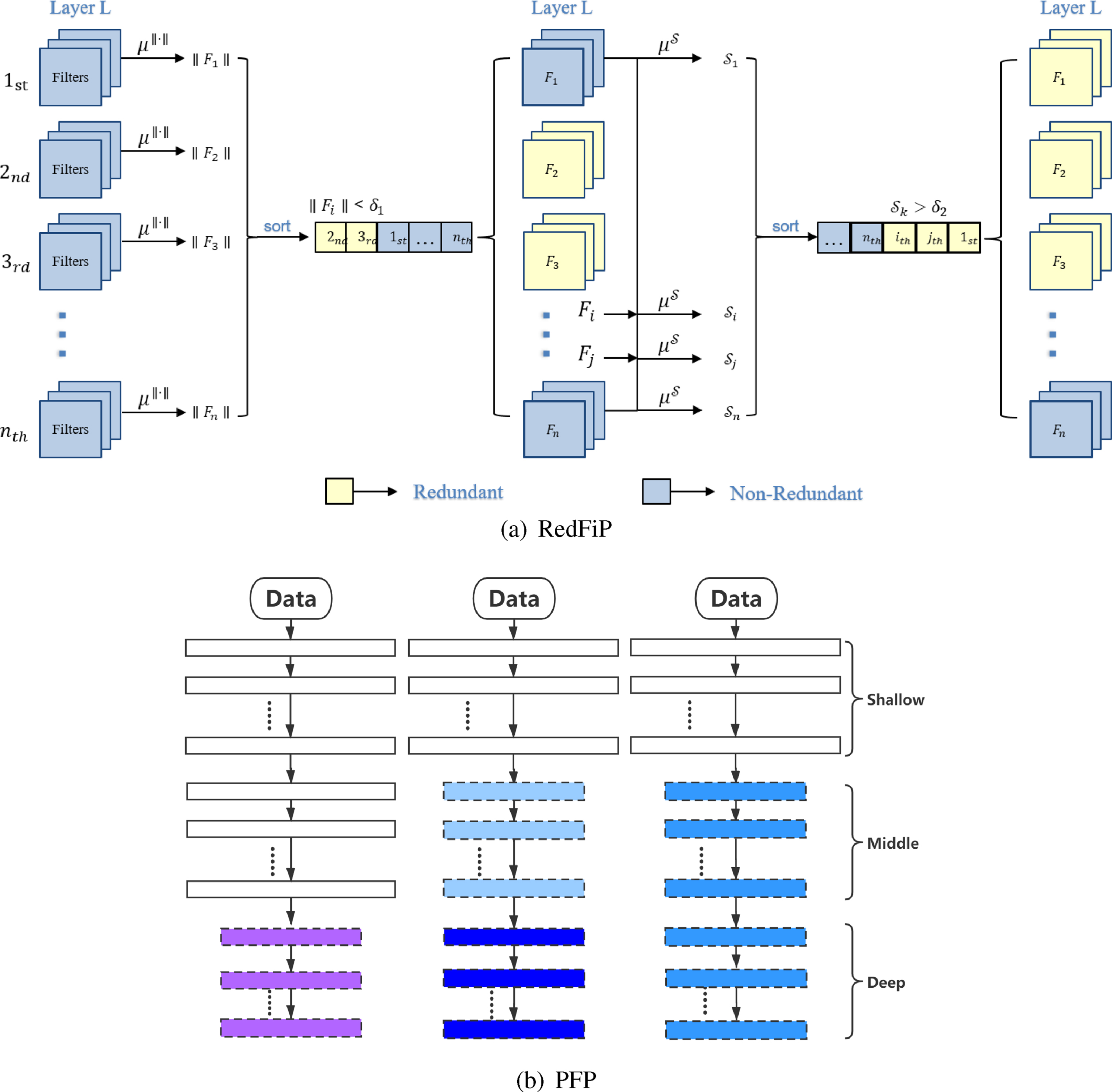
The filter redundancy and the proposed strategies. (a) RedFiP strategy. For each layer, the redundancy degree is computed based on the norm and similarity of filters, and the pruning rate is determined by the layer-wise redundancy. (b) PFP strategy, the layers are divided into three phases and the filters within a phase share the same pruning rate. The larger the pruning rate is, the darker the color of this phase is.

3.1 Redundancy definition

Let N_L denote the number of convolutional layers, and L_i (0 ≤ i ≤ N_L - 1) represents the i_th layer. To define the redundancy of the L_i layer, we firstly define the redundancy of each filter F_i,j in L_i, where 0 ≤ j ≤ N_i - 1 and N_i is the filter number of L_i. A step function is to encode the filter-wise redundancy of target networks to analyze the redundancy pattern across the whole networks. The responding value δ of the step function is determined by the target parameter pruning (such as 30% parameters of the whole network) or the value of acceptable performance drop. These two values are preset by the pruning tasks.

The norm redundancy of F_i,j is defined as $R_{i, j}^{∥ \cdot ∥} = {\begin{matrix} 1, & ∥ F_{i, j} ∥ < δ_{1} \\ 0, & ∥ F_{i, j} ∥ \geq δ_{1} \end{matrix},$ (1) where ∥F_i,j∥ denotes the norm of F_i,j averaged across the channel dimensionality. Similarly, the similarity redundancy is defined as

$R_{i, j}^{S} = {\begin{matrix} 1, & S (F_{i, j}) > δ_{2} \\ 0, & S (F_{i, j}) \leq δ_{2} \end{matrix},$ (2) where $S (F_{i, j})$ is the average similarity between F_i,j and all other filters F_i,p ∈ L_i, p = 0, …, N_i - 1, p ≠ j. Here, the similarity between the two filters F_i,j and F_i,p is defined to be inversely proportional to their Euclidean distance. Formally,

$S (F_{i, j}) = ((\sum_{p = 0}^{N_{i} - 1} d (F_{i, j}, F_{i, p})) / N_{i})^{- 1},$ where K is the kernel size of F_i,j and C is the channel number of F_i,j.

Finally, the redundancy of the whole architecture is defined as the summation of the redundancy of every filter over all layers, formally $Red = \sum_{i = 0}^{N_{L} - 1} \sum_{j = 0}^{N_{i} - 1} (R_{i, j}^{∥ \cdot ∥} + R_{i, j}^{S}) .$ (3)

The redundancy degree defined in Equation (3) can represent that of three pruning criteria: norm criterion, similarity criterion, and their combined criterion. In Equation (1) and (2), except pruning task requests, δ₁ and δ₂ are also experimentally determined to find a good trade-off between smallest-norm and largest-similarity criteria. This is still an open question in [9], which proposed largest-similarity criterion and used it combined with smallest-norm criterion to get a better performance. δ₁ and δ₂ typically take the value in ranges [0.5, 0.7] and [0.9, 1] for ResNet-20 on CIFAR-10 respectively, and more details can be seen in Section 4.1. It is worth mentioning that the proper values for the two thresholds δ₁ and δ₂ change with the architecture of networks, the training datasets. In general, the larger the architecture, the larger the δ₁ and the smaller the δ₂, meaning a looser condition for defining a filter to be redundant in Equation (1) and (2).

3.2 RedFiP strategy

This section will analyze the redundancy degree of filters and then prune the filters according to the redundancy. Since the redundancy of each layer may differ from another, one straightforward layer-wise strategy is to prune a proportion of filters at each layer according to the defined redundancy degree. Alternatively, a simpler strategy that is much easier to be implemented in existing architectures will be discussed in Section 2.3.

To see how much the redundancy exists, we build a generic CNN architecture of 20 layers composing of only convolutional layers, BatchNorm layers, and ReLU layers. We firstly analyze the norm redundancy of each layer when δ₁ in Equation (1) is set to 1. For the norm redundancy of the first 8 layers, 17 filters are determined to be redundant, while 77 filters are non-redundant. The norm redundancy rate is 18.1%. The middle 6 layers have the norm redundancy 81, and the norm redundancy rate is 48.8%. As a comparison, the deep 6 layers have the norm redundancy 384, and the norm redundancy rate is 100%. Similarly, when δ₁ is 0.8, the norm redundancy rate of shallow layers is 10.6%, while that of deep layers is 100%. When δ₁ is 0.5, the norm redundancy rate of shallow layers is 10.6%, while that of deep layers is 97.4%. The norm redundancy patterns are visualized in Fig. 3(a) and Fig. 3(b).

Fig. 3

The pattern of filter norm and similarity in a 20-layer convolutional neural network. In the norm pattern analyses (a, b, c), The blue bar represents the number of filters with their norms smaller than the threshold δ₁, which means the number of filters can be pruned in this layer under the threshold δ₁. And the pink bar represents the number of filters with their norms larger than δ₁. In the similarity pattern analyses (d, e, f), The blue bar represents the number of filters with their similarities larger than the threshold δ₂, which means the number of filters can be pruned in this layer under the threshold δ₁. And the pink bar represents the number of filters with their similarities smaller than δ₂. (a), δ₁ is set to 1.0; (b), δ₁ is set to 0.8; and (c), δ₁ is set to 0.5; (d), δ₂ is set to 1.3; (e), δ₂ is set to 1.0; (f), δ₂ is set to 0.8.

In some deep layers, the redundancy rate of certain layers may be as high as 100%. However, we cannot prune all filters of these layers convolutional neural networks. For such cases, we firstly select an appropriate threshold for the step function of previous layers, and prune a small proportion of shallow filters, e.g., 5%. For the norm criterion, the redundancy rate for the deep layers will become smaller than 90% [10] by decreasing the threshold of the step function. For examples, if the task requests 40% parameters of the generic CNN being pruned, the previous 13 layers prune 5% parameters of total model. Then the threshold has been reduced to make the redundancy of last six convolutional layers comprise the rest 35% of total parameters. For the similarity criterion, a similar result can be achieved by appropriately increasing the threshold δ₂ in Equation (2). 90% is also a threshold for similarity redundancy rate for each layer.

Then, we continued to analyze the similarity redundancy defined in Equation (2). When δ₂ is 1.3, the similarity redundancy rate of shallow layers is just 15.6%, while that of deep layers is 100%. When δ₂ is 1, similarity redundancy rate of shallow layers is 6.25%, while that of deep layers remains to be 100%. When δ₂ is 0.8, similarity redundancy rate of shallow layers is 0%, while that of deep layers is 100%. The similarity redundancy patterns are visualized in Fig. 3(c) and 3(d). The norm and similarity redundancy indicate that the deep layers have a much higher redundancy rate than shallow layers and so a higher proportion of filters can be pruned at deep layers.

To further verify the effectiveness of the defined norm and similarity redundancy, we conduct another kind similar analysis on ResNet-20 [1]. Fig. 4 shows the norm and similarity redundancy. Again, it can be observed that deeper layers contain much more redundancy than shallower layers. In fact, the redundancy results observed in our experiments are in accordance with what are reported in [31] that shows shallow layers usually need more filters to represent various features whereas deep layers need much fewer filters to represent the highly abstract semantic information. One possible explanation for these results is that deeper layers are gradually focused on the extraction of the semantic information about objects in an image as well as their location [32, 33]. This hence means that the non-object regions will require much fewer deep-layer filters.

Fig. 4

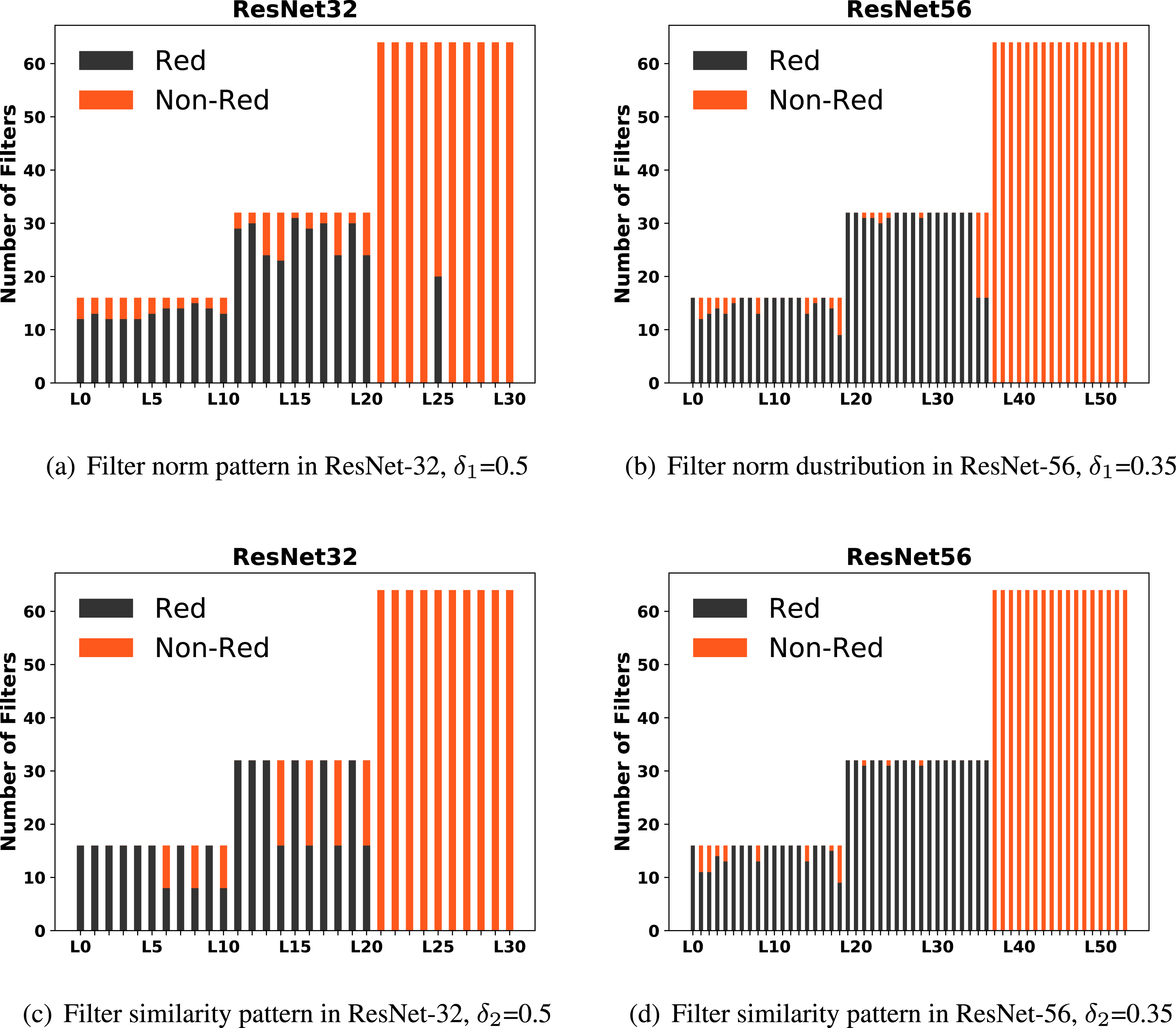
The pattern of filter norm and similarity in ResNets. The blue bar represents the number of filters with their norms / similarities smaller / larger than the threshold δ₁ / δ₂. The pink bar represents the number of filters with their norms / similarities larger / smaller than δ₁ / δ₂.

With the defined norm and similarity redundancy, this work presents a redundancy dependent pruning strategy, RedFiP, that prunes filters according to the calculated redundancy degree at each layer. RedFiP is shown in Fig. 2(a). The advantage of this strategy lies in that it is tailored for each layer and thus the layer-wise redundant filters will be pruned to the maximum degree under the requests of tasks.

3.3 PFP strategy

Despite its advantages, RedFiP is relatively difficult to be implemented since the hyperparameters δ₁ and δ₂ in Equations (1) and (2) need to be finely tuned for individual networks and datasets. Also, δ₁ and δ₂ are carefully determined to ensure that not all filters in one layer are pruned, like the careful strategy described in Section 3.2. This can be quite cumbersome and require specific tuning skills. To facilitate the implementation, this work further proposed an alternative pruning strategy, Phased Filter Pruning (PFP), that divides all layers into three phases: shallow phase, middle phase, and deep phase for phase-wise pruning. Layers in the same phase share the same pruning rate in phase-wise strategy.

According to the redundancy degree calculated in Section 3.1, shallow layers responsible for extracting various low-level features can hardly be pruned. Middle layers conveying shallow features to the high-level semantic information have a little redundancy and can be partly pruned. Compared with shallow and middle layers, deep layers have a much higher redundancy degree and can be substantially pruned while the performance drops little.

The shallow phase contains fewer and more important filters than those in middle and deep phases according to the analysis in Section 3.2. PFP maintains all filters in shallow phase, while pruning severely filters in middle and deep phases. Each phase shares the same pruning rate instead of layer-wise determined strategy, RedFiP. As the example in Section 3.2, if only 50% filters in deep phase are pruned, the reduced parameters would comprise 32.9% of total model parameters. PFP is a phase-wise strategy and much simpler in the threshold selection aspect than the layer-wise RedFiP.

We evaluate the PFP strategy by designing three schemes shown in Fig. 2(b). The first scheme is to only prune the filters of the deep phase, as shown in the left column in Fig. 2(b). The second scheme is to prune the filters of the middle and deep phases by the same proportion. are pruned, as shown in the middle column in Fig. 2(b). The third scheme is also to prune the filters of the middle and deep phases, but the deep phase has a higher pruning proportion, as shown in the right column of Fig. 2(b).

In addition, another phenomenon is observed. The last layer’s high similarity may actively maintain the invariance of classification to improve the confidence of the right decision. This maybe provide another view of the reason why the ReLU neural network always produces the confidence so high [34].

4 Experiments

In this section, the proposed RedFiP and PFP strategies are compared with the norm-based strategies SFP [12] and MIL [35]. Also the similarity-based strategy FPGM [9] is used. The experiments are evaluated on datasets CIFAR-10, CIFAR-100, and ImageNet-1k [36]. We directly use the reported results of SFP, MIL, and FPGM in [9 , 35] except the results of FPGM on CIFAR-100, which was not reported in [9]. To make the experimental comparison more complete, we evaluated the FPGM on CIFAR-100 with the code provided by [9]. The implementation of RedFiP and PFP are based on the source code of FPGM.

ResNet-20, ResNet-32, and ResNet-56 are adopted to serve as the baseline. ResNet-110 is not used since a large number of layers contain too many redundant filters for training on the small datasets CIFAR-10 and CIFAR-100.

ResNets are divided into 3 phases, and each phase contains (depth - 2) / 3 convolutional layers. The hyperparameters of all ResNets are similar to those of FPGM [9]. For PFP, Table 1 summarizes the three schemes devised to prune the filters of phase 2 and/or 3.

Table 1
Description of different schemes for the PFP strategy

Scheme Description

PFP-S₃ Only filters in phase 3 are pruned.

PFP-S_2∼3 Filters in phase 2 and phase 3 are pruned by the same proportion.

PFP-S_2≺3 Filters in phase 2 and phase 3 are pruned but by different proportions.

Scheme	Description
PFP-S₃	Only filters in phase 3 are pruned.
PFP-S_2∼3	Filters in phase 2 and phase 3 are pruned by the same proportion.
PFP-S_2≺3	Filters in phase 2 and phase 3 are pruned but by different proportions.

Inspired by the work [37], we train the networks from scratch and apply the soft filter pruning. SGD is used to optimize the training model and the initial learning rate is set to 0.01. The learning rate is divided by 5 when the training epoch equals 60, 120, and 150. Additionally, the warmed up [38] strategy is used. Decay is set to 0.0005 to make the network robust against noise.

For each experiment, we repeated 5 times to alleviate the effect of random initialization, and the 5-time average test accuracy is reported. The proposed RedFiP strategy is compared with FPGM and SFP, and the results are listed in Table 2. The results of the proposed PFP are listed in Table 4. To show the universality of RedFiP and PFP, we also apply them to VGG. The results on CIFAR-10 are given in Table 6. In Section 4.4, filters in shallow phase are severely pruned for ablation study.

Table 2

Comparison between RedFiP and state-of-the-art strategies for ResNets on CIFAR-10 and CIFAR-100. The pruning strategies are listed in ‘Method’ column, the pruning rates of the total parameters are listed in parentheses. The values listed in ‘Acc ↓’ mean that the test accuracy errors between the pruned networks and the non-pruned networks

Depth	CIFAR-10			CIFAR-100			FLOPs ↓(%)
Method	Pruned acc.	Acc ↓	Method	Pruned acc.	Acc ↓
20	FPGM(30%)	91.09	1.11	FPGM(30%)	65.52	2.68	42.2
	FPGM(40%)	90.62	1.58	FPGM(40%)	64.20	4.00	54.0
	SFP[12](30%)	90.83(±0.31)	1.37	–	–	–	42.2
	RedFiP(22%)	92.23(±0.16)	-0.03	–	–	–	31.0
	RedFiP(38%)	92.00(±0.26)	0.20	RedFiP(36%)	66.03(±0.24)	2.17	51.0
32	FPGM(40%)	91.91	0.72	FPGM(40%)	67.19	3.70	54.0
	MIL[35]	90.74	1.59	FPGM(30%)	67.72	3.17	31.2
	RedFiP(40%)	92.56(±0.27)	0.07	–	–	–	54.0
	RedFiP(36%)	92.74(±0.3)	-0.11	RedFiP(36%)	68.40(±0.24)	2.49	49.0
56	FPGM(40%)	92.89	0.70	FPGM(40%)	69.24(±0.12)	2.92	54.0
	SFP[12](40%)	92.26(±0.31)	1.33	–	–	–	52.6
	RedFiP(40%)	93.68(±0.24)	-0.09	RedFiP(40%)	70.62(±0.23)	1.64	54.0

4.1 Redundancy Dependent Filter Pruning

The combination of smallest-norm and largest-similarity criteria is used in RedFiP evaluation experiments, which is similar to pruning criteria FPGM-Mixed [9]. For simplifying the description, we use the form like RedFiP (30%) to represent that 30% of total parameters are pruning by the strategy RedFiP in the following sections. Table 2 gives the best results of RedFiP (40%), FPGM (40%), and SFP (30%) for ResNets of different layers on CIFAR-10/100. For ResNet-20, the RedFiP outperforms FPGM-Mixed and SFP by 0.91% and 1.17% in terms of the classification accuracy on CIFAR-10. On CIFAR-100, RedFiP (36%) outperforms FPGM-Mixed (30%) by 0.51%. Also, RedFiP (40%) outperforms FPGM-Mixed (40%) by 1.38%.

It is also worth noting that when 22% parameters are pruned by RedFiP, the pruned ResNet-20 achieves the test accuracy 92.23% on CIFAR-10, which is even higher than the non-pruned ResNet-20. This indicates the redundancy existence in the deep neural networks and verifies the benefit of the RedFiP.

Similarly, for ResNet-32 and ResNet-56, RedFiP (40%) achieved 0.68% and 0.79% accuracy improvements on CIFAR-10. Also, on CIFAR-100, 1.21% and 1.28% accuracy improvements are achieved for ResNet-32 and ResNet-56.

4.2 Phased Filter Pruning

This section presents the evaluation performance of the Phased Filter Pruning (PFP) strategy. For the implementation of pruning filters, we apply the smallest-norm and largest-similarity criteria to suppress filters at each phase. Let Rt_i (n % , v %) denote the pruning rates at the i_th phase with the smallest-norm and largest-similarity criteria. (n+ v) % means the total pruning rate in the i_th phase.

4.2.1 Filters in different phases are pruned for Conv-20

To see the redundancy of different phases, we firstly build a simple stacked CNNs of 20 convolutional blocks. Each block contains a convolutional layer, a Batch Normalization (BN) layer, and a ReLU layer. The stacked 20-layer CNN is divided in 4 phases, and each phase contains 6 layers. We picked the 6 layers to be {, [2, 8] , [12, 18] , [14, 20]}. For each experiment, 40% filters of the corresponding phase are pruned by the smallest-norm criterion, and all layers in each phase share the same pruning rate. Table 3 gives the classification accuracies of the pruned models. Obviously, when the 4_th phase is pruned, the pruned model provides the best test accuracy even if it is pruned the most parameters. The simple comparison experiments verify that the deep layers contain more redundancy. Also, the pruned model provides 87.3% classification accuracy, which is higher than the baseline of non-pruned model.

Table 3
Filters in different phases for Conv-20 on CIFAR-10

Layers Non-Prune 0-6 2-8 12-18 14-20

Acc.(%) 86.27 85.53 85.9 87.13 87.3

Layers	Non-Prune	0-6	2-8	12-18	14-20
Acc.(%)	86.27	85.53	85.9	87.13	87.3

Table 4

Comparison between PFP and state-of-the-art strategies for ResNets on CIFAR-10 and CIFAR-100. The pruning strategies are listed in ‘Method’ column, the pruning rates of the total parameters are listed in parentheses. The values listed in ‘Acc ↓’ mean that the test accuracy errors between the pruned networks and the non-pruned networks

Depth	CIFAR-10			CIFAR-100			FLOPs ↓(%)
Method	Pruned acc.	Acc. ↓	Method	Pruned acc.	Acc. ↓
20	FPGM(30%)	91.09	1.11	FPGM(30%)	65.52(±0.24)	2.68	42.2
	SFP[12](30%)	90.83(±0.31)	1.37	PFP-S₃(30%)	65.98(±0.23)	2.22	42.2
	PFP-S₃(30%)	91.76(±0.17)	0.44	PFP-S₃(30%)	65.98(±0.23)	2.22	42.2
	PFP-S_2≺3(30%)	91.51(±0.22)	0.69	PFP-S_2≺3(30%)	65.97(±0.39)	2.23	42.2
20	FPGM(40%)	90.62	1.58	FPGM(40%)	64.20(±0.24)	4.00	54.0
	PFP-S₃(40%)	91.40(±0.22)	0.80	PFP-S₃(40%)	65.07(±0.53)	3.13	54.0
	PFP-S_2∼3(40%)	91.28(±0.45)	0.92	PFP-S_2∼3(40%)	65.02(±0.45)	3.18	54.0
	PFP-S_2≺3(42%)	91.19(±0.2)	1.01	PFP-S_2≺3(42%)	64.80(±0.32)	3.40	55.0
32	FPGM(40%)	91.91	0.72	FPGM(40%)	67.19(±0.24)	3.70	54.0
	MIL[35]	90.74	1.59	–	–	–	31.2
	PFP-S₃(40%)	92.70(±0.14)	-0.07	PFP-S₃(40%)	67.97(±0.25)	2.92	54.0
	PFP-S_2∼3(40%)	92.30(±0.19)	0.33	PFP-S_2∼3(40%)	67.65(±0.6)	3.24	54.0
	PFP-S_2≺3(42%)	92.35(±0.14)	0.28	PFP-S_2≺3(42%)	67.47(±0.14)	3.42	54.0
56	FPGM(40%)	92.89	0.70	FPGM(40%)	69.24(±0.12)	2.92	54.0
	SFP[12](40%)	92.26(±0.31)	1.33	–	–	–	52.6
	PFP-S₃(40%)	93.47(±0.18)	0.12	PFP-S₃(40%)	70.25(±0.31)	1.91	54.0
	PFP-S_2∼3(40%)	93.29(±0.24)	0.30	PFP-S_2∼3(40%)	70.50(±0.28)	1.66	54.0
	PFP-S_2≺3(42%)	93.33(±0.13)	0.26	PFP-S_2≺3(42%)	70.13(±0.18)	2.03	54.0

4.2.2 PFP on CIFAR-10.

The scheme PFP-S₃ only prunes filters in phase 3. In phase 3, 40% filters, which accounts for 30% of the total network, are pruned. Rt₃ (10 % , 30 %) outperforms FPGM-Mixed (30%) by 0.67% for ResNet-20. Then 54% filters in phase 3, which accounts for 40% of the total network, are pruned. As listed in in Table 4, 0.78%, 0.79% and 0.58% improvements are achieved compared with FPGM-Mixed (40%) for ResNet-20, ResNet-32, and ResNet-56 respectively. Especially, the result of PFP-S₃ (40%) outperforms FPGM-Mixed (30%) by 0.31% for ResNet-20.

The scheme PFP-S_2∼3 prunes filters in phase 2 and 3 with the same rate, without pruning phase 1. Table 4 lists the results. Rt_2,3 (20 % , 24 %), pruning 40% of total network parameters, outperforms FPGM-Mixed (40%) by 0.66% for ResNet-20. Similar pruning schemes achieve 0.39% and 0.40% improvements for ResNet-32 and ResNet-56 respectively.

For evaluating PFP-S_2≺3 listed in Table 1, we use Rt₂ (10 % , 10 %)-Rt₃ (20 % , 30 %) to denote that 10% parameters are pruned with both the smallest-norm and largest-similarity criteria at phase 2, while 20% parameters are pruned with smallest-norm criterion and 30% with largest-similarity criterion at phase 3. This scheme prunes about 42% parameters of the whole network, which is higher than the 38% of PFP-S_2∼3. It outperforms FPGM-Mixed (40%) by 0.57%, 0.44%, and 0.44% for ResNet-20, ResNet-32, and ResNet-56, respectively. The Rt₂ (10 % , 10 %)-Rt₃ (15 % , 20 %) scheme prunes about 30% parameters of the whole network, and outperforms FPGM-Mixed (30%) by 0.42% for ResNet-20.

The results on CIFAR-10 listed in Table 4 clearly show that the PFP-pruned networks have a comparable feature representation ability to the non-pruned network. Compared with FPGM, PFP can prune a higher rate of filters while achieving better performance. Also, PFP-S₃ performs better than PFP-S_2≺3, and PFP-S_2≺3 outperforms PFP-S_2∼3. This verifies that the filters in deeper layers are more suitable for being pruned.

4.2.3 PFP on CIFAR-100.

Like Section 4.2.2, we continue to evaluate the three schemes of PFP on CIFAR-100. PFP-S₃ (30%) prunes the parameters of ResNet-20 and evaluated on CIFAR-100. As is listed in Table 4, it achieves 0.46% accuracy improvement over FPGM-Mixed (30%). Similarly, PFP-S₃ (40%) outperforms FPGM-Mixed (40%) by 0.87%. For ResNet-32 and ResNet-56, PFP-S₃ (40%) also outperforms FPGM-Mixed (40%) by 0.78% and 1.01% respectively.

For PFP-S_2∼3, Rt_2,3 (10 % , 34 %) scheme is used to prune 40% parameters of total parameters. It outperforms FPGM-Mixed (40%) by 0.78%, 0.46%, and 1.26% for ResNet-20, ResNet-32, and ResNet-56 respectively. For the scheme PFP-S_2≺3, Rt₂ (10 % , 10 %)-Rt₃ (15 % , 20 %) scheme is used to prune 30% parameters. It outperforms FPGM-Mixed (30%) by 0.45% for ResNet-20. Similarly, PFP-S_2≺3 (42%) outperforms FPGM-Mixed (40%) by 0.6%, 0.28%, and 0.89% for ResNet-20, ResNet-32, and ResNet-56 respectively.

Similar to the evaluation on CIFAR-10, PFP-S₃ achieves the highest accuracy on CIFAR-100, and outperforms FPGM by a large margin. Also, PFP-S₃ is slightly inferior to RedFiP on CIFAR-100, which again tells that the deeper layers have more redundancy and the much simpler scheme PFP-S₃ can effectively prune the network without fine-tuning the hyperparameters.

4.2.4 PFP and RedFiP on ImageNet-1k

For experiments on ImageNet-1k, the initial output-channel number is 64, and the maximum output-channel number is 512, like a typical ResNet architecture for ImageNet-1k.

On ImageNet-1k, PFP is applied to three architectures, ResNet-18, ResNet-34, and ResNet-50, to investigate its performance. Also, we investigate the performance of the PFP-pruned structures with finetuning. For RedFiP, it is applied to the three architectures, but finetuning is not used as its performance without finetuning is already comparable to that of PFP with finetuning. Among the three schemes of PFP, PFP-S₃ achieves the best test classification accuracy for all the three structures, and os only the results of PFP-S₃ are reported.

All evaluated results on ImageNet-1k are reported in Table 5. For ResNet-18, ResNet-34, and ResNet-50 without finetuning, PFP-S₃ (30%) outperforms FPGM (30%) by 0.8%, 0.78%, and 0.79%. While all pruned models are fine tuned, PFP-S₃ (30%) outperforms FPGM (30%) with finetuning by 0.59%, 0.84%, and 0.5% for ResNet-18, ResNet-34, and ResNet-50. RedFiP (30%) outperforms FPGM (30%) by 1.3%, 0.92%, and 0.87% for these three architectures on ImageNet-1k.

Table 5
Experimental results comparison between our strategies and state-of-the-art strategies on ImageNet for ResNets. The experiments with and without finetuning are conducted. For ImageNet-1k, only 30% parameters are pruned and the best test accuracies are in bold

Depth Method Fine- Baseline Pruned Top-1 Baseline Pruned Top-5 FLOP↓(%)

(top-1 %) acc. (top-1 %) Acc ↓ (top-5 %) acc. (top-5 %) Acc ↓

18 MIL[35] × 69.98 66.33 3.65 89.24 86.24 2.30 34.6

SFP[12] × 70.28 67.10 2.50 89.63 87.78 1.63 41.8

FPGM(30%) × 70.28 67.81 2.47 89.63 88.11 1.52 41.8

RedFiP(30%) × 70.28 69.11 1.17 89.63 89.37 0.26 40.6

PFP-S₃(30%) × 70.28 68.61 1.67 89.63 89.13 0.5 41.8

FPGM(30%) ✔ 70.28 68.41 1.87 89.63 88.48 1.15 41.8

PFP-S₃(30%) ✔ 70.28 69.02 1.26 89.63 89.37 0.26 41.8

SFP[12] × 73.92 71.83 2.09 91.62 90.33 1.29 41.1

34 FPGM(30%) × 73.92 72.11 1.81 91.62 90.69 0.93 41.1

RedFiP(30%) × 73.92 73.03 0.89 91.62 91.19 0.43 40.2

PFP-S₃(30%) × 73.92 72.89 1.03 91.62 90.91 0.71 41.1

PFEC[11] ✔ 73.23 72.17 1.06 – – – 24.2

FPGM(30%) ✔ 73.92 72.63 1.29 91.62 91.08 0.54 41.1

PFP-S₃(30%) ✔ 73.92 73.47 0.45 91.62 73.47 0.11 41.1

50 SFP[12] × 76.15 74.61 1.54 92.87 92.06 0.81 41.8

FPGM(30%) × 76.15 75.03 1.12 92.87 92.40 0.47 42.2

RedFiP(30%) × 76.15 75.90 0.25 92.87 93.01 -0.14 43.1

PFP-S₃(30%) × 76.15 75.82 0.33 92.87 92.89 -0.02 43.8

SFP[12] ✔ 76.15 62.14 14.01 92.87 84.60 8.27 41.8

CP[24] ✔ – – – 92.20 90.80 1.40 50.0

FPGM(30%) ✔ 76.15 75.59 0.56 92.87 92.63 0.24 42.2

PFP-S₃(30%) ✔ 76.15 76.09 0.06 92.87 93.02 -0.15 43.8

Depth	Method	Fine-	Baseline	Pruned	Top-1	Baseline	Pruned	Top-5	FLOP↓(%)
18	MIL[35]	×	69.98	66.33	3.65	89.24	86.24	2.30	34.6
	SFP[12]	×	70.28	67.10	2.50	89.63	87.78	1.63	41.8
	FPGM(30%)	×	70.28	67.81	2.47	89.63	88.11	1.52	41.8
	RedFiP(30%)	×	70.28	69.11	1.17	89.63	89.37	0.26	40.6
	PFP-S₃(30%)	×	70.28	68.61	1.67	89.63	89.13	0.5	41.8
	FPGM(30%)	✔	70.28	68.41	1.87	89.63	88.48	1.15	41.8
	PFP-S₃(30%)	✔	70.28	69.02	1.26	89.63	89.37	0.26	41.8
	SFP[12]	×	73.92	71.83	2.09	91.62	90.33	1.29	41.1
34	FPGM(30%)	×	73.92	72.11	1.81	91.62	90.69	0.93	41.1
	RedFiP(30%)	×	73.92	73.03	0.89	91.62	91.19	0.43	40.2
	PFP-S₃(30%)	×	73.92	72.89	1.03	91.62	90.91	0.71	41.1
	PFEC[11]	✔	73.23	72.17	1.06	–	–	–	24.2
	FPGM(30%)	✔	73.92	72.63	1.29	91.62	91.08	0.54	41.1
	PFP-S₃(30%)	✔	73.92	73.47	0.45	91.62	73.47	0.11	41.1
50	SFP[12]	×	76.15	74.61	1.54	92.87	92.06	0.81	41.8
	FPGM(30%)	×	76.15	75.03	1.12	92.87	92.40	0.47	42.2
	RedFiP(30%)	×	76.15	75.90	0.25	92.87	93.01	-0.14	43.1
	PFP-S₃(30%)	×	76.15	75.82	0.33	92.87	92.89	-0.02	43.8
	SFP[12]	✔	76.15	62.14	14.01	92.87	84.60	8.27	41.8
	CP[24]	✔	–	–	–	92.20	90.80	1.40	50.0
	FPGM(30%)	✔	76.15	75.59	0.56	92.87	92.63	0.24	42.2
	PFP-S₃(30%)	✔	76.15	76.09	0.06	92.87	93.02	-0.15	43.8

Table 6

Pruning scratch VGGNet on CIFAR-10

Method	Baseline	Pruned acc	Acc. ↓
PFEC	93.58	93.31	0.27
FPGM	93.58	93.54	0.04
RedFiP	93.58	93.83(±0.05)	-0.25
PFP	93.58	93.73(±0.13)	-0.15

4.3 VGG on CIFAR-10

Similarly, VGGNet is pruned by RedFiP and PFP on CIFAR-10. Same as the previous experiments, pre-trained model is not used, and each model is trained from scratch. Not surprisingly, these two proposed strategies outperform state-of-the-art strategies and even the baseline. The proposed RedFiP achieves the test classification accuracy 93.83% on CIFAR-10, which outperforms PFEC and FPGM by 0.52% and 0.29% respectively. Also, FPF-S₃ achieves accuracy improvements 0.42% and 0.19% over PFEC and FPGM respectively with the same proportion parameters pruned. RedFiP and PFP also outperform the baseline accuracy by 0.25 and 0.15. For the architecture like VGGNet, good performance is also achieved, and it verifies the effectiveness and universality of our proposed strategies.

4.4 Ablation Experiments

For ablation study, we evaluated the pruning classification performance on CIFAR-10 and CIFAR-100 in the ablation experiments that only shallow layers are pruned by a large pruning rate. As is shown in Fig. 5, when the pruned 40% parameters of the whole model are composed of the filters in the previous layers, especially the filters in shallow phase, the classification performance of ResNet20 drops by 4.4% and 5.66% on CIFAR-10 and CIFAR-100 respectively. When 40% parameters of the shallow layers are pruned, which account for about only 2% parameters of the whole model, the classification performance just slightly outperforms FPGM-Mixed (40%). Seeing this, the performance drop of FPGM-Mixed can be mainly due to the pruned filters in shallow phase. Also, compared with PFP-S₃ (40%), the classification performance of the shallow-layer-pruned model drops by 0.6% and 0.76% on CIFAR-10 and CIFAR-100, indicating the indispensable role of shallow layers in extracting semantic features.

Fig. 5

Shallow layers pruning. Four compared experiments are conducted and the percentages on each bar represents the pruning rate of the whole model. On X-axis, for example, ‘CIFAR-10-20’ represents that ResNet20 is used to evaluate the pruning performance on CIFAR-10. For the legend, ‘Shallow-All’ denotes that we severely pruned filters in previous layers, i.e., shallow, middle phases, and few previous layers in deep phase, for pruning 40% of the whole model. A few previous layers in deep phase are used to be pruned because all parameters of shallow and middle phases only account for 25.2% of total parameters. And ‘Shallow-Less’ represents that only 40% parameters of shallow phase are pruned, and the pruned parameters account for 2% of the whole model.

5 Conclusions

This paper focuses on the problem that filter redundancy differs from layer to layer. Different from the previous pruning strategies, which treat the all layers equally, this paper proposes that different layers should be treated differently according to the redundancy degrees of different layers. Firstly, the redundancy degree is defined based on norm and similarity criteria. The defined redundancy degree is used to analyze the neural networks, and the analysis shows that the redundancy differs from layer to layer. Moreover, the deeper layers have a higher redundancy degree. According to the analysis, a layer-wise pruning strategy RedFiP is proposed. Then a simpler and more effective phase-wise strategy FPF without the layer-wise thresholds is further proposed.

When RedFiP is applied to the ResNets, the pruned models outperforms the SOTA pruning methods. It even outperforms the non-pruned model under a certain pruning rate. This justifies the redundancy definition. Furthermore, the PFP strategy is proposed to essentially simplify the implementation process of RedFiP, and can be readily applied to existing architectures. PFP significantly reduced the parameters while maintaining or even improving the performance, which verifies again the redundancy existence and the value of the proposed pruning strategies.

Footnotes

Acknowledgments

This work was supported by the National Key R&D Program of China under Grant 2019YFF0302601, National Natural Science Foundation of China (No. 62071060), and the Beijing Key Laboratory of Work Safety and Intelligent Monitoring Foundation.

The source code is from ‘https://github.com/he-y/filter-pruning-geometric-median/’

References

, Zhang

, Ren

, et al., Deep residual learning for image recognition. In IEEE Conference on Computer Vision and Pattern Recognition, (2015), pp. 770–778.

Simonyan

and Zisserman

, Very deep convolutional networks for large-scale image recognition. In International Conference on Learning Representations, 2015.

Ioffe

and Szegedy

, Batch normalization: Accelerating deep network training by reducing internal covariate shift. abs/1502.03167, 2015.

Newell

, Yang

and Jia

, Stacked hourglass networks for human pose estimation. In European Conference on Computer Vision, 2016.

Ronneberger

, Fischer

and Brox

, U-net: Convolutional networks for biomedical image segmentation. In International Conference on Medical Image Computing and Computer-Assisted Intervention, 2015.

Huang

, Liu

, Van De Maaten

, et al., Densely connected convolutional networks. In IEEE Conference on Computer Vision and Pattern Recognition, 2017.

Denil

, Shakibi

, Dinh

, et al., Predicting parameters in deep learning. volume abs/1306.0543, 2013.

Paul Cohen

, Lo

Henry Z.

and Ding

, Randomout: Using a convolutional gradient norm to win the filter lottery. In International Conference on Learning Representations, volume abs/1602.05931, 2016.

, Liu

, Wang

, et al., Filter pruning via geometric median for deep convolutional neural networks acceleration. In IEEE Conference on Computer Vision and Pattern Recognition, 2019.

10.

Jonathan

and Michael

, The lottery hypothesis: Finding sparse, trainable neural networks. In International Conference of Learning Representation, 2019.

11.

, Kadav

, Durdanovic

, et al., Pruning filters for efficient convnets. In International Conference of Learning Representation, (2017), volume abs/1608.08710.

12.

, Kang

, Dong

, et al., Soft filter pruning for accelerating deep convolutional neural networks. In International Joint Conference on Artificial Intelligence, (2018), volume abs/1808.06866.

13.

Han

, Pool

, Tran

, et al., Learning both weights and connections for efficient neural networks. In Conference and Workshop on Neural Information Processing Systems, 2015.

14.

Louizos

, Welling

and Kingma

Diederik P.

, Learning sparse neural networks through l0 regularization. In International Conference on Learning Representations, 2018.

15.

Alvarez

Jose M.

and Salzmann

, Learning the number of neurons in deep networks. In Conference and Workshop on Neural Information Processing Systems, 2016.

16.

and Han

, ADC: automated deep compression and acceleration with reinforcement learning. In European Conference on Computer Vision, (2018), volume abs/1802.03494.

17.

and Huang

Thomas S.

, Network slimming by slimmable networks: Towards one-shot architecture search for channel numbers. (2019), CoRR, abs/1903.11728.

18.

Dong

and Yang

, Network pruning via transformable architecture search. (2019), CoRR, abs/1905.09717.

19.

Wang

, Zhang

, Xie

, et al., Pruning from scratch. (2019), CoRR, abs/1909.12579.

20.

Liu

, Mu

, Zhang

, et al., Metapruning: Meta learning for automatic neural network channel pruning. In IEEE International Conference on Computer Vision, 2019.

21.

Hertz

, Krogh

and Palmer

R.G.

, Introduction to the theory of neural computation. 01 2018.

22.

Hassibi

and Stork

David G.

, Second order derivatives for network pruning: Optimal brain surgeon. In Advances in Neural Information Processing Systems, volume 5, (1993), pp. 164–171.

23.

Henry Z.

, Paul Cohen

and Ding

, Prediction gradients for feature extraction and analysis from convolutional neural networks. In IEEE International Conference and Workshops on Automatic Face and Gesture Recognition, 2015.

24.

, Zhang

and Sun

, Channel pruning for accelerating very deep neural networks. In IEEE Conference on Computer Vision, (2017), volume abs/1707.06168.

25.

Wang

, Li

and Wang

, Convolutional neural network pruning with structural redundancy reduction. In Proceedings of the IEEE/CVF Conference on Computer Vision and Pattern Recognition, (2021), pp. 14913–14922.

26.

, Ding

, Liu

, Zhu

, Zhang

and Yang

, Learning filter pruning criteria for deep convolutional neural networks acceleration. In Proceedings of the IEEE/CVF Conference on Computer Vision and Pattern Recognition, (2020), pp. 2009–2018.

27.

Gao

, Huang

, Cai

and Huang

, Network pruning via performance maximization. In Proceedings of the IEEE/CVF Conference on Computer Vision and Pattern Recognition, (2021), pp. 9270–9280.

28.

Gao

, Zhao

, Dudziak

Ł.

, Mullins

and Xu

C-z.

, Dynamic channel pruning: Feature boosting and suppression. (2018), arXiv preprint arXiv:1810.05331.

29.

Liu

, Wang

, Han

, Xu

and Xu

, Learning instance-wise sparsity for accelerating deepmodels. (2019), arXiv preprint arXiv:1907.11840.

30.

Tang

, Wang

, Xu

, Deng

, Xu

, Tao

and Xu

, Manifold regularized dynamic network pruning. In Proceedings of the IEEE/CVF Conference on Computer Vision and Pattern Recognition, (2021), pp. 5018–5028.

31.

Zeiler

Matthew D.

and Fergus

, Visualizing and understanding convolutional networks. In European conference on computer vision, (2014), pp. 818–833. Springer.

32.

Zhou

, Khosla

, Lapedriza

, et al., Object detectors emerge in deep scene cnns. In International Conference of Learning Representation, 2015.

33.

Zhou

, Lapedriza

, Xiao

, et al., Learning deep features for scene recognition using places database. In Advances In Neural Information Processing Systems, volume 1, 2014.

34.

Hein

, Andriushchenko

and Bitterwolf

, Why relu networks yield high-confidence predictions far away from the training data and how to mitigate the problem. In IEEE Conference on Computer Vision and Pattern Recognition, 2019.

35.

Dong

, Huang

, Yang

, et al., More is less: A more complicated network with less inference complexity. In International Conference of Computer Vision and Pattern Reconition, 2017.

36.

Russakovsky

, Deng

, Su

, et al., ImageNet Large Scale Visual Recognition Challenge, International Journal of Computer Vision (IJCV) 115(3) (2015), 211–252.

37.

Liu

, Sun

, Zhou

, et al., Rethinking the value of network pruning. In International Conference on Learning Representations, 2019.

38.

Goyal

, Dollár

, Girshick

, Noordhuis

, Wesolowski

, Kyrola

, Tulloch

, Jia

and He

, Accurate, large minibatch sgd: Training imagenet in 1 hour. (2017), arXiv preprint arXiv:1706.02677.

Filter pruning - deeper layers need fewer filters

Abstract

Keywords

1 Introduction

2.1 Regularization

2.2 NAS-based strategies

2.3 Component Pruning strategies

3 Method

4 Experiments

Table 1 Description of different schemes for the PFP strategy Scheme Description PFP-S3 Only filters in phase 3 are pruned. PFP-S2∼3 Filters in phase 2 and phase 3 are pruned by the same proportion. PFP-S2≺3 Filters in phase 2 and phase 3 are pruned but by different proportions.

4.2 Phased Filter Pruning

4.2.1 Filters in different phases are pruned for Conv-20

Table 3 Filters in different phases for Conv-20 on CIFAR-10 Layers Non-Prune 0-6 2-8 12-18 14-20 Acc.(%) 86.27 85.53 85.9 87.13 87.3

4.2.3 PFP on CIFAR-100.

4.2.4 PFP and RedFiP on ImageNet-1k

4.4 Ablation Experiments

Footnotes

Acknowledgments

References

Table 1
Description of different schemes for the PFP strategy

Scheme Description

PFP-S₃ Only filters in phase 3 are pruned.

PFP-S_2∼3 Filters in phase 2 and phase 3 are pruned by the same proportion.

PFP-S_2≺3 Filters in phase 2 and phase 3 are pruned but by different proportions.

Table 3
Filters in different phases for Conv-20 on CIFAR-10

Layers Non-Prune 0-6 2-8 12-18 14-20

Acc.(%) 86.27 85.53 85.9 87.13 87.3