On neutrosophic multi-level multi-objective linear programming problem with application in transportation problem

Abstract

In this research, we use the harmonic mean technique to present an interactive strategy for addressing neutrosophic multi-level multi-objective linear programming (NMMLP) problems. The coefficients of the objective functions of level decision makers and constraints are represented by neutrosophic numbers. By using the interval programming technique, the NMMLP problem is transformed into two crisp MMLP problems, one of these problems is an MMLP problem with all of its coefficients being upper approximations of neutrosophic numbers, while the other is an MMLP problem with all of its coefficients being lower approximations of neutrosophic numbers. The harmonic mean method is then used to combine the many objectives of each crisp problem into a single objective. Then, a preferred solution for NMMLP problems is obtained by solving the single-objective linear programming problem. An application of our research problem is how to determine the optimality the cost of multi-objective transportation problem with neutrosophic environment. To demonstrate the proposed strategies, numerical examples are solved.

Keywords

Neutrosophic number multi-level linear programming multi-objective programming harmonic mean technique transportation problem

1 Introduction

Multi-level programming challenges are a collection of numerous optimization problems in which the constraint area of one is determined by the results of other DMs. There have been a number of mathematical models for analogous issues [7 , 17]. Han et al. [12] gave a summary of theoretical research findings and related multilevel decision-making technique developments. Liu and Yang [11] suggested an interactive programming approach for solving multi-level multi-objective linear programming problems that found a compromise solution. Arora and Gupta [3] devised a method for determining the optimal solution to the multi-level multi-objective linear fractional programming problem.

Many researchers have developed ways to tackle MOP issues and identify Pareto solutions since Chandra’s early work [23] on the concept of multiple-objective programming (MOP) problems [9 , 31]. Sulaiman and Mustafa [30] proposed a harmonic mean approach for tackling MOP problems. Muruganadam and Ambika [16] introduced a new method based on a graded mean integration representation and a harmonic mean strategy for tackling multiple objective linear fractional programming problems. To overcome MOP difficulties, Sohag and Asadujjaman [29] proposed a new average approach algorithm.

By introducing indeterminacy as an independent component, the neutrosophic set accommodates inconsistency, incompleteness, and indeterminacy from a new perspective. Smarandache [26] proposed a new notion called neutrosophic set based on neutrosophy in 1999 to deal with inconsistent, partial, and indeterminate information when indeterminacy is an independent and significant element. The idea of neutrosophic number was also proposed, with indeterminacy as a component, and its fundamental features were explained [27, 28]. In the literature, some theoretical research and application of neutrosophic numbers have been documented [4 , 21]. Edalatpanah [5] proposes a new direct algorithm for solving neutrosophic linear programming with triangular neutrosophic numbers as variables and right-hand side. Pramanik and Dey [20] suggested a goal programming technique for solving multi-level linear programming problems with neutrosophic numbers. In a multi-objective linear programming problem with neutrosophic numbers, Pramanik and Banerjee [19] suggested a goal programming technique.

The transportation problem (TP) deals with moving a large number of units of goods from a number of sources of supply to a number of demand destinations while minimising the total transportation cost. Because of insufficient data fluctuations in the market environment, decision criteria such as supply, demand, and transportation cost are often not exact in a real-case TP [6, 33]. Ammar and Youness [2] computed the optimal cost of a multi-objective transportation problem with fuzzy numbers. Ammar and Khalifa have determined the cost optimality for multi-objective multi-item solid problems in [1]. TP in a neutrosophic environment is defined as a TP with neutrosophic values for cost, needs, and supplies [18 , 32].

There are seven sections to this study. The next section covers the fundamental Preliminaries. This section is broken down even further into three subsections. In subsections (2.1) and (2.2), the definitions and arithmetic operations of interval and neutrosophic numbers are discussed, and in subsection (2.3), the definitions of uncertain harmonic mean are presented. We look at a neutrosophic multi-objective multi-level linear programming (NMMLP) problem in Section 3. This section is broken down even further into four subsections: A mathematical formulation of the NMMLP problem is proposed in (3.1), the NMMLP problem is described in its crisp version in (3.2), a single objective function multi-level linear programming problem is explored in (3.3), and an interactive model for the NMMLP problem is shown in (3.4). Section 4 explains a solution algorithm for the NMMLP problem. The flowchart for the suggested method is presented in Section 5. Section 6 develops an application to a transportation problem. This section is divided into two subsections: (6.1) presents the formulation of the neutrosophic multi-objective transportation (NMOT) problem, and (6.2) proposes a solution strategy for the NMOT problem. The suggested methods are illustrated numerically in Section 6. Finally, in Section 7, there is a conclusion.

2 Preliminaries

The basic definitions of interval numbers, neutrosophic numbers, and uncertain harmonic mean are described in this section.

2.1 Interval numbers

An interval is defined as a = [a^L, a^U], where a^L and a^U are the left and right limits of the interval a on the real line R, respectively.

Definition 1. [15] Let m (a) and w (a) be the midpoint and width of an interval a = [a^L, a^U], respectively. Then,

$m (a) = \frac{1}{2} (a^{L} + a^{U})$

$w (a) = \frac{1}{2} (a^{U} - a^{L})$

Definition 2. [15] The following are the various operations on an interval a = [a^L, a^U]:

The scalar multiplication:

ka = [ka^L, ka^U] , k ⩾ 0,

ka = [ka^U, ka^L] , k ⩽ 0

Absolute value:

|a| = [a^L, a^U] , a^L ⩾ 0,

|a| = [0, max(- a^L, a^U) ] , a^L < 0 < a^U,

|a| = [- a^U, - a^L] , a^U ⩽ 0.

Between two interval numbers a = [a^L, a^U] and b = [b^L, b^U], the binary operation ‘*’ is defined as a* b = { α * β|α ∈ a, β ∈ b } where a^L ⩽ α ⩽ a^U and b^L ⩽ β ⩽ b^U

2.2 Neutrosophic numbers

Definition 3. [28] N = m + nI symbolises a neutrosophic number, where m, n are real numbers where m is the determinate component and nI is the indeterminate part and I ∈ [I^L, I^U] indicates indeterminacy. As a result, N = [m + nI^L, m + nI^U] = [N^L, N^U].

Definition 4. [28] Let N₁ = m₁ + n₁I₁ and N₂ = m₂ + n₂I₂ where $I_{1} \in [I_{1}^{L}, I_{1}^{U}]$ and $I_{2} \in [I_{2}^{L}, I_{2}^{U}]$ , then $N_{1} = [m_{1} + n_{1} I_{1}^{L}, m_{1} + n_{1} I_{1}^{U}] = [N_{1}^{L}, N_{1}^{U}]$ and $N_{2} = [m_{2} + n_{2} I_{2}^{L}, m_{2} + n_{2} I_{2}^{U}] = [N_{2}^{L}, N_{2}^{U}]$ . The following are the different operations on neutrosophic numbers:

Addition: $N_{1} + N_{2} = [N_{1}^{L} + N_{2}^{L}, N_{1}^{U} + N_{2}^{U}]$ .

Subtraction: $N_{1} - N_{2} = [N_{1}^{L} - N_{2}^{U}, N_{1}^{U} - N_{2}^{L}]$ .

Multiplication: $\begin{matrix} N_{1} * N_{2} = [\min (N_{1}^{L} * N_{2}^{L}, N_{1}^{L} * N_{2}^{U}, \\ N_{1}^{U} * N_{2}^{L}, N_{1}^{U} * N_{2}^{U}), \\ \max (N_{1}^{L} * N_{2}^{L}, N_{1}^{L} * N_{2}^{U}, \\ N_{1}^{U} * N_{2}^{L}, N_{1}^{U} * N_{2}^{U}) . \end{matrix}$

Division: $N_{1} \div N_{2} = [N_{1}^{L}, N_{1}^{U}] [\frac{1}{N_{2}^{U}}, \frac{1}{N_{2}^{L}}]$ or $N_{1} \div N_{2} = {\begin{matrix} [\begin{matrix} \min (\frac{N_{1}^{L}}{N_{2}^{L}}, \frac{N_{1}^{L}}{N_{2}^{U}}, \frac{N_{1}^{U}}{N_{2}^{L}}, \frac{N_{1}^{U}}{N_{2}^{U}}), \\ \max (\frac{N_{1}^{L}}{N_{2}^{L}}, \frac{N_{1}^{L}}{N_{2}^{U}}, \frac{N_{1}^{U}}{N_{2}^{L}}, \frac{N_{1}^{U}}{N_{2}^{U}}) \end{matrix}] \\ Undefinedif 0 \in N_{2} . \end{matrix} if 0 \notin N_{2}$ ,

2.3 Uncertain harmonic mean

Definition 5. [34] Let WHM : (R⁺) ⁿ → R⁺, if

$WHM (b_{1}, b_{2}, \dots, b_{n}) = \frac{1}{\sum_{j = 1}^{n} \frac{ω_{j}}{b_{j}}}$ (1) then WHM is called a weighted harmonic mean operator. Where b_j (j = 1, 2, … , n) is a set of positive real numbers and ω = (ω₁, ω₂, … , ω_n) ^T is the weight vector of b_j (j = 1, 2, … , n), with ω_j ⩾ 0, and $\sum_{j = 1}^{n} ω_{j} = 1$ . The R⁺ contains all positive real numbers. WHM (b₁, b₂, …, b_n) = b_j, especially, if ω_i = 1, ω_j = 0, j ≠ i. If $ω = {(\frac{1}{n}, \frac{1}{n}, \dots, \frac{1}{n})}^{T}$ , then the WHM operator is simplified to the harmonic mean (H.M.) operator:

$HM (b_{1}, b_{2}, \dots, b_{n}) = \frac{n}{\sum_{j = 1}^{n} \frac{1}{b_{j}}}$ (2)

Definition 6. [34] Let ${\tilde{b}}_{j} = [b_{j}^{L}, b_{j}^{U}]$ (j = 1, 2, … , n) be a set of interval numbers, and WHM : ψⁿ → ψ (ψisthesetofallintervalnumbers), if

$\begin{matrix} UWHM ({\tilde{b}}_{1}, {\tilde{b}}_{2}, \dots, {\tilde{b}}_{n}) = \frac{1}{\sum_{j = 1}^{n} \frac{ω_{j}}{{\tilde{b}}_{j}}} \\ = [\frac{1}{\sum_{j = 1}^{n} \frac{ω_{j}}{b_{j}^{L}}}, \frac{1}{\sum_{j = 1}^{n} \frac{ω_{j}}{b_{j}^{U}}}] \end{matrix}$ (3) where ω = (ω₁, ω₂, …, ω_n) ^T represents the weight vector of ${\tilde{b}}_{j} (j = 1, 2, \dots, n)$ , with ω_j ⩾ 0 and $\sum_{j = 1}^{n} ω_{j} = 1$ . Then the UWHM operator is reduced to the uncertain harmonic mean (UHM) operator when $ω = {(\frac{1}{n}, \frac{1}{n},, \dots, \frac{1}{n})}^{T}$ :

$UHM ({\tilde{b}}_{1}, {\tilde{b}}_{2}, \dots, {\tilde{b}}_{n}) = [\frac{n}{\sum_{j = 1}^{n} \frac{1}{b_{j}^{L}}}, \frac{n}{\sum_{j = 1}^{n} \frac{1}{b_{j}^{U}}}]$ (4)

3 Methodology

3.1 Formulation of the problem

Consider the following neotrosophic multi-level multi-objective linear programming (NMMLP) problem: First-level decision maker (FLDM):

$max_{x_{1}} F_{11}^{N} (x)$

$= max_{x_{1}} (f_{111}^{N} (x), f_{112}^{N} (x), \dots, f_{11 m_{11}}^{N} (x)),$

$min_{x_{1}} F_{12}^{N} (x)$

$= min_{x_{1}} (f_{121}^{N} (x), f_{122}^{N} (x), \dots, f_{12 m_{12}}^{N} (x)),$

wherex₂, x₃, …, x_nsolves,

Second-level decision maker (SLDM):

$max_{x_{2}} F_{21}^{N} (x)$

$= max_{x_{2}} (f_{211}^{N} (x), f_{212}^{N} (x), \dots, f_{21 m_{21}}^{N} (x)),$

$min_{x_{2}} F_{22}^{N} (x)$

$= min_{x_{2}} (f_{221}^{N} (x), f_{222}^{N 2} (x), \dots, f_{22 m_{22}}^{N} (x)),$

wherex₃, x₄, …, x_nsolves,

⋮

wherex_p, x_p+1, …, x_nsolves,

Pth-level decision maker (Pth LDM):

$max_{x_{p}} F_{p 1}^{N} (x)$

$= max_{x_{p}} (f_{p 11}^{N} (x), f_{p 12}^{N} (x), \dots, f_{p 1 m_{p 1}}^{N} (x))$

$min_{x_{p}} F_{p 2}^{N} (x)$

$= min_{x_{p}} (f_{p 21}^{N} (x), f_{p 22}^{N} (x), \dots, f_{p 2 m_{p 2}}^{N} (x)),$

wherex_p+1, x_p+2, …, x_nsolves,

subject to

$G^{N} = {x \in R^{n} | \begin{matrix} \sum_{j = 1}^{n} (a_{rj} + b_{rj} I_{rj}) x_{j} ⩽ (\propto_{r} + β_{r} I_{r}), \\ (r = 1, 2, \dots, q) \\ x_{j} ⩾ 0 . \end{matrix}}$ (5)

where x_i ∈ R^{n
_i}, n_i ⩾ 1, (i = 1, 2, …, p) is a vector of decision variables representing decision makers’ control, $\sum_{i = 1}^{p} n_{i} = n$ . G^N is the feasible choice, (a_rj + b_rjI_rj) is an r × j neotrosophic numbers-coefficients matrix, (∝ _r + β_rI_r) is an neotrosophic number vector, and $F_{ik}^{N} (x) = (f_{ik 1}^{N} (x), f_{ik 2}^{N} (x), \dots, f_{{ikm}_{ik}}^{N} (x))$ (i = 1, 2, …, p ; k = 1, 2) is the vector of S_i distinct objective functions with neotrosophic numbers coefficients for the ith-level decision maker,

$\begin{matrix} f_{ikt}^{N} (x) = \sum_{j = 1}^{n} (c_{ikj}^{t} + d_{ikj}^{t} I_{ikj}^{t}) x_{j} + (c_{ikt} + d_{ikt} I_{ikt}) \\ (i = 1, 2, \dots, p; t = 1, 2, \dots, m_{ik}, k = 1, 2) \end{matrix}$ (6)

t = 1, 2, …, m_1k for the first-level objective functions,

t = 1, 2, …, m_2k for the second-level objective functions,

⋮

t = 1, 2, …, m_pk for the Pth-level objective functions.

Where $I_{rj} \in [I_{rj}^{L}, I_{rj}^{U}]$ , $I_{rs} \in [I_{rs}^{L}, I_{rs}^{U}]$ , $I_{r} \in [I_{r}^{L}, I_{r}^{U}]$ , $I_{ikt} \in [I_{ikt}^{L}, I_{ikt}^{U}]$ , $I_{ij}^{t} \in [I_{ikj}^{tL}, I_{ikj}^{tU}]$ and a_rj, b_rj, ∝_r, β_r, $c_{ikj}^{t}$ , $d_{ikj}^{t}$ , c_ikt and d_ikt are real numbers, (i = 1, 2, …, p ; t = 1, 2, …, m_ik ; k = 1, 2), (j = 1, 2, …, n) and (r = 1, 2, …, q).

The NMMLP problem can therefore be related to each level as follows:

ith-level decision maker (ith LDM):

$max_{x_{i}} F_{i 1}^{N} (x)$

$= max_{x_{i}} (f_{i 11}^{N} (x), f_{i 12}^{N} (x), \dots, f_{i 1 m_{i 1}}^{N} (x)),$

$min_{x_{i}} F_{i 2}^{N} (x) = min_{x_{i}} (f_{i 21}^{N} (x), f_{i 22}^{N} (x), \dots, f_{i 2 m_{i 2}}^{N} (x)),$

wherex_i+1, x_i+2, …, x_nsolves,

subject to

$G^{N} = {x \in R^{n} | \begin{matrix} \sum_{j = 1}^{n} (a_{rj} + b_{rj} [I_{rj}^{L}, I_{rj}^{U}]) x_{j} \\ ⩽ (\propto_{r} + β_{r} [I_{r}^{L}, I_{r}^{U}]), \\ x_{j} ⩾ 0 . (r = 1, 2, \dots, q) \end{matrix}}$ (7) where

$\begin{matrix} f_{ikt}^{N} (x) = \sum_{j = 1}^{n} (c_{ikj}^{t} + d_{ikj}^{t} [I_{ikj}^{tL}, I_{ikj}^{tU}]) x_{j} \\ + (c_{ikt} + d_{ikt} [I_{ikt}^{L}, I_{ikt}^{U}]) \end{matrix} .$ (8)

3.2 The NMMLP problem in its crisp form

This section demonstrates how to turn an NMMLP problem into a crisp multi-level multi-objective linear programming (MMLP) problem.

Proposition 1 [24] Consider the inequality $\sum_{j = 1}^{n} [a_{ij}^{L}, a_{ij}^{U}] x_{j} ⩽ [b_{i}^{L}, b_{i}^{U}]$ , where x_j ⩾ 0 (j = 1, 2, … , n). The minimum and maximum value range inequalities, respectively, are $\sum_{j = 1}^{n} a_{ij}^{U} x_{j} ⩽ b_{i}^{L}$ and $\sum_{j = 1}^{n} a_{ij}^{L} x_{j} ⩽ b_{i}^{U}$ .

We solve the following problem according to Ramadan [22] to obtain the best optimal solution of the tth objective function $f_{ikt}^{N} (x)$ at the ith level, (i = 1, 2, … , p ; t = 1, 2, … , m_ik, k = 1, 2).

Upper interval multi-level multi-objective linear programming (UI - MMLP) _i problem:

ith-level decision maker (ith LDM):

$max_{x_{i}} F_{i 1}^{U} (x)$

$= max_{x_{i}} (f_{i 11}^{U} (x), f_{i 12}^{U} (x), \dots, f_{i 1 m_{i 1}}^{U} (x)),$

$min_{x_{i}} F_{i 2}^{U} (x)$

$= min_{x_{i}} (f_{i 21}^{U} (x), f_{i 22}^{U} (x), \dots, f_{i 2 m_{i 2}}^{U} (x)),$

where x_i+1, x_i+2, …, x_n solves,

subject to

$G^{U} = {x \in R^{n} | \begin{matrix} \sum_{j = 1}^{n} (a_{rj} + b_{rj} I_{rj}^{L}) x_{j} ⩽ (\propto_{r} + β_{r} I_{r}^{U}), \\ x_{j} ⩾ 0 . (r = 1, 2, \dots, q) \end{matrix}}$ (9)

where

$f_{ikt}^{U} (x) = \sum_{j = 1}^{n} (c_{ikj}^{t} + d_{ikj}^{t} I_{ikj}^{tU}) x_{j} + (c_{ikt} + d_{ikt} I_{ikt}^{U}) .$ (10)

The following problem, as stated by Ramadan [22], yields the worst optimal solution of $f_{it}^{N} (x)$ .

Lower interval multi-level multi-objective linear programming (LI - MMLP) _i problem:

ith-level decision maker (ith LDM):

$max_{x_{i}} F_{i 1}^{L} (x)$

$= max_{x_{i}} (f_{i 11}^{L} (x), f_{i 12}^{L} (x), \dots, f_{i 1 m_{i 1}}^{L} (x)),$

$min_{x_{i}} F_{i 2}^{L} (x)$

$= min_{x_{i}} (f_{i 21}^{L} (x), f_{i 22}^{L} (x), \dots, f_{i 2 m_{i 2}}^{L} (x)),$

where x_i+1, x_i+2, …, x_n solves,

subject to

$\begin{matrix} x \in G^{L} \\ = {x \in R^{n} | \begin{matrix} \sum_{j = 1}^{n} (a_{rj} + b_{rj} I_{rj}^{U}) x_{j} ⩽ (\propto_{r} + β_{r} I_{r}^{L}), \\ x_{j} ⩾ 0 . (r = 1, 2, \dots, q) \end{matrix}} \end{matrix}$ (11)

where

$f_{ikt}^{L} (x) = \sum_{j = 1}^{n} (c_{ikj}^{t} + d_{ikj}^{t} I_{ikj}^{tL}) x_{j} + (c_{ikt} + d_{ikt} I_{ikt}^{L}) .$ (12)

Where $F_{ik}^{N} (x) = [F_{ik}^{L} (x), F_{ik}^{U} (x)]$ and $f_{ikt}^{N} (x) = [f_{ikt}^{L} (x), f_{ikt}^{U} (x)]$ . In interval form, the optimal value of $f_{ikt}^{N} (x)$ is $[f_{ikt}^{* L} (x), f_{ikt}^{* U} (x)]$ . The best and worst objective values of $f_{ikt}^{N} (x)$ are denoted by $f_{ikt}^{* U} (x)$ and $f_{ikt}^{* L} (x)$ , respectively.

3.3 A single objective function multi-level linear programming problem

3.3.1 FLDM problem

Find the individual optimum solutions for each of the FLDM problem’s objective functions, as follows:

$\begin{matrix} f_{11 t}^{* U} = max_{x \in G^{U}} f_{11 t}^{U} (x), f_{11 t}^{* L} = max_{x \in G^{L}} f_{11 t}^{L} (x) \\ (t = 1, 2, \dots, m_{11}) \end{matrix}$ (13)

$\begin{matrix} f_{12 t}^{* U} = min_{x \in G^{U}} f_{12 t}^{U} (x), f_{12 t}^{* L} = min_{x \in G^{L}} f_{12 t}^{L} (x) \\ (t = 1, 2, \dots, m_{12}) \end{matrix}$ (14)

Calculate the ${UHM}_{1 k}^{L}$ and ${UHM}_{1 k}^{U}$ of the optimum values of the FLDM problem’s objective functions $f_{1 kt}^{L} (x)$ and $f_{1 kt}^{U} (x)$ , respectively. As a result:

$\begin{matrix} {UHM}_{11} = [{UHM}_{11}^{L}, {UHM}_{11}^{U}] \\ = [\frac{m_{11}}{\sum_{t = 1}^{m_{11}} (\frac{1}{f_{11 t}^{* L}})}, \frac{m_{11}}{\sum_{t = 1}^{m_{11}} (\frac{1}{f_{11 t}^{* U}})}] \end{matrix}$ (15)

$\begin{matrix} {UHM}_{12} = [{UHM}_{12}^{L}, {UHM}_{12}^{U}] \\ = [\frac{m_{12}}{\sum_{t = 1}^{m_{12}} (\frac{1}{f_{12 t}^{* L}})}, \frac{m_{12}}{\sum_{t = 1}^{m_{12}} (\frac{1}{f_{12 t}^{* U}})}] \end{matrix}$ (16)

${UHM}_{1 ℓ}^{L}$ and ${UHM}_{1 ℓ}^{U}$ , ℓ = (1, 2), can have positive or negative values. If they’re negative, we look at the absolute values of ${UHM}_{1 ℓ}^{L}$ and ${UHM}_{1 ℓ}^{U}$ , where ℓ = (1, 2).

We use the harmonic mean technique to transform FLDM problems into the following single-objective decision-making problems in order to achieve the preferred solution. $\begin{matrix} {SLP}_{1}^{U} : max_{x_{1}} v_{1}^{U} (x) = \frac{\sum_{t = 1}^{m_{11}} (max f_{11 t}^{U})}{{UHM}_{11}^{L}} \\ - \frac{\sum_{t = 1}^{m_{12}} (min f_{12 t}^{U})}{{UHM}_{12}^{L}}, \end{matrix}$ where x₂, …, x_n solves,

subject to

$x \in G^{U}$ (17) $\begin{matrix} {SLP}_{1}^{L} : max_{x_{1}} v_{1}^{L} (x) = \frac{\sum_{t = 1}^{m_{11}} (max f_{11 t}^{L})}{{UHM}_{11}^{U}} \\ - \frac{\sum_{t = 1}^{m_{12}} (min f_{12 t}^{L})}{{UHM}_{12}^{U}}, \end{matrix}$ where x₂, …, x_n solves,

subject to

$x \in G^{L}$ (18)

As a result, $F_{* 1}^{F} = [v_{* 1}^{LF}, v_{* 1}^{UF}]$ is the optimal solution for FLDM problems, $x_{* j}^{F} = [x_{* j}^{LF}, x_{* j}^{UF}], (j = 1, 2, \dots, n)$

3.3.2 SLDM Problem

Find the individual solutions for each of the SLDM problem’s objective functions, as follows:

$\begin{matrix} f_{21 t}^{* U} = max_{\begin{matrix} x \in G^{U} \\ x_{1} = x_{* 1}^{UF} \end{matrix}} f_{21 t}^{U} (x), f_{21 t}^{* L} = max_{\begin{matrix} x \in G^{L} \\ x_{1} = x_{* 1}^{LF} \end{matrix}} f_{21 t}^{L} (x) \\ (t = 1, 2, \dots, m_{21}) \end{matrix}$ (19)

$\begin{matrix} f_{22 t}^{* U} = min_{\begin{matrix} x \in G^{U} \\ x_{1} = x_{* 1}^{UF} \end{matrix}} f_{22 t}^{U} (x), f_{22 t}^{* L} = min_{\begin{matrix} x \in G^{L} \\ x_{1} = x_{* 1}^{LF} \end{matrix}} f_{22 t}^{L} (x) \\ (t = 1, 2, \dots, m_{22}) \end{matrix}$ (20)

Calculate the ${UHM}_{2 k}^{L}$ and ${UHM}_{2 k}^{U}$ of the SLDM problems’ objective functions $f_{2 kt}^{L} (x)$ and $f_{2 kt}^{U} (x)$ , respectively. As a result:

$\begin{matrix} {UHM}_{21} = [{UHM}_{21}^{L}, {UHM}_{21}^{U}] \\ = [\frac{m_{21}}{\sum_{t = 1}^{m_{21}} (\frac{1}{f_{21 t}^{* L}})}, \frac{m_{21}}{\sum_{t = 1}^{m_{21}} (\frac{1}{f_{21 t}^{* U}})}] \end{matrix}$ (21)

$\begin{matrix} {UHM}_{22} = [{UHM}_{22}^{L}, {UHM}_{22}^{U}] \\ = [\frac{m_{22}}{\sum_{t = 1}^{m_{22}} (\frac{1}{f_{22 t}^{* L}})}, \frac{m_{22}}{\sum_{t = 1}^{m_{22}} (\frac{1}{f_{22 t}^{* U}})}] \end{matrix}$ (22)

${UHM}_{2 ℓ}^{L}$ and ${UHM}_{2 ℓ}^{U}$ , ℓ = (1, 2), can have positive or negative values. If they’re negative, we look at the absolute values of ${UHM}_{2 ℓ}^{L}$ and ${UHM}_{2 ℓ}^{U}$ , where ℓ = (1, 2).

By setting $x_{* 1}^{F} = [x_{* 1}^{LF}, x_{* 1}^{UF}]$ to the SLDM constraints, the SLDM specifies his or her problem from the perspective of the FLDM, allowing the SLDM to be reformulated as follows: $\begin{matrix} {SLP}_{2}^{U} : max_{x_{2}} v_{2}^{U} (x) = \frac{\sum_{t = 1}^{m_{21}} (max f_{21 t}^{U})}{{UHM}_{21}^{L}} \\ - \frac{\sum_{t = 1}^{m_{22}} (min f_{22 t}^{U})}{{UHM}_{22}^{L}}, \end{matrix}$

where x₃, …, x_n solves,

subject to

$\begin{matrix} x \in G^{U} \\ x_{1} = x_{* 1}^{UF} \end{matrix}$ (23) $\begin{matrix} {SLP}_{2}^{L} : max_{x_{2}} v_{2}^{L} (x) = \frac{\sum_{t = 1}^{m_{21}} (max f_{21 t}^{L})}{{UHM}_{21}^{U}} \\ - \frac{\sum_{t = 1}^{m_{22}} (min f_{22 t}^{L})}{{UHM}_{22}^{U}}, \end{matrix}$

where x₃, …, x_n solves,

subject to

$\begin{matrix} x \in G^{L} \\ x_{1} = x_{* 1}^{LF} \end{matrix}$ (24)

As a result, the optimal SLDM solution is $F_{* 2}^{S} = [v_{* 2}^{LS}, v_{* 2}^{US}]$ where $x_{* 1}^{F} = [x_{* 1}^{LF}, x_{* 1}^{UF}]$ and $x_{* j}^{S} = [x_{* j}^{LS}, x_{* j}^{US}], (j = 2, 3, \dots, n)$ .

3.3.3 Pth-LDM problem

Find the individual optimum solutions for each of the Pth-LDM problem’s objective functions, as follows:

$\begin{matrix} f_{p 1 t}^{* U} = max_{\begin{matrix} x \in G^{U} \\ x_{j} = x_{* j}^{Uith} \end{matrix}} f_{p 1 t}^{U} (x), f_{p 1 t}^{* L} = max_{\begin{matrix} x \in G^{L} \\ x_{j} = x_{* j}^{Lith} \end{matrix}} f_{p 1 t}^{L} (x) \\ (t = 1, 2, \dots, m_{p 1}; i, j = 1, 2, \dots, p - 1) \end{matrix}$ (25)

$\begin{matrix} f_{p 2 t}^{* U} = min_{\begin{matrix} x \in G^{U} \\ x_{j} = x_{* j}^{Uith} \end{matrix}} f_{p 2 t}^{U} (x), f_{p 2 t}^{* L} = min_{\begin{matrix} x \in G^{L} \\ x_{j} = x_{* j}^{Lith} \end{matrix}} f_{p 2 t}^{L} (x) \\ (t = 1, 2, \dots, m_{p 2}; i, j = 1, 2, \dots, p - 1) \end{matrix}$ (26)

Calculate the ${UHM}_{pk}^{L}$ and ${UHM}_{pk}^{U}$ of the optimum values of the Pth-LDM problems’ objective functions $f_{pkt}^{L} (x)$ and $f_{pkt}^{U} (x)$ , respectively. As a result:

$\begin{matrix} {UHM}_{p 1} = [{UHM}_{p 1}^{L}, {UHM}_{p 1}^{U}] \\ = [\frac{m_{p 1}}{\sum_{t = 1}^{m_{p 1}} (\frac{1}{f_{p 1 t}^{* L}})}, \frac{m_{p 1}}{\sum_{t = 1}^{m_{p 1}} (\frac{1}{f_{p 1 t}^{* U}})}] \end{matrix}$ (27)

$\begin{matrix} {UHM}_{p 2} = [{UHM}_{p 2}^{L}, {UHM}_{p 2}^{U}] \\ = [\frac{m_{p 2}}{\sum_{t = 1}^{m_{p 2}} (\frac{1}{f_{p 2 t}^{* L}})}, \frac{m_{p 2}}{\sum_{t = 1}^{m_{p 2}} (\frac{1}{f_{p 2 t}^{* U}})}] \end{matrix}$ (28)

${UHM}_{p ℓ}^{L}$ and ${UHM}_{p ℓ}^{U}$ , ℓ = (1, 2), can have positive or negative values. If they’re negative, we look at the absolute values of ${UHM}_{p ℓ}^{L}$ and ${UHM}_{p ℓ}^{U}$ , where ℓ = (1, 2).

Finally, the (P-1)th-LDM decision variables are embedded in the Pth-LDM constraints. By setting $x_{* j}^{ith} = [x_{* j}^{Lith}, x_{* j}^{Uith}]$ to the Pth-LDM constraints, the Pth-LDM specifies his/her problem from the perspective of the (P-1)th-LDM, allowing the Pth-LDM to be reformulated as follows: $\begin{matrix} {SLP}_{p}^{U} : max_{x_{p}} v_{p}^{U} (x) = \frac{\sum_{t = 1}^{m_{p 1}} (max f_{p 1 t}^{U})}{{UHM}_{p 1}^{L}} \\ - \frac{\sum_{t = 1}^{m_{p 2}} (min f_{p 2 t}^{U})}{{UHM}_{p 2}^{L}}, \end{matrix}$

where x_P+1, …, x_n solves,

subject to

$\begin{matrix} x \in G^{U} \\ x_{j} = x_{* j}^{Uith} \end{matrix}$ (29) $\begin{matrix} {SLP}_{p}^{L} : max_{x_{p}} v_{p}^{L} (x) = \frac{\sum_{t = 1}^{m_{p 1}} (max f_{p 1 t}^{L})}{{UHM}_{p 1}^{U}} \\ - \frac{\sum_{t = 1}^{m_{p 2}} (min f_{p 2 t}^{L})}{{UHM}_{p 2}^{U}}, \end{matrix}$

where x_p+1, …, x_n solves,

subject to

$\begin{matrix} x \in G^{L} \\ x_{j} = x_{* j}^{Lith} \end{matrix}$ (30)

Finally, the solution $(x_{* 1}^{F}, x_{* 1}^{S}, x_{* 1}^{T}, \dots, x_{* 1}^{Pth})$ is the Pth-LDM solution as well as the compromised NMMLP solution.

3.1 An interactive model for the NMMLP problem

First, the FLDM uses the FLDM satisfactoriness test function to determine whether the proposed solution $(x_{* 1}^{F}, x_{* 2}^{S}, \dots, x_{* n}^{S})$ is a preferred solution and acceptable to him/her, or whether it may be adjusted.

$\frac{{∥ F_{1}^{U} (x_{1}^{UF}, x_{2}^{UF}, \dots, x_{n}^{UF}) - F_{1}^{U} (x_{1}^{UF}, x_{2}^{US}, \dots, x_{n}^{US}) ∥}_{2}}{{∥ F_{1}^{U} (x_{1}^{UF}, x_{2}^{US}, \dots, x_{n}^{US}) ∥}_{2}} ⩽ δ^{FU}$ (31)

$\frac{{∥ F_{1}^{L} (x_{1}^{LF}, x_{2}^{LF}, \dots, x_{n}^{LF}) - F_{1}^{L} (x_{1}^{LF}, x_{2}^{LS}, \dots, x_{n}^{LS}) ∥}_{2}}{{∥ F_{1}^{L} (x_{1}^{LF}, x_{2}^{LS}, \dots, x_{n}^{LS}) ∥}_{2}} ⩽ δ^{FL}$ (32)

As a result, $(x_{* 1}^{F}, x_{* 2}^{S}, \dots, x_{* n}^{S})$ is a recommended FLDM solution, where δ^F = [δ^FL, δ^FU] is a relatively small positive constant provided by the FLDM.

Second, the SLDM uses the SLDM satisfactoriness test function to determine whether the offered solution $(x_{* 1}^{F}, x_{* 2}^{S}, x_{* 3}^{T}, \dots, x_{* n}^{T})$ is a preferred and acceptable solution to him/her, or whether it may be adjusted.

$\begin{matrix} \frac{{∥ F_{2}^{U} (x_{1}^{UF}, x_{2}^{US}, \dots, x_{n}^{US}) - F_{2}^{U} (x_{1}^{UF}, x_{2}^{US}, x_{3}^{UT}, \dots, x_{n}^{UT}) ∥}_{2}}{{∥ F_{2}^{U} (x_{1}^{UF}, x_{2}^{US}, x_{3}^{UT}, \dots, x_{n}^{UT}) ∥}_{2}} \\ ⩽ δ^{SU} \end{matrix}$ (33)

$\begin{matrix} \frac{{∥ F_{2}^{L} (x_{1}^{LF}, x_{2}^{LS}, \dots, x_{n}^{LS}) - F_{2}^{L} (x_{1}^{LF}, x_{2}^{LS}, x_{3}^{LT}, \dots, x_{n}^{LT}) ∥}_{2}}{{∥ F_{2}^{L} (x_{1}^{LF}, x_{2}^{LS}, x_{3}^{LT}, \dots, x_{n}^{LT}) ∥}_{2}} \\ ⩽ δ^{SL} \end{matrix}$ (34)

So $(x_{* 1}^{F}, x_{* 2}^{S}, x_{* 3}^{T}, \dots, x_{* n}^{T})$ is a preferable SLDM solution, where δ^S is a small positive constant provided by the SLDM.

Similarly, the (P-1)th-LDM uses the (P-1)th-LDM satisfactoriness test function to determine whether the proposed solution $(x_{* 1}^{F}, x_{* 2}^{S}, x_{* 3}^{T}, \dots, x_{* n}^{Pth})$ is a preferred and acceptable solution to him/her, or whether it can be adjusted. $\frac{{∥ F_{P - 1}^{U} (x_{1}^{UF}, x_{2}^{US}, \dots, x_{n}^{U (P - 1) th}) - F_{P - 1}^{U} (x_{1}^{UF}, x_{2}^{US}, \dots, x_{n}^{UPth}) ∥}_{2}}{{∥ F_{P - 1}^{U} (x_{1}^{UF}, x_{2}^{US}, x_{3}^{UT}, \dots x_{n - 1}^{U (P - 1) th}, x_{n}^{UPth}) ∥}_{2}} ⩽ δ^{(p - 1) thU}$ (35) $\frac{{∥ F_{P - 1}^{L} (x_{1}^{LF}, x_{2}^{LS}, \dots, x_{n}^{L (P - 1) th}) - F_{P - 1}^{L} (x_{1}^{LF}, x_{2}^{LS}, \dots, x_{n}^{LPth}) ∥}_{2}}{{∥ F_{P - 1}^{L} (x_{1}^{LF}, x_{2}^{LS}, x_{3}^{LT}, \dots x_{n - 1}^{L (P - 1) th}, x_{n}^{LPth}) ∥}_{2}} ⩽ δ^{(p - 1) thL}$ (36)

As a result, $(x_{* 1}^{F}, x_{* 2}^{S}, x_{* 3}^{T}, \dots, x_{* n}^{Pth})$ is a preferred solution to the Pth-LDM, where δ^(p-1)th = [δ^(p-1)thL, δ^(p-1)thU] is a small positive constant provided by the Pth-LDM, implying that $(x_{* 1}^{F}, x_{* 2}^{S}, x_{* 3}^{T}, \dots, x_{* n}^{Pth})$ is a recommended solution to the NMMLP problems

4 An algorithm for solving NMMLP problem

The following steps explain a solution algorithm for the NMMLP problem, in which all decision parameters in the objective functions and constraints are neutrosophic numbers:

Formulate the NMMLP problem, go to Step 2.

Set i = 1.

Proceed to Step 21 if the ith-LDM finds the best solution. If not, proceed to Step 4.

Formulate the ith-LDM problem, then go to Step 5.

Use interval numbers to represent neutrosophic parameters in the objective functions and constraints of the ith-LDM.

The ith-LDM employs the interval method [22] to convert all neutrosophic parameters to crisp nature, yielding two crisp MMLP problems, (UI - MMLP) _i and (LI - MMLP) _i.

Determine the best and worst optimum solutions for each objective function in the ith-LDM problem.

Formulate the (UI - MMLP) _i problem, then go to Step 9.

Calculate the ${UHM}_{ik}^{L}$ for the optimum values of the objective functions $f_{ikt}^{L} (x)$ of ith-LDM problems.

Convert the (UI - MMLP) _i problem to a single-objective decision-making problem using the harmonic mean technique.

Solve the resulting linear programming problem to acquire the upper solution of the ith-LDM problem, then go to Step 12.

If the (UI - MMLP) _i problem’s optimal solution, $x_{* j}^{Ui} (j = 1, 2, \dots, n)$ , is found, proceed to Step 14, otherwise to Step 13.

The bounded variable constraints must be satisfied by all variables in the (UI - MMLP) _i problem’s objective functions and constraints.

Write the (LI - MMLP) _i problem, then move on to Step 15.

Calculate the ${UHM}_{ik}^{U}$ of the optimum values of the objective functions $f_{ikt}^{U} (x)$ of ith-LDM problems.

Using the harmonic mean technique, convert the (LI - MMLP) _i problem into single-objective decision-making problems.

Solve the resultant linear programming problem to acquire the ith-LDM problem’s lower solution, then proceed to Step 18.

If the (LI - MMLP) _i problem’s optimal solution, $x_{* j}^{Li}, (j = 1, 2, \dots, n)$ , is found, proceed to Step 20; otherwise, proceed to Step 19.

The bounded variable constraints must be satisfied by all variables in the (LI - MMLP) _i problem’s objective functions and constraints.

$x_{* j}^{i} = [x_{* j}^{Li}, x_{* j}^{Ui}], (j = 1, 2, \dots, n)$ is the optimal solution obtained by the ith-LDM.

Move to Step 29 if i = k; otherwise, go to Step 22.

Set i = i + 1, then proceed to Step 23.

By setting $x_{* i}^{i} = x_{* i}^{Ui}$ and $x_{* i}^{i} = x_{* i}^{Li}$ to the (UI - MMLP) _i problem and (LI - MMLP) _i problem, respectively, the ith-LDM specifies his or her problem from the perspective of the (i-1)th-LDM, then go to Step 3.

The value of δ^(i-1)U is estimated by the (UI - MMLP) _i-1 problem.

If $\frac{{∥ F_{i - 1}^{U} (x_{1}^{U (i - 1)}, \dots, x_{n}^{U (p - 1)}) - F_{i - 1}^{U} (x_{1}^{U (i - 1)}, \dots, x_{n}^{Up}) ∥}_{2}}{{∥ F_{i - 1}^{U} (x_{1}^{U (i - 1)}, x_{2}^{Ui}, \dots, x_{n}^{Up}) ∥}_{2}} ⩽ δ^{(i - 1) U}$ is valid, proceed to Step 28. If not, proceed to Step 24.

The value of δ^(i-1)L is estimated by the (LI - MMLP) _i-1 problem.

If $\frac{{∥ F_{i - 1}^{L} (x_{1}^{L (i - 1)}, \dots, x_{n}^{L (p - 1)}) - F_{i - 1}^{L} (x_{1}^{L (i - 1)}, \dots, x_{n}^{Lp}) ∥}_{2}}{{∥ F_{i - 1}^{L} (x_{1}^{L (i - 1)}, x_{2}^{Li}, \dots, x_{n}^{Lp}) ∥}_{2}} ⩽ δ^{(i - 1) L}$ is valid, proceed to Step 28. If not, proceed to Step 24.

The $(x_{* 1}^{i - 1}, x_{* 2}^{i}, x_{* 3}^{i + 1}, \dots, x_{* n}^{P})$ solution is preferable to the ith-LDM.

The optimal solution of the NMMLP problem is obtained, go to Step 30.

Stop.

5 The proposed method’s flowchart

The following flowchart depicts the steps of the above algorithm for addressing the NMMLP problem:

Fig. 1

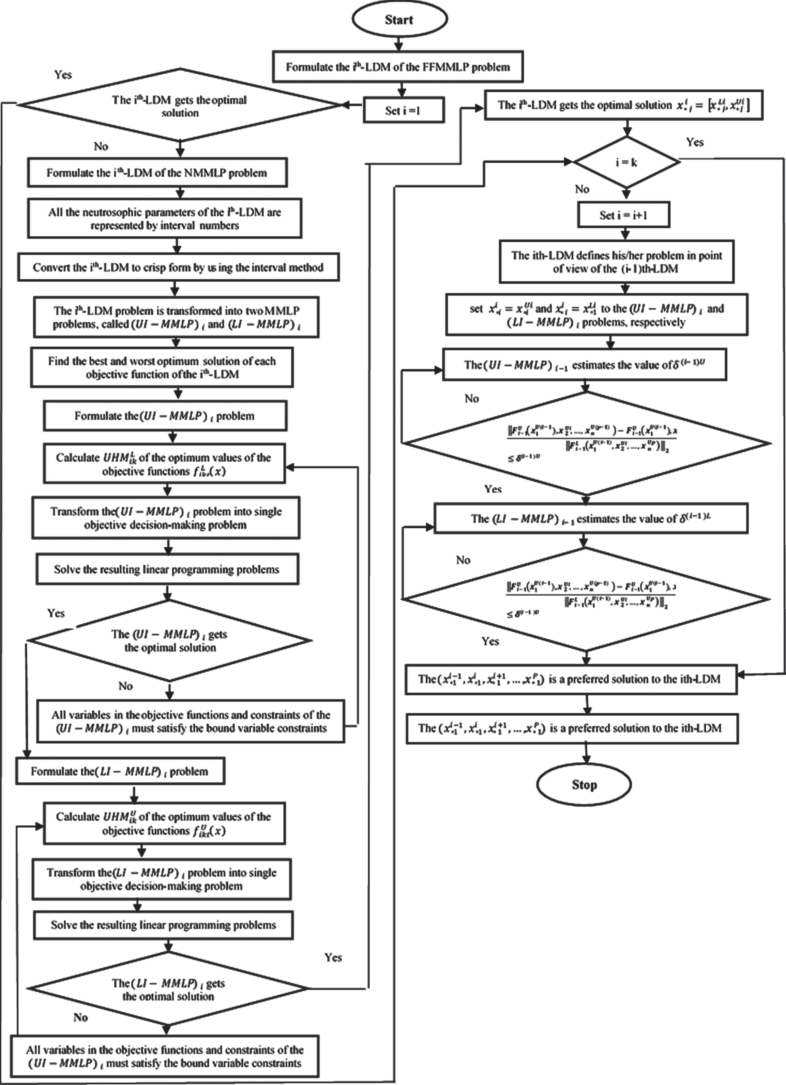
A flowchart depicting the suggested problem’s decision-making process.

6 Neutrosophic multi-objective transportation (NMOT) problem

This section proposes a new compromise approach for the multi-objective transportation (NMOT) problem, based on the harmonic mean technique, where the transportation cost, supply, and demand are all represented by neutrosophic numbers.

6.1 Mathematical model of (NMMTP) problem

NMOT problem is concerned with moving a product from k sources (s₁, s₂, …, s_k) to n destinations (d₁, d₂, …, d_n) while meeting r objectives $(f_{1}^{N} (x), f_{2}^{N} (x), \dots, f_{r}^{N} (x))$ . Each source s_i has available supply, $a_{i}^{N}$ , (i = 1, 2, …, k), and each destination d_j, (j = 1, 2, …, n), has a specific level of demand. Furthermore, transferring a unit from source s_i to destination d_j incurs a penalty $c_{ij}^{(s) N}$ for the objective $f_{s}^{N} (x)$ , (s = 1, 2, …, r). The corresponding penalty could be shipping costs, delivery time, or delivery safety, for example. Under the optimization aspect, the solution to this problem is to determine an unknown quantity of products, x_ij, that were shipped from source s_i to destination d_j. The mathematical formulation of the NMOT problem can be described as follows using this description:

$min F^{N} (x) = (f_{1}^{N} (x), \dots, f_{r}^{N} (x)) = (\sum_{j = 1}^{n} \sum_{i = 1}^{k} c_{ij}^{(1) N} x_{ij}, \dots, \sum_{j = 1}^{n} \sum_{i = 1}^{k} c_{ij}^{(r) N} x_{ij})$ ,

subject to

$G^{N} = {x \in R^{n} | \begin{matrix} \sum_{j = 1}^{n} x_{ij} = a_{i}^{N}, (i = 1, 2, \dots, k) \\ \sum_{i = 1}^{k} x_{ij} = b_{j}^{N}, (j = 1, 2, \dots, n) \\ x_{ij} ⩾ 0 \end{matrix}}$ (37)

Allow interval numbers to be used to represent all of the neotrosophic numbers in Problem (37):

$\begin{matrix} c_{ij}^{(s) N} = c_{ij}^{s} + d_{ij}^{s} I_{ij}^{s} = c_{ij}^{s} + d_{ij}^{s} [I_{ij}^{(s) L}, I_{ij}^{(s) U}] \\ = [c_{ij}^{s} + d_{ij}^{s} I_{ij}^{(s) L}, c_{ij}^{s} + d_{ij}^{s} I_{ij}^{(s) U}] = [c_{ij}^{(s) L}, c_{ij}^{(s) U}] \end{matrix}$ ,

$\begin{matrix} a_{i}^{N} = a_{i} + λ_{i} I_{i} = a_{i} + λ_{i} [I_{i}^{L}, I_{i}^{U}] \\ = [a_{i} + λ_{i} I_{i}^{L}, a_{i} + λ_{i} I_{i}^{U}] = [a_{i}^{L}, a_{i}^{U}] \end{matrix}$ ,

$\begin{matrix} b_{j}^{N} = b_{j} + μ_{j} I_{j} = b_{j} + μ_{j} [I_{j}^{L}, I_{j}^{U}] \\ = [b_{j} + μ_{j} I_{j}^{L}, b_{j} + μ_{j} I_{j}^{U}] = [b_{j}^{L}, b_{j}^{U}] \end{matrix}$

Where a_i, b_j, $c_{ij}^{s}$ , $d_{ij}^{s}$ , λ_i, and μ_j are real numbers, (i = 1, 2, …, k ; j = 1, 2, …, n ; s = 1, 2, …, r).

As a result, Problem (37) can be rewritten as follows:

$min F^{N} (x) = (\sum_{j = 1}^{n} \sum_{i = 1}^{k} [c_{ij}^{(1) L}, c_{ij}^{(1) U}] x_{ij}, \dots,$

$\sum_{j = 1}^{n} \sum_{i = 1}^{k} [c_{ij}^{(r) L}, c_{ij}^{(r) U}] x_{ij})$

subject to

$G^{N} = {x \in R^{n} | \begin{matrix} \sum_{j = 1}^{n} x_{ij} = [a_{i}^{L}, a_{i}^{U}], (i = 1, 2, \dots, k) \\ \sum_{i = 1}^{k} x_{ij} = [b_{j}^{L}, b_{j}^{U}], (j = 1, 2, \dots, n) \\ x_{ij} ⩾ 0 \end{matrix}}$ (38)

Definition 7. The neotrosophic transportation problem is called the balanced neotrosophic transportation problem if $\sum_{i = 1}^{k} a_{i}^{L} = \sum_{j = 1}^{n} b_{j}^{L}$ and $\sum_{i = 1}^{k} a_{i}^{U} = \sum_{j = 1}^{n} b_{j}^{U}$ ; otherwise, it is called an unbalanced neotrosophic transportation problem.

6.2 A solution strategy for the NMOT problem

An NMOT problem is broken into the following two crisp multi-objective transportation problems, which are solved using classic transportation simplex algorithms, according to the methodology established in Subsection 3.2.

$P^{L} : min F^{L} (x) = (\sum_{j = 1}^{n} \sum_{i = 1}^{k} c_{ij}^{(1) L} x_{ij}, \dots, \sum_{j = 1}^{n} \sum_{i = 1}^{k} c_{ij}^{(r) L} x_{ij})$ ,

subject to

$G^{L} = {x \in R^{n} | \begin{matrix} \sum_{j = 1}^{n} x_{ij} = a_{i}^{L}, (i = 1, 2, \dots, k) \\ \sum_{i = 1}^{k} x_{ij} = b_{j}^{L}, (j = 1, 2, \dots, n) \\ x_{ij} ⩾ 0 \end{matrix}}$ (39)

$P^{U} : min F^{U} (x) = (\sum_{j = 1}^{n} \sum_{i = 1}^{k} c_{ij}^{(1) U} x_{ij}, \dots, \sum_{j = 1}^{n} \sum_{i = 1}^{k} c_{ij}^{(r) U} x_{ij})$ ,

subject to

$G^{U} = {x \in R^{n} | \begin{matrix} \sum_{j = 1}^{n} x_{ij} = a_{i}^{U}, (i = 1, 2, \dots, k) \\ \sum_{i = 1}^{k} x_{ij} = b_{j}^{U}, (j = 1, 2, \dots, n) \\ x_{ij} ⩾ 0 \end{matrix}}$ (40)

Find the individual optimum solutions for each objective function, as follows:

$\begin{matrix} f_{s}^{* U} = min_{x \in G^{U}} \sum_{j = 1}^{n} \sum_{i = 1}^{k} c_{ij}^{(s) U} x_{ij}, \\ f_{s}^{* L} = min_{x \in G^{L}} \sum_{j = 1}^{n} \sum_{i = 1}^{k} c_{ij}^{(s) L} x_{ij} (s = 1, 2, \dots, r) \end{matrix}$ (41)

Calculate the UHM^L and UHM^U of the optimum values of the objective functions $f_{s}^{* L}$ and $f_{s}^{* U}$ , respectively. As a result:

$\begin{matrix} UHM = [{UHM}^{L}, {UHM}^{U}] \\ = [\frac{r}{\sum_{s = 1}^{r} (\frac{1}{f_{s}^{* L}})}, \frac{r}{\sum_{s = 1}^{r} (\frac{1}{f_{s}^{* U}})}] \end{matrix}$ (42)

UHM^L and UHM^U, can have positive or negative values. If they’re negative, we look at the absolute values of UHM^L and UHM^U.

To arrive at the optimal solution, we apply the harmonic mean technique to reduce the NMOT problem into the following single-objective transportation problems.

${STP}^{L} : min F^{L} (x) = \frac{\sum_{s = 1}^{r} (min_{x \in G^{L}} \sum_{j = 1}^{n} \sum_{i = 1}^{k} c_{ij}^{(s) L} x_{ij})}{{UHM}^{U}},$

subject to

$x \in G^{L}$ (43)

${STP}^{U} : min F^{U} (x) = \frac{\sum_{s = 1}^{r} (min_{x \in G^{L}} \sum_{j = 1}^{n} \sum_{i = 1}^{k} c_{ij}^{(s) U} x_{ij})}{{UHM}^{L}},$

subject to

$x \in G^{U}$ (44)

The optimal interval solution of the neutrosophic multi-objective transportation problem is x^*I = [x^*L, x^*U] when solving the two crisp transportation problems, STP^L and STP^U, one at a time using normal transportation simplex algorithms. F^*I (x^*I) is the optimal interval minimum transportation cost.

7 Numerical examples

To demonstrate the computational technique, we first explore a hypothetical case, followed by two examples for addressing a neutrosophic multi-objective transportation problem. It is assumed that I ∈ [0, 1] in these examples.

Example 7.1.

Consider the following neotrosophic three-level multi-objective linear programming problem.

FLDM:

$max_{x_{1}} f_{11} = [3 + 4 I] x_{1} + [6 + 8 I] x_{2} + [4 + 2 I] x_{3} + [1 + 3 I]$

$max_{x_{1}} f_{12} = [14 + 2 I] x_{1} + [5 + 3 I] x_{2} + [2 - I] x_{3} + [6 + 6 I]$

$min_{x_{1}} f_{13} = [1 + 2 I] x_{1} + [2 + I] x_{2} + [1 + I] x_{3} + [20 + 13 I]$

SLDM:

$max_{x_{2}} f_{21} = [1 + I] x_{1} + [5 + 9 I] x_{2} - [2 + 3 I] x_{3} + [6 + 11 I]$

$max_{x_{2}} f_{22} = [3 - 2 I] x_{1} + [7 + 10 I] x_{2} + [4 + 8 I] x_{3} + [14 + 5 I]$

$max_{x_{2}} f_{23} = [2 + 2 I] x_{1} + [4 + 11 I] x_{2} + [6 + 3 I] x_{3} + [3 + 7 I]$

TLDM:

$max_{x_{3}} f_{31} = [- 2 + 3 I] x_{1} + [9 + 5 I] x_{2} + [10 + 6 I] x_{3} + [4 + 7 I]$

$max_{x_{3}} f_{32} = [8 + 13 I] x_{1} + [1 + 3 I] x_{2} + [12 + 15 I] x_{3} + [2 + 4 I]$

$min_{x_{3}} f_{33} = [5 + I] x_{1} - [3 + 7 I] x_{2} + [8 + 13 I] x_{3} + [5 + 8 I]$

subject to

[2 + 2I] x₁ + [2 + I] x₂ + [1 + I] x₃ ⩽ [10 + 7I]

[1 + 2I] x₁ + [1 + 4I] x₂ + [2 + I] x₃ ⩽ [8 + 10I]

x₁, x₂, x₃ ⩾ 0

The first stage in the solution technique is to change the original NMMLP problem into an MMLP problem with crisp coefficients and crisp decision variables using the arithmetic operations defined in Definitions 2 and 4.

To begin, the FLDM can be rewritten as follows:

The following is the problem for which the best solution is sought:

$max_{x_{1}} f_{11}^{L} = 3 x_{1} + 6 x_{2} + 4 x_{3} + 1$

$max_{x_{1}} f_{12}^{L} = 14 x_{1} + 5 x_{2} + x_{3} + 6$

$min_{x_{1}} f_{13}^{L} = x_{1} + 2 x_{2} + x_{3} + 20$

subject to

2x₁ + 2x₂ + x₃ ⩽ 10

x₁ + x₂ + 2x₃ ⩽ 8

x₁, x₂, x₃ ⩾ 0

The following is a problem with the worst possible solution:

$max_{x_{1}} f_{11}^{U} = 7 x_{1} + 14 x_{2} + 6 x_{3} + 4$

$max_{x_{1}} f_{12}^{U} = 16 x_{1} + 8 x_{2} + 2 x_{3} + 12$

$min_{x_{1}} f_{13}^{U} = 3 x_{1} + 3 x_{2} + 2 x_{3} + 33$

subject to

4x₁ + 3x₂ + 2x₃ ⩽ 20

3x₁ + 5x₂ + 2x₃ ⩽ 30

x₁, x₂, x₃ ⩾ 0

Table 1 shows the individual optimal solutions for the decision variables and the FLDM’s objective functions.

Table 1
Individual optimal solutions for the FLDM problems

FLDM

$f_{11}^{L}$ $f_{12}^{L}$ $f_{13}^{L}$ $f_{11}^{U}$ $f_{12}^{U}$ $f_{13}^{U}$

x ₁ 0 5 0 0 5 0

x ₂ 4 0 0 5 0 0

x ₃ 2 0 0 2.5 0 0

Optimal solution 33 76 20 89 92 33

SLDM

$f_{21}^{L}$ $f_{22}^{L}$ $f_{23}^{L}$ $f_{21}^{U}$ $f_{22}^{U}$ $f_{23}^{U}$

x ₁ 5 5 5 5 5 5

x ₂ 0 0 0 0 0 0

x ₃ 0 0 0 0 0 0

Optimal solution 11 19 13 27 34 30

TLDM

$f_{31}^{L}$ $f_{32}^{L}$ $f_{33}^{L}$ $f_{31}^{U}$ $f_{32}^{U}$ $f_{33}^{U}$

x ₁ 5 5 5 5 5 5

x ₂ 0 0 0 0 0 0

x ₃ 0 0 0 0 0 0

Optimal solution -6 42 30 16 111 43

Calculate the ${UHM}_{11}^{L}$ , ${UHM}_{12}^{L}$ , ${UHM}_{11}^{U}$ and ${UHM}_{12}^{U}$ of the optimum values of the objective functions $f_{1 k}^{L} (x)$ , $f_{1 k}^{U} (x)$ , (k = 1, 2), of FLDM problems, respectively. Such that ${UHM}_{11}^{L} = 46.0183$ , ${UHM}_{12}^{L} = 20$ , ${UHM}_{11}^{U} = 90.4751$ and ${UHM}_{12}^{U} = 33$ .

The FLDM problems’ equivalent single objective function can be written as follows:

The following is the problem for which the best solution is sought:

$max_{x_{1}} F_{1}^{L} = 0.1576 x_{1} + 0.061 x_{2} - 0.025 x_{3} - 0.377$

subject to

2x₁ + 2x₂ + x₃ ⩽ 10

x₁ + x₂ + 2x₃ ⩽ 8

x₁, x₂, x₃ ⩾ 0

The following is a problem with the worst possible solution:

$max_{x_{1}} F_{1}^{U} = 0.349 x_{1} + 0.328 x_{2} + 0.0738 x_{3} - 1.302$

subject to

4x₁ + 3x₂ + 2x₃ ⩽ 20

3x₁ + 5x₂ + 2x₃ ⩽ 30

x₁, x₂, x₃ ⩾ 0

As a result, the optimal FLDM solution is [0.4108, 0.4467], with $x_{1}^{F} = [5, 5],$ $x_{2}^{F} = [0, 0]$ and $x_{3}^{F} = [0, 0]$ . Let δ^F = 0.1, where δ^F is a constant given by the FLDM and is a sufficiently small positive number.

SLDM constraints should now have $x_{1}^{F} = [5, 5]$ . Following that, here are the SLDM problems:

The following is the problem that needs to be solved in order to get the best solution:

$max_{x_{2}} f_{21}^{L} = x_{1} + 5 x_{2} - 5 x_{3} + 6$

$max_{x_{2}} f_{22}^{L} = x_{1} + 7 x_{2} + 4 x_{3} + 14$

$max_{x_{2}} f_{23}^{L} = 2 x_{1} + 4 x_{2} + 6 x_{3} + 3$

subject to

2x₁ + 2x₂ + x₃ ⩽ 10

x₁ + x₂ + 2x₃ ⩽ 8

x₁ = 5

x₂, x₃ ⩾ 0 .

The problem for the worst solution is as follows:

$max_{x_{2}} f_{21}^{U} = 2 x_{1} + 14 x_{2} - 2 x_{3} + 17$

$max_{x_{2}} f_{22}^{U} = 3 x_{1} + 17 x_{2} + 12 x_{3} + 19$

$max_{x_{2}} f_{23}^{U} = 4 x_{1} + 15 x_{2} + 9 x_{3} + 10$

subject to

4x₁ + 3x₂ + 2x₃ ⩽ 20

3x₁ + 5x₂ + 2x₃ ⩽ 30

x₁ = 5

x₂, x₃ ⩾ 0

Table 1 shows the individual optimal solutions for the decision variables and the SLDM’s objective functions.

The SLDM follows the same steps as the FLDM to arrive at the following results: the SLDM problem’s optimal solution is [1.4302, 6.6874], where $x_{1}^{F} = [5, 5]$ , $x_{2}^{S} = [0, 0]$ , and $x_{3}^{S} = [0, 0] .$

Now, the FLDM uses the FLDM satisfactoriness test function to determine whether the proposed solution $(x_{1}^{F}, x_{2}^{S}, x_{3}^{S})$ is a preferred and acceptable option to him/her, or whether it should be amended.

$\frac{{∥ F_{1}^{L} (5, 0, 0) - F_{1}^{L} (5, 0, 0) ∥}_{2}}{{∥ F_{1}^{L} (5, 0, 0) ∥}_{2}} = 0 < δ^{F}$ ,

$\frac{{∥ F_{1}^{U} (5, 0, 0) - F_{1}^{U} (5, 0, 0) ∥}_{2}}{{∥ F_{1}^{U} (5, 0, 0) ∥}_{2}} = 0 < δ^{F}$ ,

As a result, the FLDM solution $(x_{1}^{F}, x_{2}^{S}, x_{3}^{S})$ is preferred. The SLDM gives the constant δ^S = 0.1, where δ^S is a small positive number.

Set $x_{1}^{F} = [5, 5]$ and $x_{2}^{S} = [0, 0]$ to the TLDM constraints. The TLDM problems are then written as follows:

The following is the problem for which the best solution is sought:

$max_{x_{3}} f_{31}^{L} = x_{1} + 5 x_{2} - 5 x_{3} + 6$

$max_{x_{3}} f_{32}^{L} = x_{1} + 7 x_{2} + 4 x_{3} + 14$

$min_{3} f_{33}^{L} = 2 x_{1} + 4 x_{2} + 6 x_{3} + 3$

subject to

2x₁ + 2x₂ + x₃ ⩽ 10

x₁ + x₂ + 2x₃ ⩽ 8

x₁ = 5, x₂ = 0

x₃ ⩾ 0.

The following is a problem with the worst possible solution:

$max_{x_{3}} f_{31}^{U} = 2 x_{1} + 14 x_{2} - 2 x_{3} + 17$

$max_{x_{3}} f_{32}^{U} = 3 x_{1} + 17 x_{2} + 12 x_{3} + 19$

$min_{x_{3}} f_{33}^{U} = 4 x_{1} + 15 x_{2} + 9 x_{3} + 10$

subject to

4x₁ + 3x₂ + 2x₃ ⩽ 20

3x₁ + 5x₂ + 2x₃ ⩽ 30

x₁ = 5, x₂ = 0

x₃ ⩾ 0.

Table 1 shows the individual optimal solutions for the decision variables and the TLDM’s objective functions.

The TLDM follows the same steps as the FLDM to achieve the following outcomes:

The TLDM problem’s optimal solution is [0.5895, 7.6381], where $x_{3}^{T} = [0, 0]$ .

Now, the SLDM uses the SLDM satisfactoriness test function to determine whether the offered solution $(x_{1}^{F}, x_{2}^{S}, x_{3}^{T})$ is a preferred and acceptable option to him/her, or whether it should be adjusted. $\frac{{∥ f_{2}^{L} (5, 0, 0) - f_{2}^{L} (5, 0, 0) ∥}_{2}}{{∥ f_{2}^{L} (5, 0, 0) ∥}_{2}} = 0 < δ^{S},$ $\frac{{∥ f_{2}^{U} (5, 0, 0) - f_{2}^{U} (5, 0, 0) ∥}_{2}}{{∥ f_{2}^{U} (5, 0, 0) ∥}_{2}} = 0 < δ^{S} .$

As a result, $(x_{1}^{F}, x_{2}^{S}, x_{3}^{T})$ is the preferred SLDM solution. As a consequence, F^F = [0.4108, 0.4467], F^S = [1.4302, 6.6874], and F^T = [0.5895, 7.6381] are preferred solutions for the NMMLP problem, with optimal decision variables $x_{1}^{F} = [5, 5]$ , $x_{2}^{S} = [0, 0]$ , and $x_{3}^{T} = [0, 0]$ .

Example 7.2.

Consider the following features of a balanced neutrosophic multi-objective transportation (NMOT) problem:

Supplies:

$a_{1}^{N} = [18 + 9 I]$ , $a_{2}^{N} = [20 + 17 I]$ , $a_{3}^{N} = [13 + 6 I]$ .

Demands:

$b_{1}^{N} = [10 + 4 I]$ , $b_{2}^{N} = [12 + 8 I]$ , $b_{3}^{N} = [14 + 7 I]$ , $b_{4}^{N} = [15 + 13 I]$ .

Costs:

$c_{1}^{N} = (\begin{matrix} \begin{matrix} [3 + 2 I] & [1 + 4 I] & [2 + 2 I] \end{matrix} & [5 + I] \\ \begin{matrix} \begin{matrix} [1 + 7 I] \\ [7 + 4 I] \end{matrix} & \begin{matrix} [3 + 6 I] \\ [5 + 2 I] \end{matrix} & \begin{matrix} [4 + 5 I] \\ [6 + 8 I] \end{matrix} \end{matrix} & \begin{matrix} [3 + 2 I] \\ [4 + I] \end{matrix} \end{matrix})$ ,

$c_{2}^{N} = (\begin{matrix} \begin{matrix} [8 + 3 I] & [2 + 7 I] & [4 + I] \end{matrix} & [3 + 5 I] \\ \begin{matrix} \begin{matrix} [1 + 6 I] \\ [6 + 5 I] \end{matrix} & \begin{matrix} [3 + 4 I] \\ [1 + 2 I] \end{matrix} & \begin{matrix} [2 + 8 I] \\ [8 + 9 I] \end{matrix} \end{matrix} & \begin{matrix} [7 + 7 I] \\ [5 + 4 I] \end{matrix} \end{matrix})$

$c_{3}^{N} = (\begin{matrix} \begin{matrix} [9 + I] & [3 + 7 I] & [1 + I] \end{matrix} & [6 + 4 I] \\ \begin{matrix} \begin{matrix} [4 + 8 I] \\ [2 + 5 I] \end{matrix} & \begin{matrix} [5 + 6 I] \\ [3 + 9 I] \end{matrix} & \begin{matrix} [5 + 7 I] \\ [6 + 3 I] \end{matrix} \end{matrix} & \begin{matrix} [8 + 2 I] \\ [7 + 2 I] \end{matrix} \end{matrix})$

An NMOT problem is broken into the following two crisp balanced multi-objective transportation problems:

P^L : min F^L (x) = (3x₁₁ + x₁₂ + 2x₁₃ + 5x₁₄ + x₂₁ + 3x₂₂ + 4x₂₃ +3x₂₄ + 7x₃₁ + 5x₃₂ + 6x₃₃ + 4x₃₄, 8x₁₁ +2x₁₂ + 4x₁₃ + 3x₁₄ + x₂₁ + 3x₂₂ + 2x₂₃ +7x₂₄ + 6x₃₁ + x₃₂ + 8x₃₃ + 5x₃₄, 9x₁₁ +3x₁₂ + x₁₃ + 6x₁₄ + 4x₂₁ + 5x₂₂ + 5x₂₃ +8x₂₄ + 2x₃₁ + 3x₃₂ + 6x₃₃ + 7x₃₄),

subject to

G^L = {x₁₁ + x₁₂ + x₁₃ + x₁₄ = 18

x₂₁ + x₂₂ + x₂₃ + x₂₄ = 20

x₃₁ + x₃₂ + x₃₃ + x₃₄ = 13

x₁₁ + x₂₁ + x₃₁ = 10

x₁₂ + x₂₂ + x₃₂ = 12

x₁₃ + x₂₃ + x₃₃ = 14

x₁₄ + x₂₄ + x₃₄ = 15

x_ij ⩾ 0, (i = 1, 2, 3 ; j = 1, 2, 3, 4)}.

P^U : minF^U (x) = (5x₁₁ + 5x₁₂ +4x₁₃ + 6x₁₄ + 8x₂₁ + 9x₂₂ + 9x₂₃ + 5x₂₄ + 11x₃₁ +7x₃₂ + 14x₃₃ + 5x₃₄, 11x₁₁ + 9x₁₂ + 5x₁₃ + 8x₁₄ + 7x₂₁ + 7x₂₂ + 10x₂₃ + 14x₂₄ + 11x₃₁ +3x₃₂ + 17x₃₃ + 9x₃₄, 10x₁₁ + 10x₁₂ +2x₁₃ + 10x₁₄ +12x₂₁ + 11x₂₂ + 12x₂₃ +10x₂₄ + 7x₃₁ + 12x₃₂ + 9x₃₃ + 9x₃₄) ,

subject to

G^U = {x₁₁ + x₁₂ + x₁₃ + x₁₄ = 27

x₂₁ + x₂₂ + x₂₃ + x₂₄ = 37

x₃₁ + x₃₂ + x₃₃ + x₃₄ = 19

x₁₁ + x₂₁ + x₃₁ = 14

x₁₂ + x₂₂ + x₃₂ = 20

x₁₃ + x₂₃ + x₃₃ = 21

x₁₄ + x₂₄ + x₃₄ = 28

x_ij ⩾ 0, (i = 1, 2, 3 ; j = 1, 2, 3, 4)}.

Table 2 shows the individual optimal solutions for the decision variables and the balanced NMOT problem’s objective functions.

Table 2

Individual optimal solutions for the balanced NMOT problem

	$f_{1}^{L}$	$f_{2}^{L}$	$f_{3}^{L}$	$f_{1}^{U}$	$f_{2}^{U}$	$f_{3}^{U}$
x ₁₁	0	0	0	5	0	0
x ₁₂	4	0	0	1	0	6
x ₁₃	14	4	14	21	18	21
x ₁₄	0	14	4	0	9	0
x ₂₁	10	10	0	9	14	0
x ₂₂	8	0	9	0	20	14
x ₂₃	0	10	0	0	3	0
x ₂₄	2	0	11	28	0	23
x ₃₁	0	0	10	0	0	14
x ₃₂	0	12	3	19	0	0
x ₃₃	0	0	0	0	0	0
x ₃₄	13	1	0	0	19	5
Optimal solution	124	105	200	459	601	629

Calculate the UHM^L and UHM^U of the optimum values of the objective functions $f_{s}^{* L}$ and $f_{s}^{* U}$ , (s = 1, 2, 3), respectively. As a result, UHM^L = 132.812 and UHM^U = 552.2454.

We apply the harmonic mean technique to reduce the NMOT problem into the following balanced single-objective transportation problems.

$\begin{matrix} {STP}^{L} : min F^{L} (x) = (0.0362 x_{11} + 0.0109 x_{12} \\ + 0.0127 x_{13} + 0.0254 x_{14} + 0.0109 x_{21} \\ + 0.0199 x_{22} + 0.0199 x_{23} + 0.0326 x_{24} \\ + 0.0272 x_{31} + 0.0163 x_{32} + 0.0362 x_{33} \\ + 0.029 x_{34} \end{matrix}$ ,

subject to

x ∈ G^L

$\begin{matrix} {STP}^{U} : min F^{U} (x) = (0.1958 x_{11} + 0.1807 x_{12} \\ + 0.0828 x_{13} + 0.1807 x_{14} + 0.2033 x_{21} \\ + 0.2033 x_{22} + 0.2334 x_{23} + 0.2184 x_{24} \\ + 0.2184 x_{31} + 0.1656 x_{32} + 0.3012 x_{33} \\ + 0.1732 x_{34} \end{matrix}$ ,

subject to

x ∈ G^U

The optimal interval solution of the balanced neutrosophic multi-objective transportation problem is $x_{11}^{*} = [0, 0]$ , $x_{12}^{*} = [0, 0]$ , $x_{13}^{*} = [12, 19]$ , $x_{14}^{*} = [6, 8]$ , $x_{21}^{*} = [10, 14]$ , $x_{22}^{*} = [1, 3]$ , $x_{23}^{*} = [0, 0]$ , $x_{24}^{*} = [9, 20]$ , $x_{31}^{*} = [0, 0]$ , $x_{32}^{*} = [11, 17]$ , $x_{33}^{*} = [2, 2]$ , and $x_{34}^{*} = [0, 0]$ . F^* = [0.9788, 14.2605] is the optimal interval minimum transportation cost.

Example 7.3.

Consider the following features of an unbalanced NMOT problem:

Supplies:

$a_{1}^{N} = [9 + 3 I]$ , $a_{2}^{N} = [5 + 11 I]$ , $a_{3}^{N} = [21 + 8 I]$ .

Demands:

$b_{1}^{N} = [13 + 5 I]$ , $b_{2}^{N} = [10 + 2 I]$ , $b_{3}^{N} = [5 + 2 I]$ , $b_{4}^{N} = [7 + 13 I]$ .

Costs:

$c_{1}^{N} = (\begin{matrix} \begin{matrix} [4 + 3 I] & [2 + 4 I] & [1 + 7 I] \end{matrix} & [8 + 2 I] \\ \begin{matrix} \begin{matrix} [3 + 2 I] \\ [6 + 5 I] \end{matrix} & \begin{matrix} [1 + 7 I] \\ [5 + 5 I] \end{matrix} & \begin{matrix} [6 + 4 I] \\ [7 + I] \end{matrix} \end{matrix} & \begin{matrix} [2 + 3 I] \\ [4 + 6 I] \end{matrix} \end{matrix})$ ,

$c_{2}^{N} = (\begin{matrix} \begin{matrix} [6 + 2 I] & [1 + 5 I] & [3 + 4 I] \end{matrix} & [4 + 2 I] \\ \begin{matrix} \begin{matrix} [7 + 3 I] \\ [5 + 4 I] \end{matrix} & \begin{matrix} [9 + 6 I] \\ [4 + 5 I] \end{matrix} & \begin{matrix} [6 + 3 I] \\ [2 + 9 I] \end{matrix} \end{matrix} & \begin{matrix} [6 + 4 I] \\ [7 + 8 I] \end{matrix} \end{matrix})$

$c_{3}^{N} = (\begin{matrix} \begin{matrix} [8 + 2 I] & [6 + I] & [4 + 3 I] \end{matrix} & [7 + 2 I] \\ \begin{matrix} \begin{matrix} [5 + 4 I] \\ [3 + 3 I] \end{matrix} & \begin{matrix} [6 + 2 I] \\ [2 + 7 I] \end{matrix} & \begin{matrix} [9 + I] \\ [5 + 8 I] \end{matrix} \end{matrix} & \begin{matrix} [8 + I] \\ [4 + 5 I] \end{matrix} \end{matrix})$

An unbalanced NMOT problem is broken into the following two crisp unbalanced multi-objective transportation problems:

P^L : min F^L (x) = (4x₁₁ + 2x₁₂ + x₁₃ + 8x₁₄ +3x₂₁ + x₂₂ + 6x₂₃ + 2x₂₄ + 6x₃₁ + 5x₃₂ + 7x₃₃ +4x₃₄, 6x₁₁ + x₁₂ + 3x₁₃ + 4x₁₄ + 7x₂₁ + 9x₂₂ +6x₂₃ + 6x₂₄ + 5x₃₁ + 4x₃₂ + 2x₃₃ + 7x₃₄, 8x₁₁ +6x₁₂ + 4x₁₃ + 7x₁₄ + 5x₂₁ + 6x₂₂ + 9x₂₃ + 8x₂₄ +3x₃₁ + 2x₃₂ + 5x₃₃ + 4x₃₄)

subject to

x₁₁ + x₁₂ + x₁₃ + x₁₄ = 9

x₂₁ + x₂₂ + x₂₃ + x₂₄ = 5

x₃₁ + x₃₂ + x₃₃ + x₃₄ = 21

x₁₁ + x₂₁ + x₃₁ = 13

x₁₂ + x₂₂ + x₃₂ = 10

x₁₃ + x₂₃ + x₃₃ = 5

x₁₄ + x₂₄ + x₃₄ = 7

x_ij ⩾ 0, (i = 1, 2, 3 ; j = 1, 2, 3, 4).

P^U : minF^U (x) = (7x₁₁ + 6x₁₂ + 8x₁₃ +10x₁₄ + 5x₂₁ + 8x₂₂ + 10x₂₃ + 5x₂₄ +11x₃₁ + 10x₃₂ + 8x₃₃ + 10x₃₄, 8x₁₁ +6x₁₂ + 7x₁₃ + 6x₁₄ + 10x₂₁ + 15x₂₂ +9x₂₃ + 10x₂₄ + 9x₃₁ + 9x₃₂ + 11x₃₃ +15x₃₄, 10x₁₁ + 7x₁₂ + 7x₁₃ + 9x₁₄ +9x₂₁ + 8x₂₂ + 10x₂₃ + 9x₂₄ + 6x₃₁ +9x₃₂ + 13x₃₃ + 9x₃₄) ,

subject to

x₁₁ + x₁₂ + x₁₃ + x₁₄ = 12

x₂₁ + x₂₂ + x₂₃ + x₂₄ = 16

x₃₁ + x₃₂ + x₃₃ + x₃₄ = 29

x₁₁ + x₂₁ + x₃₁ = 18

x₁₂ + x₂₂ + x₃₂ = 12

x₁₃ + x₂₃ + x₃₃ = 7

x₁₄ + x₂₄ + x₃₄ = 20

x_ij ⩾ 0, (i = 1, 2, 3 ; j = 1, 2, 3, 4).

Table 3 shows the individual optimal solutions for the decision variables and the unbalanced NMOT problem’s objective functions.

Table 3

Individual optimal solutions for the unbalanced NMOT problem

	$f_{1}^{L}$	$f_{2}^{L}$	$f_{3}^{L}$	$f_{1}^{U}$	$f_{2}^{U}$	$f_{3}^{U}$
x ₁₁	0	0	0	0	0	0
x ₁₂	4	9	0	12	1	5
x ₁₃	5	0	5	0	0	7
x ₁₄	0	0	4	0	11	0
x ₂₁	0	0	5	16	0	0
x ₂₂	5	0	0	0	0	7
x ₂₃	0	0	0	0	7	0
x ₂₄	0	5	0	0	9	9
x ₃₁	13	13	8	2	18	18
x ₃₂	1	1	10	0	11	0
x ₃₃	0	5	0	7	0	0
x ₃₄	7	2	3	20	0	11
Optimal solution	129	132	129	430	486	428

Calculate the UHM^L and UHM^U of the optimum values of the objective functions $f_{s}^{* L}$ and $f_{s}^{* U}$ , (s = 1, 2, 3), respectively. As a result, UHM^L = 129.9847 and UHM^U = 446.4523.

We apply the harmonic mean technique to reduce the NMOT problem into the following unbalanced single-objective transportation problems.

$\begin{matrix} {STP}^{L} : min F^{L} (x) = (0.0403 x_{11} + 0.0202 x_{12} \\ + 0.0179 x_{13} + 0.0426 x_{14} + 0.0336 x_{21} \\ + 0.0358 x_{22} + 0.047 x_{23} + 0.0358 x_{24} \\ + 0.0314 x_{31} + 0.0246 x_{32} + 0.0314 x_{33} \\ + 0.0336 x_{34} \end{matrix}$ ,

subject to

x ∈ G^L

$\begin{matrix} {STP}^{U} : min F^{U} (x) = (0.1923 x_{11} + 0.1462 x_{12} \\ + 0.1693 x_{13} + 0.1923 x_{14} + 0.1846 x_{21} \\ + 0.2385 x_{22} + 0.2231 x_{23} + 0.1846 x_{24} \\ + 0.2 x_{31} + 0.2154 x_{32} + 0.2462 x_{33} \\ + 0.2616 x_{34} \end{matrix}$ ,

subject to

x ∈ G^U

The optimal interval solution of the unbalanced neutrosophic multi-objective transportation problem is $x_{11}^{*} = [0, 0]$ , $x_{12}^{*} = [0, 0]$ , $x_{13}^{*} = [5, 7]$ , $x_{14}^{*} = [4, 5]$ , $x_{21}^{*} = [0, 0]$ , $x_{22}^{*} = [2, 2]$ , $x_{23}^{*} = [0, 0]$ , $x_{24}^{*} = [3, 14]$ , $x_{31}^{*} = [13, 18]$ , $x_{32}^{*} = [8, 10]$ , $x_{33}^{*} = [0, 0]$ , and $x_{34}^{*} = [0, 1]$ . F^* = [1.0439, 11.2236] is the optimal interval minimum transportation cost.

8 Conclusion

The neutrosophic multi-objective multi-level linear programming (NMMLP) problems were modelled using an interactive technique in this paper. Each neutrosophic problem was turned into two crisp multi-objective linear problems using the interval method in the proposed manner. The concept of harmonic means was then applied to combine the multiple objectives of each crisp problem into a single objective. Then, an interactive method for obtaining the preferred solution to the provided NMMLP problems has been devised. Finally, in a neutrosophic environment, an application to determine the optimality for the cost of multi-objective transportation problem is described. Numerical examples were presented to test the method’s validity.

References

Ammar

E.E.

and Khalifa

H.A.

, On fuzzy multi-objective multiitem solid transportation problems,1–19T, International Journal of Computer & Organization Trends 17 (2015).

Ammar

E.E.

and Youness

E.A.

, Study on multiobjective transportation problem with fuzzy numbers, Applied Mathematics and Computation 166 (2005), 241–253.

Arora

and Gupta

, Multi-level integer programming problem with multiple objectives at each level, Investigacion Operational 40 (2019), 313–329.

Banerjee

and Pramanik

, Single-objective linear goal programming problem with neutrosophic numbers, Infinite Study (2018).

Edalatpanah

S.A.

, A direct model for triangular neutrosophic linear programming, International Journal of Neutrosophic Science 1 (2020), 19–28.

Garg

and Rizk-Allah

R.M.

, A novel approach for solving rough multi-objective transportation problem: development and prospects, Computational and Applied Mathematics 40 (2021), 1–24.

Han

, Lu

and Zhang

, Tri-level decision-making for decentralized vendor-managed inventory, Information Sciences 421 (2017), 85–103.

Han

, Zhang

, Hu

and Lu

, A solution to bi/tri-level programming problems using particle swarm optimization, Information Sciences 370 (2016), 519–537.

Kouchakinejad

, Mashinchi

and Khorram

, Fuzzy multi-objective optimization of linear functions subject to max-arithmetic mean rational inequality constraints, Scientia Iranica 24 (2017), 1561–1570.

10.

Liu

and Liu

, The neutrosophic number generalized weighted power averaging operator and its application in multiple attribute group decision making, International Journal of Machine Learning and Cybernetics 9 (2018), 347–358.

11.

Liu

Q.M.

and Yang

Y.M.

, Interactive programming approach for solving multi-level multi-objective linear programming problem, Journal of Intelligent and Fuzzy Systems 35 (2018), 55–61.

12.

, Han

, Hu

and Zhang

, Multilevel decision-making: A survey, Information Sciences 346 (2016), 463–487.

13.

Mahmoudi

, Feylizadeh

M.R.

, Darvishi

and Liu

, Grey-fuzzy solution for multi-objective linear programming with interval coefficients, Grey Systems: Theory and Application (2018).

14.

Mondal

, Pramanik

, Giri

B.C.

and Smarandache

, NN-harmonic mean aggregation operators-based MCGDM strategy in a neutrosophic number environment, Axioms 7 (2018), 12.

15.

Moore

R.E.

and Yang

C.T.

, Interval analysis, Englewood-Cliffs, N J: Prentice-Hall (1996).

16.

Muruganadam

and Ambika

, Harmonic mean technique to solve multi objective fuzzy linear fractional programming problems, Global Journal of Pure and Applied Mathematics 13 (2017), 7321–7329.

17.

Osman

M.S.

, Abo-Sinna

M.A.

, Amer

A.H.

and Emam

, A multi-level non-linear multi-objective decision-making under fuzziness, Applied Mathematics and Computation 153 (2004), 239–252.

18.

Prabha

S.K.

, An innovative method to unravel neutroshopic transportation problem using harmonic mean, International Journal of Fuzzy System Applications (IJFSA) 10 (2021), 55–66.

19.

Pramanik

and Banerjee

, Neutrosophic number goal programming for multi-objective linear programming problem in neutrosophic number environment, Infinite Study (2018).

20.

Pramanik

and Dey

P.P.

, Multi-level linear programming problem with neutrosophic numbers: A goal programming strategy, Infinite Study (2019).

21.

Pramanik

and Mallick

, VIKOR based MAGDM strategy with trapezoidal neutrosophic numbers, Neutrosophic Sets and Systems 22 (2018), 118–129.

22.

Ramadan

, Linear programming with interval coefficients, Doctoral dissertation, Carleton University (1997).

23.

Sen

, A new approach for multi-objective rural development planning, The Indian Economic Journal 30 (1983), 91–96.

24.

Shaocheng, Interval number and fuzzy number linear programmings, Fuzzy Sets and Systems, 66 (1994), 301–306.

25.

Singh

, Arora

and Arora

, Bilevel transportation problem in neutrosophic environment, Computational and Applied Mathematics 41 (2022), 1–25.

26.

Smarandache

, A unifying field of logics, neutrosophy: Neutrosophic probability, set and logic, (1999), 1–141.

27.

Smarandache

, Introduction to neutrosophic measure, neutrosophic integral, and neutrosophic probability, Infinite Study (2013).

28.

Smarandache

and Khalid

H.E.

, Neutrosophic precalculus and neutrosophic calculus, Infinite Study (2018).

29.

Sohag

Z.I.

and Asadujjaman

, A proposed new average method for solving multi-objective linear programming problem using various kinds of mean techniques, Math Lett 4 (2018), 25–33.

30.

Sulaiman

N.A.

and Mustafa

R.B.

, Using harmonic mean to solve multi-objective linear programming problems, American Journal of Operations Research 6 (2016), 25–30.

31.

Sulaiman

N.A.

and Mustafa

R.B.

, Transform extreme point multi-objective linear programming problem to extreme point single objective linear programming problem by using harmonic mean, Applied Mathematics 6 (2016), 95–99.

32.

Veeramani

, Edalatpanah

S.A.

and Sharanya

, Solving the multiobjective fractional transportation problem through the neutrosophic goal programming approach, Discrete Dynamics in Nature and Society (2021).

33.

Wang

, Pesch

, Kress

, Fridman

and Boysen

, The piggyback transportation problem: transporting drones launched from a flying warehouse, European Journal of Operational Research 296 (2022), 504–519.

34.

, Fuzzy harmonic mean operators, International Journal of Intelligent Systems 24 (2009), 152–172.

	FLDM
	$f_{11}^{L}$	$f_{12}^{L}$	$f_{13}^{L}$	$f_{11}^{U}$	$f_{12}^{U}$	$f_{13}^{U}$
x ₁	0	5	0	0	5	0
x ₂	4	0	0	5	0	0
x ₃	2	0	0	2.5	0	0
Optimal solution	33	76	20	89	92	33
	SLDM
	$f_{21}^{L}$	$f_{22}^{L}$	$f_{23}^{L}$	$f_{21}^{U}$	$f_{22}^{U}$	$f_{23}^{U}$
x ₁	5	5	5	5	5	5
x ₂	0	0	0	0	0	0
x ₃	0	0	0	0	0	0
Optimal solution	11	19	13	27	34	30
	TLDM
	$f_{31}^{L}$	$f_{32}^{L}$	$f_{33}^{L}$	$f_{31}^{U}$	$f_{32}^{U}$	$f_{33}^{U}$
x ₁	5	5	5	5	5	5
x ₂	0	0	0	0	0	0
x ₃	0	0	0	0	0	0
Optimal solution	-6	42	30	16	111	43