Conflicting evidence combination based on Belief Mover’s Distance

Abstract

The Dempster-Shafer evidence theory has been extensively used in various applications of information fusion owing to its capability in dealing with uncertain modeling and reasoning. However, when meeting highly conflicting evidence, the classical Dempster’s combination rule may give counter-intuitive results. To address this issue, we propose a new method in this work to fuse conflicting evidence. Firstly, a new evidence distance metric, named Belief Mover’s Distance, which is inspired by the Earth Mover’s Distance, is defined to measure the difference between two pieces of evidence. Subsequently, the credibility weight and distance weight of each piece of evidence are computed according to the Belief Mover’s Distance. Then, the final weight of each piece of evidence is generated by unifying these two weights. Finally, the classical Dempster’s rule is employed to fuse the weighted average evidence. Several examples and applications are presented to analyze the performance of the proposed method. Experimental results manifest that the proposed method is remarkably effective in comparison with other methods.

Keywords

Evidence theory conflicting evidence combination rule evidence distance Belief Mover’s Distance

1 Introduction

Dempster-Shafer evidence theory (D-S theory), which was proposed by Dempster [1] and developed later by Shafer [2], has grown to be a systematic theory for uncertain reasoning. Due to its special ability in handling uncertain information [3], D-S theory has been extensively used in a plethora of applications [4].

D-S theory can represent uncertainty by using a belief function and can combine a number pieces of evidence obtained from diverse sources without prior information [5]. This theory needs weaker conditions than the Bayesian theory of probability, and thence it is often considered as an extension of Bayesian theory [6]. In D-S theory, the belief can be given to not only singleton elements but also non-singleton elements, which is denoted in the form of basic probability assignment (BPA). The Dempster’s rule of combination is a critical step in the process of information fusion, which assumes that the pieces of evidence are reliable and distinct [7]. Nevertheless, in some real-world applications, this condition is hard to meet. As a consequence, Dempster’s combination rule may produce unreasonable results [8]. Particularly, when collected pieces of evidence are highly in conflict, counter-intuitive results can be generated [9 –12].

To solve the above problem, great efforts have been made by researchers [10 , 13–17]. Some researchers hold the view that counter-intuitive results are mainly brought about by the normalization operation in Dempster’s combination rule. In this regard, they have improved the combination rule from different dimensions. For example, Yager [13] modified the Dempster’s combination rule by assigning the conflicting mass to the unknown space. Whereas, in Smets’s improvement [18], the conflicting mass was assigned to the empty set. Dubois and Prade [19] proposed the disjunctive rule of combination, which requires that at least one source of evidence is reliable. Lefevre et al. [20] presented a general framework to unify different combination rules. Nevertheless, the properties of commutative law and associative law in Dempster’s combination rule are destroyed. Moreover, if counter-intuitive results arise from sources of evidence, for example, the sensor failure, such improved rules would have no effect. On the other hand, some researchers take the attitude that the unreasonable results are caused by unreliable sources of evidence rather than Dempster’s combination rule itself. Therefore, they proposed to pre-process the original evidence before fusing them. Murphy’s method [10] is a representative, which directly averages all pieces of evidence. However, this method simply distributes equal weight to each piece of evidence. Deng et al. [14] proposed a weighted average approach, where the credibility degree of evidence is evaluated in the light of Jousselme’s distances [21] between the bodies of evidence. Following the idea of pre-processing evidence, Yang et al. [22] estimated the weight of evidence according to the ranking distances between the bodies of evidence. Zhang et al. [23] computed the support degree of evidence by using a new cosine theorem. Zhang and Deng [7] employed the DEMATEL method to ascertain the weight of each piece of evidence. Lin et al. [24] determined the credibility degree of evidence by measuring Euclidean distances among pieces of evidence. Wang and Xiao [25] calculated the weight of evidence by considering two factors of support degree of evidence obtained by means of Euclidean distance and belief entropy [26], respectively. Xia et al. [27] defined the evidential reliability indicator to measure the quality of a piece of evidence via belief entropy [26]. Different from the above methods, Yu et al. [16] pre-processed the original bodies of evidence by discounting them other than averaging them. The discounting factors are generated according to the proposed supporting probability distance. Although those methods produced reasonable results compared to the original Dempster’s combination rule when fusing unreliable sources of evidence, there is still some room for improvement. For example, the Euclidean distance used in [24, 25] is a bin-by-bin distance [28], which cannot characterize the difference between a singleton element and a non-singleton element.

The motivation of this work is to design a new evidence fusion method that can effectively combine conflicting evidence to make a decision. Firstly, the differences of belief in both the same and different propositions should be considered when measuring the distance between two BPAs. Secondly, the desirable properties of Dempster’s combination rule should be kept. To this end, the Belief Mover’s Distance (BMD) is defined to measure the distance between two pieces of evidence. BMD is regarded as a special case of the famous Earth Mover’s Distance [29 –31] by representing a BPA as a histogram, in which a proposition is a bin and the belief of the proposition is the mass in the corresponding bin. Unlike Euclidean distance, BMD is a cross-bin distance [28], where the distance between two pieces of evidence is defined as the minimal cost that transfers the belief of one evidence to another. Example analysis shows that BMD has adequate capability to describe the divergences of evidence. In [32], a similar distance measure is presented by extending the Wasserstein metric on a random set. However, the ground distance between propositions in that measure and BMD is different. In that measure, the ground distance is the cardinality of symmetrical difference between propositions, while it in BMD is the Euclidean distance between the mapped points of propositions.

Afterward, a new combination method is proposed for fusing conflicting evidence. The proposed method evaluates the weight of a piece of evidence by means of its credibility degree and distance information. The credibility degree of a piece of evidence is calculated according to its distances from other pieces of evidence, and the distance information is computed based on its distance to the negative ideal BPA. Then, averaged evidence is obtained by applying the weights of evidence, and fused using Dempster’s combination rule.

In summary, the primary contributions in this paper are as follows:

A new cross-bin distance, i.e., BMD, is proposed to measure the difference of evidence.

A new evidence combination method is designed to fuse multiple pieces of evidence, in which both credibility weight and distance weight of evidence are computed on the basis of BMD.

Experimental analysis on some examples and applications demonstrates that the proposed method achieves superior fusing results compared with the state-of-the-art methods.

The rest of this work is structured as follows. Section 2 introduces the related conceptions of D-S theory, belief entropy, and Earth Mover’s Distance. The proposed Belief Mover’s Distance is defined in Section 3. Section 4 describes the proposed combination method, and Section 5 experimentally analyzes the effectiveness of the proposed method. Some discussions are given in Section 6. Finally, Section 7 concludes this work.

2 Preliminaries

This section briefly introduces the following preliminary theories: Dempster-Shafer evidence theory, belief entropy, and the Earth Mover’s Distance.

2.1 Dempster-Shafer evidence theory

Dempster-Shafer evidence theory (D-S theory) [1, 2] is a powerful tool for uncertain reasoning.

Definition 1. [Frame of discernment] A frame of discernment (FoD), denoted as Θ, is a nonempty, finite, and exhaustive set of mutually exclusive hypotheses, indicated by

$Θ = {θ_{1}, θ_{2}, \dots, θ_{n}},$ (1) where n is the number of hypotheses or elements in Θ. The power set of Θ is marked as 2^Θ, which is $2^{Θ} = {\emptyset, {θ_{1}}, \dots, {θ_{1}, θ_{2}}, \dots, {θ_{1}, θ_{2}, θ_{3}} \dots, Θ} .$ If A ∈ 2^Θ, then A is called a proposition [17, 25].

Definition 2. [Mass function] Given an FoD Θ, a mass function m is a mapping m : 2^Θ → [0, 1], which follows the following two conditions:

$m (\emptyset) = 0 and \sum_{A \in 2^{Θ}} m (A) = 1 .$ (2)

In D-S theory, a mass function is also called a basic probability assignment (BPA) [33]. Given a proposition A, m (A) reflects the belief assigned to A by the evidence. If m (A) >0, A is a focal element.

Given an FoD, BPAs can be collected from different sources of evidence. To make a final decision, multiple BPAs should be fused. To this end, Dempster proposed a rule to combine different BPAs using the orthogonal sum [1].

Definition 3. [Dempster’s rule of combination] Let m₁ and m₂ be two independent BPAs defined on the same FoD Θ, Dempster’s rule of combination, denoted by m = m₁ ⊕ m₂, is defined as

$m (A) = {\begin{matrix} \frac{\sum_{B \cap C = A} m_{1} (B) m_{2} (C)}{1 - K}, & A \neq \emptyset \\ 0, & A = \emptyset \end{matrix}$ (3) with

$K = \sum_{B \cap C = \emptyset} m_{1} (B) m_{2} (C),$ (4) where B, C ∈ 2^Θ. K shows the conflict factor between m₁ and m₂; higher value of K means more serious conflict between these two BPAs.

Example 1. Let Θ = {A, B, C} be an FoD, m₁ and m₂ be two BPAs on Θ. $\begin{matrix} m_{1} : & m_{1} ({A}) = 0.50, m_{1} ({B}) = 0.2, \\ m_{1} ({A, B, C}) = 0.3, \\ m_{2} : & m_{2} ({A}) = 0.55, m_{2} ({B}) = 0.1, \\ m_{2} ({A, C}) = 0.35 . \end{matrix}$ Combining m₁ and m₂ using Dempster’s rule, we get a fused BPA m, which is $\begin{matrix} m : & m ({A}) = 0.7987, m ({B}) = 0.0649, \\ m ({A, C}) = 0.1364 . \end{matrix}$ In addition, the value of conflict factor K between m₁ and m₂ is 0.23.

Remark 1. The orthogonal sum in Dempster’s rule follows the mathematical commutative law and the associative law. Then, the following two equations are held $\begin{matrix} m_{1} \oplus m_{2} = m_{2} \oplus m_{1}, \\ (m_{1} \oplus m_{2}) \oplus m_{3} = m_{1} \oplus (m_{2} \oplus m_{3}) . \end{matrix}$

Furthermore, the fusion result from multiple sources of evidence can be converted into a probability distribution based on the pignistic probability transformation [34].

Definition 4. [Pignistic probability transformation] Let m be a BPA defined on FoD Θ = {θ₁, θ₂, ⋯ , θ_n}, θ_i (1 ≤ i ≤ n) is a singleton element in Θ. The pignistic probability transformation is a function BetP_m : Θ → [0, 1], whose mathematical expression reads as

${BetP}_{m} (θ_{i}) = \sum_{A \subseteq Θ} m (A) \frac{| θ_{i} \cap A |}{| A |} = \sum_{A \subseteq Θ, θ_{i} \in A} \frac{m (A)}{| A |},$ (5) where A≠ ∅ and |A| denotes the number of singleton element in A. In addition, BetP_m can be extended to 2^Θ, which is

${BetP}_{m} (A) = \sum_{θ_{i} \in A} {BetP}_{m} (θ_{i}) .$ (6)

Remark 2. Pignistic probability transformation can be used to make final decision. BetP_m (θ_i) indicates the overall degree of support for hypothesis θ_i from multiple sources of evidence.

Example 2. For the fusion result in Example 1, the result of pignistic probability transformation is $\begin{matrix} {BetP}_{m} ({A}) = m ({A}) + \frac{1}{2} m ({A, C}) = 0.8669, \\ {BetP}_{m} ({B}) = m ({B}) = 0.0649, \\ {BetP}_{m} ({C}) = \frac{1}{2} m ({A, C}) = 0.0682 . \end{matrix}$ Therefore, hypothesis A has the biggest probability to happen.

2.2 Belief entropy

To assess the degree of uncertainty of a BPA, recently, Deng [26] proposed a new belief entropy, namely Deng entropy, which is a generalization of Shannon entropy [35] in D-S theory. The definition of Deng entropy is presented in the following.

Definition 5. [Deng entropy] Suppose m is a BPA defined on FoD Θ, the belief entropy of m is defined as

$E_{d} (m) = - \sum_{A \subseteq Θ, A \neq \emptyset} m (A) {log}_{2} \frac{m (A)}{2^{| A |} - 1} .$ (7)

It can be seen from Eq. (7) that the form of Deng entropy is similar with that of Shannon entropy. When belief is only given to singleton element of Θ, Deng entropy degenerates to Shannon entropy, which is $\begin{matrix} E_{d} (m) & = - \sum_{A \subseteq Θ, A \neq \emptyset} m (A) {log}_{2} \frac{m (A)}{2^{| A |} - 1} \\ = - \sum_{A \subseteq Θ, A \neq \emptyset} m (A) {log}_{2} m (A) . \end{matrix}$

Belief entropy measures the degree of uncertainty of a BPA. Therefore, a BPA with greater entropy can provide poorer quality of information. According to Deng entropy, the positive ideal BPA and negative ideal BPA are introduced in [27, 36].

Definition 6. [Positive and negative ideal BPAs] Given FoD Θ, the positive ideal BPA m⁺ and negative ideal BPA m^- on Θ are defined as

$\begin{matrix} m^{+} = arg min_{m} (E_{d} (m)), \\ m^{-} = arg max_{m} (E_{d} (m)) . \end{matrix}$ (8)

From Definition 6, if a BPA has the minimum of Deng entropy, it is a positive ideal BPA [27]. On the contrary, if a BPA achieves the maximum of Deng entropy, it is defined as a negative ideal one. From Definition 5, if a BPA m assigns all its belief to a singleton element, then its Deng entropy is zero. In other words, it provides completely certain information. As a result, this BPA is a positive ideal BPA. On the other hand, according to [26, 27], m attains the maximum of entropy when the condition in Eq. (9) is held for all propositions. Thus, this BPA is a negative ideal BPA.

$m (A) = \frac{2^{| A |} - 1}{\sum_{B \subseteq Θ} 2^{| B |} - 1}, A \subseteq Θ, A \neq \emptyset .$ (9)

Remark 3. Given an FoD Θ = {θ₁, θ₂, ⋯ , θ_n}, there exist n positive ideal BPAs and only one negative ideal BPA on Θ.

2.3 Earth Mover’s Distance

The Earth Mover’s Distance (EMD) is a well-known distance measure designed originally for image retrieval [29]. EMD is a cross-bin distance that addresses the alignment problem between two histograms [29 –31]. Because of its robustness and effectiveness, EMD has been employed in a host of applications, such as image retrieval [29 , 38], face verification [39, 40], and common pattern discovery [41, 42]. EMD converts the alignment problem into the famous transportation problem. It regards the distance between two histograms as the minimum cost that must be paid to move the mass of one histogram into another. The formal definition of EMD is presented at follows.

Definition 7. [Earth Mover’s Distance] Given two histograms S = {(s₁, w_{s
₁}) , (s₂, w_{s
₂}) , ⋯ , (s_m, w_{s
_m})} and T = {(t₁, w_{t
₁}) , (t₂, w_{t
₂}) , ⋯ , (t_n, w_{t
_n})} with m and n bins, respectively. w_{s
_i} and w_{t
_j} are the amount of masses in bins s_i and t_j, respectively. Suppose the ground distance between s_i and t_j is d_ij, and the amount of mass transferred from s_i to t_j is f_ij, the distance between S and T is defined as

$EMD (S, T) = min_{{f_{ij}}} \frac{\sum_{i = 1}^{m} \sum_{j = 1}^{n} f_{ij} d_{ij}}{\sum_{i = 1}^{m} \sum_{j = 1}^{n} f_{ij}},$ (10) s.t $\begin{matrix} f_{ij} \geq 0, \sum_{j = 1}^{n} f_{ij} \leq w_{s_{i}}, \sum_{i = 1}^{m} f_{ij} \leq w_{t_{j}}, \\ \sum_{i = 1}^{m} \sum_{j = 1}^{n} f_{ij} = min (\sum_{i = 1}^{m} s_{i}, \sum_{j = 1}^{n} t_{j}) . \end{matrix}$

Definition 7 shows that EMD is computed as per the minimum cost of moving one histogram into another. The cost for transferring one unit of mass from bin s_i to bin t_j is determined by their ground distance d_ij. One bin in S can transform its mass to many bins in T, while one bin in T can receive mass from many bins in S. Therefore, EMD is a cross-bin distance measure.

Theorem 1. EMD is a metric if the following two constraints are satisfied: (1) ground distance measure is a metric; (2) two histograms have the same total weight, i.e., $\sum_{i = 1}^{m} s_{i} = \sum_{j = 1}^{n} t_{j}$ .

Proof. The process of proof can be found in [29].□

3 Belief Mover’s Distance

In D-S theory, how to measure the distance of two pieces of evidence is still an open issue [6, 43]. Distance measure is critical for estimating the conflict among evidence and fusing different pieces of evidence. A BPA can assign belief to both singleton and non-singleton elements. The belief of a non-singleton element denotes the overall degree of support to all singleton elements in it. Therefore, an adequate distance measure should consider the differences of belief of not only the same propositions but also different propositions. As mentioned in Theorem 1, EMD is a metric when (1) ground distance measure is a metric and (2) two histograms have the same total weight. In D-S theory, we have the characteristic that the total belief of every BPA is 1. Thus, we propose to define an evidence distance measure by adopting the idea of EMD. To this end, we convert a BPA into a histogram and treat the belief of a proposition as the amount of mass in the corresponding bin. In this study, we call the new evidence distance as Belief Mover’s Distance (BMD) since the object transferred is belief.

After mapping a BPA into a histogram, there is a corresponding bin in the histogram for each proposition. The distance between two propositions is the ground distance between the corresponding bins. In what follows, we first give two definitions about distance of proposition.

Definition 8. [Positioning function] Given FoD Θ = {θ₁, θ₂, ⋯ , θ_n}, and proposition A ⊆ Θ (A ≠ ∅), positioning function ρ is a mapping $ρ : A \to ℝ^{n}$ , such that ρ (A) [i] =1 if θ_i ∈ A and 0 otherwise.

The function ρ maps a proposition into a point in n-dimensional space. The corresponding coordinate is determined according to the singleton elements in the proposition.

Example 3. Suppose Θ = {θ₁, θ₂, θ₃} is an FoD, and A₁ = {θ₁}, A₂ = {θ₁, θ₂}, A₃ = {θ₁, θ₂, θ₃} are three propositions. According to Definition 8, we get $\begin{matrix} ρ (A_{1}) = (1, 0, 0), ρ (A_{2}) = (1, 1, 0), \\ ρ (A_{3}) = (1, 1, 1) . \end{matrix}$

Definition 9. [Proposition distance] Let A_i, A_j be two propositions on FoD Θ, the distance between A_i and A_j, denoted as δ (A_i, A_j), is defined as the Euclidean distance of the corresponding points ρ (A_i) and ρ (A_j) in n-dimensional space. Mathematically,

$δ (A_{i}, A_{j}) = ‖ ρ (A_{i}) - ρ (A_{j}) ‖_{2} .$ (11)

Example 4. For the three propositions listed in Example 3, their distances are respectively computed as

$\begin{matrix} δ (A_{1}, A_{2}) = \sqrt{(1 - 1)^{2} + (0 - 1)^{2} + (0 - 0)^{2}} = 1, \\ δ (A_{1}, A_{3}) = \sqrt{(1 - 1)^{2} + (0 - 1)^{2} + (0 - 1)^{2}} = \sqrt{2}, \\ δ (A_{2}, A_{3}) = \sqrt{(1 - 1)^{2} + (1 - 1)^{2} + (0 - 1)^{2}} = 1 . \end{matrix}$

Theorem 2. The proposition distance is a metric.

Proof. Intuitively, proposition distance is the Euclidean distance of points in n-dimensional space. Thus, it is a metric.

Then, we introduce the histogram function, which maps a BPA into a histogram, and present the definition of BMD, which measures the distance between two BPAs.

Definition 10. [Histogram function] Suppose m is a BPA defined on FoD Θ = {θ₁, θ₂, ⋯ , θ_n}, histogram function $H$ maps m into a histogram, denoted as $\begin{matrix} H (m) = {(b (A_{1}), m (A_{1})), \dots, (b (A_{i}), m (A_{i})) \dots}, \end{matrix}$ where $b (A_{i})$ denotes the corresponding bin in the histogram of focal element A_i ⊆ Θ with position ρ (A_i). Accordingly, m (A_i) is the amount of belief in bin $b (A_{i})$ .

Definition 11. [Belief Mover’s Distance] Let m₁, m₂ be two BPAs defined on FoD Θ, and $H (m_{1})$ , $H (m_{2})$ be the corresponding histograms of m₁, m₂. Here, we use A_i and B_j to represent the focal elements in m₁ and m₂, respectively. And f_ij denotes the amount of belief transferred from bin $b (A_{i})$ to bin $b (B_{j})$ . The distance between m₁ and m₂ is calculated as

$BMD (m_{1}, m_{2}) = min_{{f_{ij}}} \sum_{A_{i}} \sum_{B_{j}} f_{ij} δ (A_{i}, B_{j}),$ (12) s.t $\begin{matrix} f_{ij} \geq 0, \sum_{A_{i}} f_{ij} \leq m_{2} (B_{j}), \\ \sum_{B_{j}} f_{ij} \leq m_{1} (A_{i}), \sum_{A_{i}} \sum_{B_{j}} f_{ij} = 1 . \end{matrix}$

In Eq. (12), f_ijδ (A_i, B_j) represents the cost that must be paid to transfer belief f_ij from $b (A_{i})$ to $b (B_{j})$ . Consequently, BMD is the minimal cost that transfers the beliefs from one BPA into another.

Theorem 3. Belief Mover’s Distance is a metric.

Proof. In fact, BMD is equivalent to EMD. From Eq. (12), we get $\begin{matrix} BMD (m_{1}, m_{2}) \\ = min_{{f_{ij}}} \sum_{A_{i}} \sum_{B_{j}} f_{ij} δ (A_{i}, B_{j}) \\ = min_{{f_{ij}}} \frac{\sum_{A_{i}} \sum_{B_{j}} f_{ij} δ (A_{i}, B_{j})}{1} \\ = min_{{f_{ij}}} \frac{\sum_{A_{i}} \sum_{B_{j}} f_{ij} δ (A_{i}, B_{j})}{\sum_{A_{i}} \sum_{B_{j}} f_{ij}} \\ = min_{{f_{ij}}} \frac{\sum_{A_{i}} \sum_{B_{j}} f_{ij} d (b (A_{i}), b (B_{j}))}{\sum_{A_{i}} \sum_{B_{j}} f_{ij}} \\ = EMD (H (m_{1}), H (m_{2})), \end{matrix}$ where $d (b (A_{i}), b (B_{j})) = δ (A_{i}, B_{j})$ is the ground distance between $b (A_{i})$ and $b (B_{j})$ . Clearly, $d (b (A_{i}), b (B_{j}))$ is a metric and ∑_{A
_i}m₁ (A_i) = ∑_{B
_j}m₂ (B_j) =1. In other words, both constraints mentioned in Theorem 1 are satisfied. As a result, BMD is a metric.

□

At follows, we give some examples to show the computation of BMD.

Example 5. Let Θ = {θ₁, θ₂} be an FoD, and m₁, m₂ be two BPAs. $\begin{matrix} m_{1} : & m_{1} ({θ_{1}}) = 0.5, m_{1} ({θ_{2}}) = 0.3, \\ m_{1} ({θ_{1}, θ_{2}}) = 0.2, \\ m_{2} : & m_{2} ({θ_{1}}) = 0.5, m_{2} ({θ_{2}}) = 0.3, \\ m_{2} ({θ_{1}, θ_{2}}) = 0.2 . \end{matrix}$ Evidently, m₁ and m₂ assign the same probability to each focal element. The mapped histograms of m₁ and m₂ respectively are $\begin{matrix} H (m_{1}) = {(b (θ_{1}), 0.5), (b (θ_{2}), 0.3), (b (θ_{1}, θ_{2}), 0.2)}, \\ H (m_{2}) = {(b (θ_{1}), 0.5), (b (θ_{2}), 0.3), (b (θ_{1}, θ_{2}), 0.2)} . \end{matrix}$

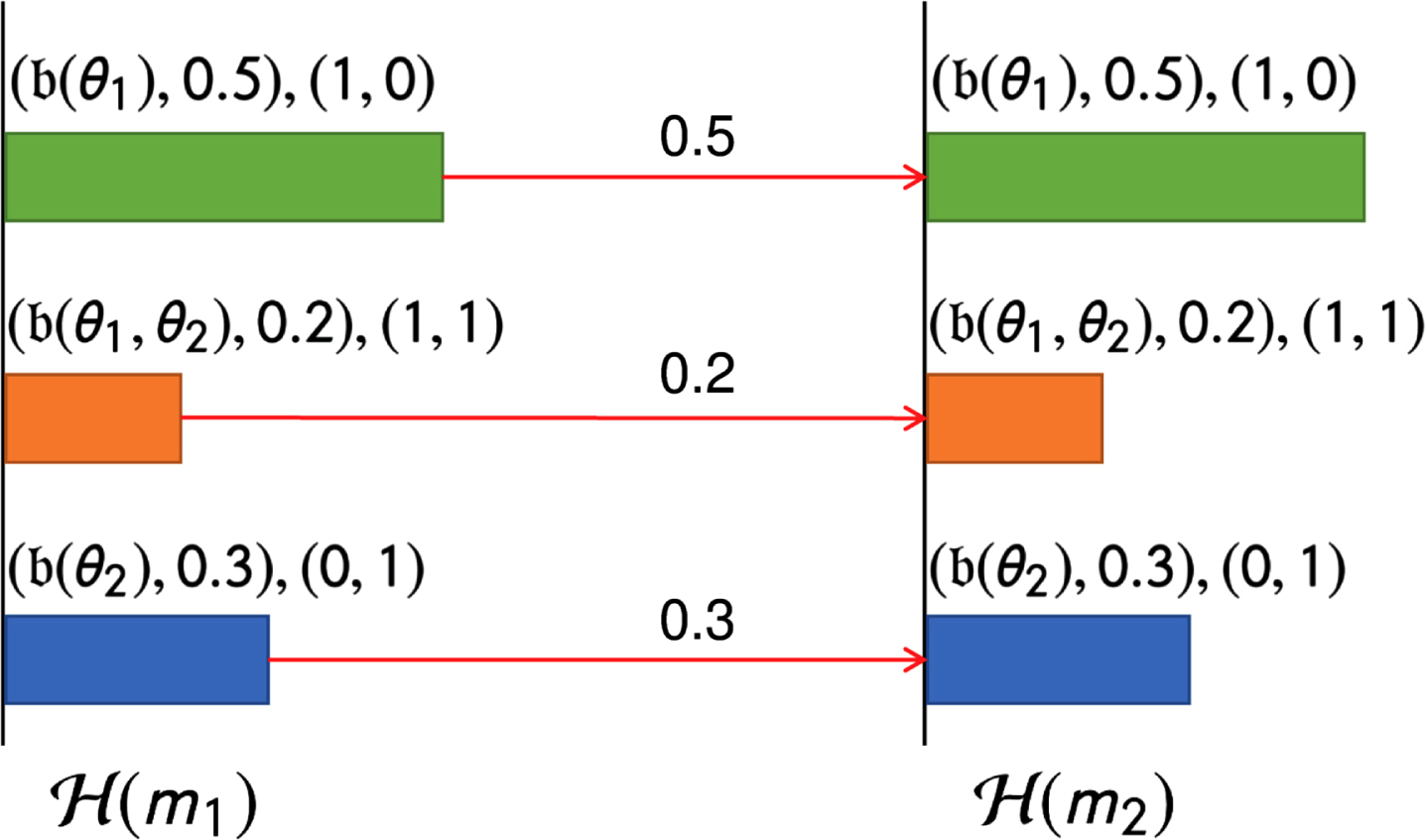
The corresponding locations of bins $b (θ_{1})$ , $b (θ_{2})$ , and $b (θ_{1}, θ_{2})$ are (1, 0), (0, 1), and (1, 1). To compute the BMD between m₁ and m₂, we must to minimize the total cost for moving beliefs from $H (m_{1})$ to $H (m_{2})$ . As shown in Fig. 1, transferring all belief in one bin in $H (m_{1})$ to the equivalent bin in $H (m_{2})$ can minimize the total cost. Accordingly, BMD (m₁, m₂) is computed as follows: $\begin{matrix} BMD (m_{1}, m_{2}) & = 0.5 \times δ (θ_{1}, θ_{1}) + 0.3 \times δ (θ_{2}, θ_{2}) \\ + 0.2 \times δ ((θ_{1}, θ_{2}), (θ_{1}, θ_{2})) \\ = 0.5 \times 0 + 0.3 \times 0 + 0.2 \times 0 = 0 . \end{matrix}$

Fig. 1

An example to show the computation of BMD between m₁ and m₂. m₁ and m₂ have the same probability assignment, and thus the mapped histograms are identical. To minimize the total cost for moving beliefs from $H (m_{1})$ to $H (m_{2})$ , we can transfer all belief in a bin in $H (m_{1})$ to the equivalent bin in $H (m_{2})$ . The BMD is 0.

Example 5 shows us that when two BPAs have the same probability assignment, their BMD is 0.

Example 6. Let Θ = {θ₁, θ₂} be an FoD, and m₁, m₂ be two BPAs. $\begin{matrix} m_{1} : & m_{1} ({θ_{1}}) = 0.5, m_{1} ({θ_{2}}) = 0.3, \\ m_{1} ({θ_{1}, θ_{2}}) = 0.2, \\ m_{2} : & m_{2} ({θ_{1}}) = 0.3, m_{2} ({θ_{2}}) = 0.2, \\ m_{2} ({θ_{1}, θ_{2}}) = 0.5 . \end{matrix}$ Here, m₁ and m₂ are not identical. The mapped histograms of m₁ and m₂ respectively are $\begin{matrix} H (m_{1}) = {(b (θ_{1}), 0.5), (b (θ_{2}), 0.3), (b (θ_{1}, θ_{2}), 0.2)}, \\ H (m_{2}) = {(b (θ_{1}), 0.3), (b (θ_{2}), 0.2), (b (θ_{1}, θ_{2}), 0.5)} . \end{matrix}$

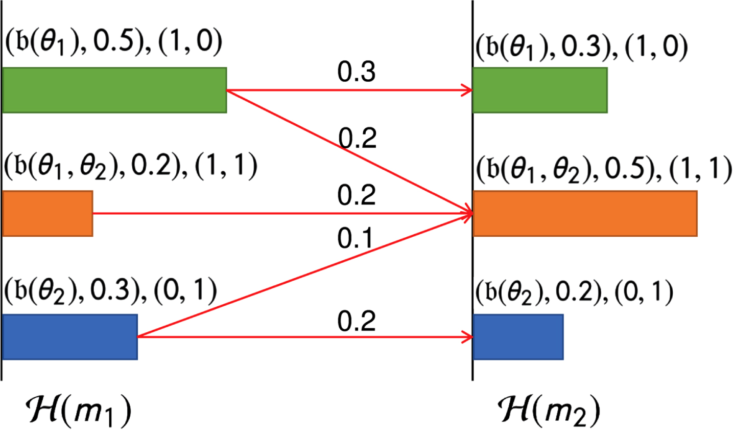
The corresponding locations of bins $b (θ_{1})$ , $b (θ_{2})$ , and $b (θ_{1}, θ_{2})$ are (1, 0), (0, 1), and (1, 1). Fig. 2 depicts the flow of beliefs that can minimize the total cost. Thus, the distance between m₁ and m₂ is calculated as follows: $\begin{matrix} BMD (m_{1}, m_{2}) \\ = 0.3 \times δ (θ_{1}, θ_{1}) + 0.2 \times δ (θ_{1}, (θ_{1}, θ_{2})) \\ + 0.2 \times δ ((θ_{1}, θ_{2}), (θ_{1}, θ_{2})) \\ + 0.2 \times δ (θ_{2}, θ_{2}) + 0.1 \times δ (θ_{2}, (θ_{1}, θ_{2})) \\ = 0.3 \times 0 + 0.2 \times 1 + 0.2 \times 0 \\ + 0.2 \times 0 + 0.1 \times 1 = 0.3 . \end{matrix}$

Fig. 2

Another example to show the computation of BMD between m₁ and m₂. m₁ and m₂ have different probability assignment, and thus the mapped histograms are not identical. In this example, the belief in a bin in $H (m_{1})$ can be moved to different bins in $H (m_{2})$ . The flow of beliefs in this figure can minimize the total cost. The BMD is 0.3.

Example 7. Let Θ = {θ₁, θ₂, θ₃} be an FoD, and m₁, m₂ and m₃ be three BPAs. $\begin{matrix} m_{1} : & m_{1} ({θ_{1}}) = 0.58, m_{1} ({θ_{2}}) = 0.07, \\ m_{1} ({θ_{1}, θ_{3}}) = 0.35, \\ m_{2} : & m_{2} ({θ_{1}}) = 0.51, m_{2} ({θ_{2}}) = 0.19, \\ m_{2} ({θ_{1}, θ_{3}}) = 0.3, \\ m_{3} : & m_{3} ({θ_{1}}) = 0, m_{3} ({θ_{2}}) = 0.9, \\ m_{3} ({θ_{1}, θ_{2}, θ_{3}}) = 0.1 . \end{matrix}$ It is apparent that m₁ is similar with m₂ but conflicts with m₃. The mapped histograms of these three BPAs are

$\begin{matrix} H (m_{1}) = {(b (θ_{1}), 0.58), (b (θ_{2}), 0.07), (b (θ_{1}, θ_{3}), 0.35)}, \\ H (m_{2}) = {(b (θ_{1}), 0.51), (b (θ_{2}), 0.19), (b (θ_{1}, θ_{3}), 0.3)}, \\ H (m_{3}) = {(b (θ_{1}), 0), (b (θ_{2}), 0.9), (b (θ_{1}, θ_{2}, θ_{3}), 0.1)} . \end{matrix}$

The corresponding locations of bins $b (θ_{1})$ , $b (θ_{2})$ , $b (θ_{1}, θ_{3})$ and $b (θ_{1}, θ_{2}, θ_{3})$ are (1, 0, 0), (0, 1, 0), (1, 0, 1) and (1, 1, 1). Figure 3 shows the optimal flow of beliefs from one histogram to another. Take Fig. 3(a) as an example, this figure presents the optimal flow of beliefs from $H (m_{1})$ to $H (m_{2})$ . Therefore, the distance between m₁ and m₂ is computed as follows: $\begin{matrix} BMD (m_{1}, m_{2}) \\ = 0.51 \times δ (θ_{1}, θ_{1}) + 0.07 \times δ (θ_{2}, θ_{2}) \\ + 0.3 \times δ ((θ_{1}, θ_{3}), (θ_{1}, θ_{3})) \\ + 0.07 \times δ (θ_{1}, θ_{2}) + 0.05 \times δ ((θ_{1}, θ_{3}), θ_{2}) \\ = 0.51 \times 0 + 0.07 \times 0 + 0.3 \times 0 \\ + 0.07 \times \sqrt{2} + 0.05 \times \sqrt{3} = 0.1856 . \end{matrix}$

Fig. 3

The optimal flow of beliefs between different histograms in Example 7.

Analogously, we can calculate the two other distances according to Figs. 3(a) and (b), which are BMD (m₁, m₃) =1.3533 and BMD (m₂, m₃) =1.1677. Clearly, m₁ is close to m₂ but far away from m₃. Likewise, m₂ is close to m₁ but far away from m₃. The results indicate that BMD can measure the consistency relationship between BPAs.

Example 8. Let m₁, m₂ be two BPAs defined on FoD Θ = {θ₁, θ₂}, which are $\begin{matrix} m_{1} : m_{1} ({θ_{1}}) = α, m_{1} ({θ_{1}, θ_{2}}) = 1 - α, \\ m_{2} : m_{2} ({θ_{1}}) = 0.8, m_{2} ({θ_{2}}) = 0.2, \end{matrix}$ here, α ∈ [0, 1]. The BMD between m₁ and m₂ with different values of α is depicted in Fig. 4.

Fig. 4

An example to show the distance between m₁ and m₂ with the change of α.

In Example 8, m₂ gives high belief to θ₁, which is m₂ ({θ₁}) =0.8. As the value of parameter α increases from 0 to 1, the support degree of m₁ to θ₁ is gradually enhanced. According to the definition of BMD, the distance between m₁ and m₂, when α is in [0, 0.8], can be calculated as follows: $\begin{matrix} BMD (m_{1}, m_{2}) \\ = α \times δ (θ_{1}, θ_{1}) + 0.2 \times δ ((θ_{1}, θ_{2}), θ_{2}) \\ + (0.8 - α) \times δ ((θ_{1}, θ_{2}), θ_{1}) \\ = α \times 0 + 0.2 \times 1 + (0.8 - α) \times 1 \\ = 1 - α . \end{matrix}$ When α is in (0.8, 1], the distance is measured as follows: $\begin{matrix} BMD (m_{1}, m_{2}) \\ = 0.8 \times δ (θ_{1}, θ_{1}) + (1 - α) \times δ ((θ_{1}, θ_{2}), θ_{2}) \\ + (α - 0.8) \times δ (θ_{1}, θ_{2}) \\ = 0.8 \times 0 + (1 - α) \times 1 + (α - 0.8) \times \sqrt{2} \\ = 1 - α + (α - 0.8) \times \sqrt{2} . \end{matrix}$

As shown in Fig. 4, with the increasing of α from 0 to 0.8, the distance between m₁ and m₂ is decreasing. When α = 0.8, the distance is the smallest. Whereas, when α changes from 0.8 to 1, the distance is increasing. The reason is the support degree of m₁ to θ₁ is gradually higher than that of m₂ to θ₁.

Example 9. Further, we use an example presented in [44] to analyze the performance of the proposed BMD metric. Suppose there is an FoD with 20 elements, i.e., Θ = {θ₁, θ₂, ⋯ , θ₂₀}, two BPAs are defined as $\begin{matrix} m_{1} : & m_{1} ({θ_{1}, θ_{2}, θ_{3}}) = 0.05, m_{1} ({θ_{7}}) = 0.05, \\ m_{1} (A) = 0.8, m_{1} (Θ) = 0.1, \\ m_{2} : & m_{2} ({θ_{1}, θ_{2}, \dots, θ_{5}}) = 1 . \end{matrix}$ A is a variable set. As A changes, the distances between m₁ and m₂ measured by BMD is shown in Fig. 5.

Fig. 5

The BMDs between m₁ and m₂ vary with the size of A.

In Fig. 5, size of A equals to l (1 < l < 20) means that A = {θ₁, θ₂, ⋯ , θ_l}. From this figure, one can see that the proposed BMD metric is reasonable to measure the difference between BPAs that contain multi-focal elements. The trend of the distance between m₁ and m₂ with A changes is very obvious. When A changes from {θ₁} to {θ₁, θ₂, ⋯ , θ₅}, the distance gradually decreases. When A equals to {θ₁, θ₂, ⋯ , θ₅}, the distance is the minimum because the amount of belief transferred cross-bin is the minimum. When A changes from {θ₁, θ₂, ⋯ , θ₅} to {θ₁, θ₂, ⋯ , θ₂₀}, the distance gradually increases since the cost that must be paid to transfer belief from $H (m_{1})$ to $H (m_{2})$ gradually increases.

4 The proposed method

In this section, a new combination method is designed to fuse evidence with their distances measured by the proposed Belief Mover’s Distance. The new method computes the weight of a piece of evidence from two aspects. The first part of weight considers the support relationship between different pieces of evidence as in [14], and the second part takes the distance of this evidence from the negative ideal BPA into account. The final weight of the evidence is unified by combining both parts. Eventually, the weighted average evidence is obtained by calculating the weighted sum of multiple pieces of evidence and then fused via the Dempster’s combination rule. The flowchart of the proposed method is depicted in Fig. 6.

Fig. 6

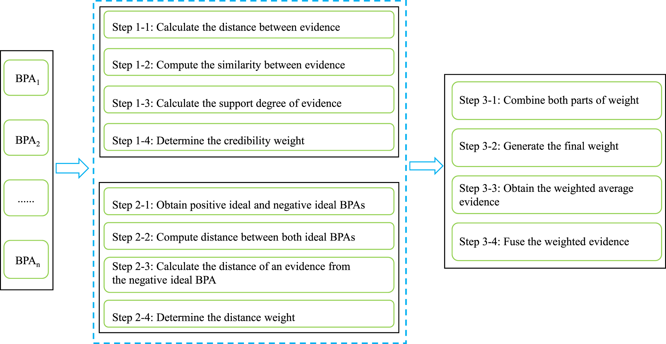
Flowchart of the proposed method.

In what follows, the detailed process of the proposed method will be elaborated.

4.1 Calculate the credibility weight

Step 1-1: Calculate the distance between bodies of evidence.

Suppose M = {m₁, m₂, ⋯ , m_n} is a set of BPAs defined on the FoD Θ. According to Definition 11, a distance matrix can be calculated as $\begin{matrix} D = [\begin{matrix} 0 & {BMD}_{12} & \dots & {BMD}_{1 n} \\ {BMD}_{21} & 0 & \dots & {BMD}_{2 n} \\ ⋮ & ⋮ & ⋱ & ⋮ \\ {BMD}_{n 1} & {BMD}_{n 2} & \dots & 0 \end{matrix}], \end{matrix}$ where BMD_ij is the BMD between m_i and m_j.

Step 1-2: Compute the similarity between bodies of evidence.

Here, we define the similarity between BPAs m_i and m_j as

${sim}_{ij} = e^{- {BMD}_{ij}} .$ (13)

Then, we get the similarity matrix as follows: $\begin{matrix} S = [\begin{matrix} 1 & {sim}_{12} & \dots & {sim}_{1 n} \\ {sim}_{21} & 1 & \dots & {sim}_{2 n} \\ ⋮ & ⋮ & ⋱ & ⋮ \\ {sim}_{n 1} & {sim}_{n 2} & \dots & 1 \end{matrix}] . \end{matrix}$

Step 1-3: Calculate the support degree of evidence.

If evidence m_i is similar with another one, namely m_j, we say that m_i is supported by m_j. Thence, the support degree of m_i is defined as

$\sup (m_{i}) = \sum_{j = 1, j \neq i}^{n} {sim}_{ij}, i = 1, 2, \dots, n .$ (14)

Step 1-4: Determine the credibility weight.

According to [14], if a piece of evidence has bigger support degree, then this evidence is more credible and consequently has higher weight when averaging multiple pieces of evidence. The credibility weight of a piece of evidence is determined in Eq. (15).

$w_{crd} (m_{i}) = \frac{\sup (m_{i})}{\sum_{j = 1}^{n} \sup (m_{j})}, i = 1, 2, \dots, n .$ (15)

4.2 Calculate the distance weight

Step 2-1: Obtain the positive ideal BPA and negative ideal BPA.

As per Definition 6, the positive ideal and negative ideal BPAs have the minimum and maximum of Deng entropy, respectively. As aforementioned, there are multiple positive ideal BPAs and one negative ideal BPA on FoD Θ. Suppose m⁺ is one positive ideal BPA and m^- is the negative ideal BPA, which can be computed according to the analysis in subsection 2.2.

Step 2-2: Compute the distance between the positive ideal BPA and negative ideal BPA.

Among all BPAs defined on FoD Θ, the positive ideal BPA and negative ideal one have the maximum distance, which is denoted as BMD_max, BMD_max = BMD (m⁺, m^-).

Step 2-3: Calculate the distance of a piece of evidence from the negative ideal BPA.

After computing the distance of each evidence from the negative ideal BPA, a distance vector $D^{-}$ is obtained, which is $D^{-} = {[{BMD}_{1}^{-}, {BMD}_{2}^{-}, \dots, {BMD}_{n}^{-}]}^{T},$ where ${BMD}_{i}^{-} = BMD (m_{i}, m^{-})$ .

Then, we normalize the distance vector $D^{-}$ by dividing its elements by BMD_max. The normalized distance vector is denoted as $X^{-} = {[x_{1}, x_{2}, \dots, x_{n}]}^{T},$ where $x_{i} = \frac{{BMD}_{i}^{-}}{{BMD}_{\max}}$ .

Step 2-4: Determine the distance weight.

In this step, we estimate the second part of weight of the evidence based on its distance from the negative ideal BPA. Before defining the distance weight of the evidence, we measure the importance of the evidence as

$I (m_{i}) = {\begin{matrix} x_{i}, & if x_{i} < = β \\ 1 - x_{i}, & otherwise \end{matrix}$ (16) where β is an adjustable parameter. The motivation for Eq. (16) comes from two aspects: (1) a valuable evidence should be far away from the negative ideal BPA; (2) a conflicting evidence is usually close to some positive ideal BPA. The definition of Eq. (16) can assign high importance to valuable evidence and suppress the importance of conflicting evidence. After a simple test, we set β = 0.75 in this work.

The distance weight of a piece of evidence is determined by Eq. (17).

$w_{dist} (m_{i}) = \frac{I (m_{i})}{\sum_{j = 1}^{n} I (m_{j})}, i = 1, 2, \dots, n .$ (17)

4.3 Generate and fuse the weighted average evidence

Step 3-1: Combine both parts of weight.

By combining the credibility weight and distance weight, the modified weight of each piece of evidence is computed as

$W (m_{i}) = w_{crd} (m_{i}) \times w_{dist} (m_{i}), i = 1, 2, \dots, n .$ (18)

Step 3-2: Generate the final weight.

The final weight is the normalized modified weight, which is defined as

$W^{*} (m_{i}) = \frac{W (m_{i})}{\sum_{j = 1}^{n} W (m_{j})}, i = 1, 2, \dots, n .$ (19) Clearly, $\sum_{i = 1}^{n} W^{*} (m_{i}) = 1$ .

Step 3-3: Obtain the weighted average evidence.

Using the final weight of each piece of evidence, the weighted average evidence, denoted as $M$ , is attained as

$M = \sum_{i = 1}^{n} W^{*} (m_{i}) \times m_{i} .$ (20)

Step 3-4: Fuse the weighted evidence.

For n pieces of evidence, the final combination result can be obtained by fusing the weighted average evidence $M$ by using the Dempster’s combination rule n - 1 times.

4.4 Illustrative example

We think it is helpful to show the process of the proposed method by providing an example. Here, we consider the three BPAs given in Example 7 again, which are $\begin{matrix} m_{1} : & m_{1} ({θ_{1}}) = 0.58, m_{1} ({θ_{2}}) = 0.07, \\ m_{1} ({θ_{1}, θ_{3}}) = 0.35, \\ m_{2} : & m_{2} ({θ_{1}}) = 0.51, m_{2} ({θ_{2}}) = 0.19, \\ m_{2} ({θ_{1}, θ_{3}}) = 0.3, \\ m_{3} : & m_{3} ({θ_{1}}) = 0.00, m_{3} ({θ_{2}}) = 0.90, \\ m_{3} ({θ_{1}, θ_{2}, θ_{3}}) = 0.1 . \end{matrix}$ Evidently, both m₁ and m₂ support θ₁ with more than 50% belief, and highly conflict with m₃, which assigns zero belief to θ₁. In what follows, the calculation is presented.

Firstly, calculate the credibility weight.

The BMDs among the three BPAs are $\begin{matrix} BMD (m_{1}, m_{2}) = 0.1856, \\ BMD (m_{1}, m_{3}) = 1.3533, \\ BMD (m_{2}, m_{3}) = 1.1677 . \end{matrix}$ According to Eq. (13), the similarity matrix is obtained as $\begin{matrix} S = [\begin{matrix} 1 & 0.8306 & 0.2584 \\ 0.8306 & 1 & 0.3111 \\ 0.2584 & 0.3111 & 1 \end{matrix}] . \end{matrix}$

Then, using Eqs. (14) and (15), the support degrees and credibility weights of these pieces of evidence are computed. The support degrees are sup (m₁) =1.0890, sup (m₂) =1.1417, and sup (m₃) =0.5695; the credibility weights are w_crd (m₁) =0.3889, w_crd (m₂) =0.4077, and w_crd (m₃) =0.2034.

Secondly, compute the distance weight.

Let m⁺, m^- denote the positive ideal BPA and negative ideal BPA on Θ = {θ₁, θ₂, θ₃}, which are defined as $\begin{matrix} m^{+} ({θ_{1}}) = 1, \\ m^{-} ({θ_{1}}) = m^{-} ({θ_{2}}) = m^{-} ({θ_{3}}) = \frac{1}{19}, \\ m^{-} ({θ_{1}, θ_{2}}) = m^{-} ({θ_{1}, θ_{3}}) = m^{-} ({θ_{2}, θ_{3}}) = \frac{3}{19}, \\ m^{-} ({θ_{1}, θ_{2}, θ_{3}}) = \frac{7}{19} . \end{matrix}$ As mentioned above, BMD_max = BMD (m⁺, m^-) =1.2592.

Next, we compute the distances of three BPAs from m^-, and then normalize these distances. The obtained distance vector and normalized distance vector are $D^{-} = [0.9345, 0.8674, 1.1177]^{T}$ and $X^{-} = {[0.7422, 0.6889, 0.8877]}^{T}$ , respectively. Then, according to Eq. (16), we attain I (m₁) =0.7422, I (m₂) =0.6889, and I (m₃) =0.1123; according to Eq. (17), we get w_dist (m₁) =0.4809, w_dist (m₂) =0.4463, and w_dist (m₃) =0.0728.

Finally, obtain the fused result.

Based on Eqs. (18) and (19), we compute the modified and final weights of three BPAs. The modified weights are W (m₁) =0.1870, W (m₂) =0.1920, and W (m₃) =0.0148, while the final weights are $W^{*} (m_{1}) = 0.4873$ , $W^{*} (m_{2}) = 0.4742$ , and $W^{*} (m_{3}) = 0.0386$ . Then, by using Eq. (20), the weighted average evidence $M$ is computed as $\begin{matrix} M ({θ_{1}}) = 0.5244, M ({θ_{2}}) = 0.1589, \\ M ({θ_{1}, θ_{3}}) = 0.3128, M ({θ_{1}, θ_{2}, θ_{3}}) = 0.0039 . \end{matrix}$

To attain the final result, $M^{*}$ , we combine $M$ by means of Dempster’s rule 2 times. The result is $\begin{matrix} M^{*} ({θ_{1}}) = 0.9398, \\ M^{*} ({θ_{2}}) = 0.0072, \\ M^{*} ({θ_{1}, θ_{3}}) = 0.0530 . \end{matrix}$ By applying the pignistic probability transformation, we get $\begin{matrix} {BetP}_{M^{*}} ({θ_{1}}) = 0.9663, \\ {BetP}_{M^{*}} ({θ_{2}}) = 0.0072, \\ {BetP}_{M^{*}} ({θ_{3}}) = 0.0265 . \end{matrix}$

These results indicate that the proposed method can reduce the negative effect caused by m₃ and assign high belief to hypothesis θ₁. For the purpose of comparison, Table 1 lists the fusion results of several baseline methods and Fig. 7 depicts the corresponding pignistic probability. Both Table 1 and Fig. 7 show that the proposed method gives higher belief and pignistic probability to hypothesis θ₁ than others. As a result, the proposed method is more effective than others for the illustrative example which contains highly conflicting evidence.

Table 1
Fusion results of different methods for the illustrative example

Method {θ₁} {θ₂} {θ₁, θ₃} Θ

Dempster’s 0.7315 0.1501 0.1185 0

Murphy’s 0.7058 0.2430 0.0511 1.22E-04

Deng et al. ’s 0.8889 0.0558 0.0553 1.30E-05

Wang and Xiao’s 0.9144 0.0310 0.0546 4.12E-06

Zhang and Deng’s 0.5224 0.4353 0.042 2.58E-04

Yang et al. ’s 0.8296 0.1153 0.055 4.24E-05

Lin et al. ’s 0.8063 0.1394 0.0543 5.35E-05

Xia et al. ’s 0.6231 0.3291 0.0476 1.86E-04

Yu et al. ’s 0.7890 0.0528 0.1582 0

The proposed 0.9398 0.0072 0.0530 0

Method	{θ₁}	{θ₂}	{θ₁, θ₃}	Θ
Dempster’s	0.7315	0.1501	0.1185	0
Murphy’s	0.7058	0.2430	0.0511	1.22E-04
Deng et al. ’s	0.8889	0.0558	0.0553	1.30E-05
Wang and Xiao’s	0.9144	0.0310	0.0546	4.12E-06
Zhang and Deng’s	0.5224	0.4353	0.042	2.58E-04
Yang et al. ’s	0.8296	0.1153	0.055	4.24E-05
Lin et al. ’s	0.8063	0.1394	0.0543	5.35E-05
Xia et al. ’s	0.6231	0.3291	0.0476	1.86E-04
Yu et al. ’s	0.7890	0.0528	0.1582	0
The proposed	0.9398	0.0072	0.0530	0

5 Experiment

To further show the superior performance of the proposed method, a numerical example and two applications in fault diagnosis and classification problem are demonstrated in this section. The compared methods include Dempster’s combination rule [1], Murphy’s method [10], Deng et al. ’s method [14], Wang and Xiao’s method [25], Zhang and Deng’s method [7], Yang et al. ’s method [22], Lin et al. ’s method [24], Xia et al. ’s method [27], and Yu et al. ’s method [16].

5.1 Numerical example

Here, we employ the fictitious example used in [7]. Suppose there are three objects, namely A, B, and C, in a multi-sensor-based target recognition system [7]. Thence, the FoD is Θ = {A, B, C}. Based the results reported by five different sensors, five pieces of evidence are derived, which are outlined in Table 2. Assume hypothesis C is the true target. From Table 2, it can be seen that m₂ is abnormal because it highly conflicts with others.

Table 2
Five pieces of evidence collected from different sensors [7]

BPA {A} {B} {C} Θ

m ₁ 0.1 0.2 0.3 0.4

m ₂ 0.2 0.8 0.0 0.0

m ₃ 0.1 0.1 0.6 0.2

m ₄ 0.1 0.1 0.7 0.1

m ₅ 0.1 0.1 0.7 0.1

BPA	{A}	{B}	{C}	Θ
m ₁	0.1	0.2	0.3	0.4
m ₂	0.2	0.8	0.0	0.0
m ₃	0.1	0.1	0.6	0.2
m ₄	0.1	0.1	0.7	0.1
m ₅	0.1	0.1	0.7	0.1

Table 3 lists the combination results of the proposed method and nine compared ones. From Table 3, we can observe that Dempster’s rule generates the counter-intuitive conclusion that object B has the highest support, because it is disturbed by m₂. Whereas, all other methods recognize the true target C. In addition, in comparison with other methods, the proposed one has a faster convergence rate and the highest belief to the correct target. Because m₂ is abnormal and gives high support to B, most of the methods, except Wang and Xiao’s method [25] and the proposed method, wrongly support target B when only combining m₁ and m₂. However, after combining m₁, m₂ and m₃, the proposed method already can identify the true target C with belief = 0.7130. When combining m₁, m₂, m₃ and m₄, the proposed method assigns near 94% belief to object C. In other words, the proposed method has a very high probability of detecting the true target even if combining partial sources of evidence. Furthermore, Table 4 outlines the pignistic probability of object C generated by different methods with incremental evidence. As observed from Table 4, the proposed method has a higher speed in convergence and higher support to true target than others. In a nutshell, our method is more effective when handling conflicting evidence.

Table 3

Fusion results of different methods for numerical example

Method	belief	m ₁₂	m _1-3	m _1-4	m _1-5
Dempster’s	m ({A})	0.1724	0.1724	0.1724	0.1724
	m ({B})	0.8276	0.8276	0.8276	0.8276
Murphy’s	m ({A})	0.1260	0.0885	0.0430	0.0152
	m ({B})	0.6870	0.5304	0.3002	0.1221
	m ({C})	0.1260	0.3567	0.6511	0.8617
	m (Θ)	0.0611	0.0244	0.0056	0.0010
Deng et al. ’s	m ({A})	0.1260	0.0911	0.0375	0.0103
	m ({B})	0.6870	0.4340	0.1633	0.0420
	m ({C})	0.1260	0.4421	0.7922	0.9467
	m (Θ)	0.0611	0.0329	0.0069	0.0009
Wang and Xiao’s	m ({A})	0.1279	0.0891	0.0424	0.0145
	m ({B})	0.4275	0.2524	0.1161	0.0392
	m ({C})	0.2994	0.6033	0.8281	0.9439
	m (Θ)	0.1452	0.0552	0.0134	0.0024
Zhang and Deng’s	m ({A})	0.1012	0.0771	0.0285	0.0079
	m ({B})	0.8516	0.4585	0.1476	0.0388
	m ({C})	0.0318	0.4481	0.8204	0.9528
	m (Θ)	0.0154	0.0164	0.0034	0.0005
Yang et al. ’s	m ({A})	0.1260	0.0895	0.0392	0.0125
	m ({B})	0.6870	0.4413	0.2044	0.0694
	m ({C})	0.1260	0.4390	0.7501	0.9171
	m (Θ)	0.0611	0.0302	0.0063	0.0010
Lin et al. ’s	m ({A})	0.1260	0.0912	0.0409	0.0122
	m ({B})	0.6870	0.4662	0.2063	0.0608
	m ({C})	0.1260	0.4118	0.7458	0.9260
	m (Θ)	0.0611	0.0308	0.0070	0.0011
Xia et al. ’s	m ({A})	0.1189	0.0828	0.0389	0.0130
	m ({B})	0.7579	0.6001	0.3331	0.1281
	m ({C})	0.0830	0.3000	0.6243	0.8583
	m (Θ)	0.0402	0.0171	0.0037	0.0006
Yu et al. ’s	m ({A})	0.1724	0.1132	0.0565	0.0168
	m ({B})	0.8276	0.2960	0.1014	0.0255
	m ({C})	0.0000	0.4755	0.8173	0.9551
	m (Θ)	0.0000	0.1153	0.0248	0.0025
The proposed	m ({A})	0.1303	0.0719	0.0190	0.0043
	m ({B})	0.5005	0.1779	0.0380	0.0077
	m ({C})	0.2486	0.7130	0.9391	0.9877
	m (Θ)	0.1206	0.0372	0.0039	0.0004

Table 4

Pignistic probability of object C with incremental evidence

Method	m ₁₂	m _1-3	m _1-4	m _1-5
Dempster’s	0	0	0	0
Murphy’s	0.1463	0.3648	0.6530	0.8620
Deng et al. ’s	0.1463	0.453	0.7945	0.9470
Wang and Xiao’s	0.3478	0.6217	0.8325	0.9447
Zhang and Deng’s	0.0369	0.4535	0.8216	0.9530
Yang et al. ’s	0.1463	0.4491	0.7522	0.9174
Lin et al. ’s	0.1463	0.4220	0.7482	0.9263
Xia et al. ’s	0.0964	0.3057	0.6255	0.8585
Yu et al. ’s	0	0.5139	0.8256	0.9560
The proposed	0.2888	0.7253	0.9404	0.9878

The reason is that our method takes into account two aspects of weight, which makes full use of the new Belief Mover’s Distance. Thence, it increases the weights of reliable evidence whilst decreases the weights of unreliable evidence.

5.2 Application in fault diagnosis

In this experiment, a case study in fault diagnosis of a rotating machinery system [24,25, 24,25] is adopted to evaluate the effectiveness of our proposed method.

A rotating machinery system has four different fault types: “Imbalance”, “Shaft crack”, “Misalignment”, and “Bearing loose”, which are symbolically marked as F₁, F₂, F₃, and F₄. So, the FoD is Θ = {F₁, F₂, F₃, F₄}. Five sensors are distributed in the system to monitor its status. When working, these sensors can continuously report diagnostic evidence for different faults. At some time, the fault F₃ happened, and then five sensors got a lot of data. According to the data reported by these sensors, BPAs are calculated, which are listed in Table 5. In Table 5, m₁, m₂, and m₄ suggest the fault is F₃. However, m₃ says the fault is F₂, and m₅ believes the fault is F₄.

Table 5
Five BPAs calculated from five sensors [24, 25]

BPA {F₁} {F₂} {F₃} {F₄}

m ₁ 0.1469 0.2057 0.4660 0.1813

m ₂ 0.1521 0.1935 0.4631 0.1914

m ₃ 0.1278 0.5008 0.2221 0.1493

m ₄ 0.1459 0.2396 0.4395 0.1750

m ₅ 0.2068 0.1399 0.1755 0.4777

BPA	{F₁}	{F₂}	{F₃}	{F₄}
m ₁	0.1469	0.2057	0.4660	0.1813
m ₂	0.1521	0.1935	0.4631	0.1914
m ₃	0.1278	0.5008	0.2221	0.1493
m ₄	0.1459	0.2396	0.4395	0.1750
m ₅	0.2068	0.1399	0.1755	0.4777

Table 6 presents the fusion results of ten methods. Based on the results in Table 6, all methods can recognize the true fault F₃. Notably, the proposed method gives the highest support to F₃. In addition, the support degree of F₃ decreases when m₁, m₂ and m₃ are fused owning to conflicting information from m₃. Similar phenomenon also appears when all BPAs are combined, because the fifth sensor does not support F₃. Nonetheless, the corresponding drop of the proposed method is the slightest. It indicates that the proposed method suffers less negative effects from conflicting evidence.

Table 6

Fusion results of different methods for fault diagnosis

Method	belief	m _1,2	m _1-3	m _1-4	m _1-5
Dempster’s	m ({F₁})	0.0715	0.0376	0.0153	0.0176
	m ({F₂})	0.1273	0.2626	0.1758	0.1367
	m ({F₃})	0.6902	0.6315	0.7755	0.7565
	m ({F₄})	0.1110	0.0683	0.0334	0.0886
Murphy’s	m ({F₁})	0.0715	0.0314	0.0128	0.0124
	m ({F₂})	0.1274	0.2946	0.2000	0.1472
	m ({F₃})	0.6901	0.6165	0.7593	0.7380
	m ({F₄})	0.1110	0.0575	0.0280	0.0960
Deng et al. ’s	m ({F₁})	0.0715	0.0315	0.0125	0.0108
	m ({F₂})	0.1274	0.2602	0.1671	0.1244
	m ({F₃})	0.6901	0.6504	0.7926	0.7845
	m ({F₄})	0.1110	0.0580	0.0277	0.0753
Wang and Xiao’s	m ({F₁})	0.0715	0.0315	0.0125	0.0107
	m ({F₂})	0.1274	0.2600	0.1632	0.1200
	m ({F₃})	0.6901	0.6505	0.7967	0.7901
	m ({F₄})	0.1111	0.0580	0.0276	0.0743
Zhang and Deng’s	m ({F₁})	0.0729	0.0309	0.0128	0.0152
	m ({F₂})	0.1238	0.3712	0.2330	0.1511
	m ({F₃})	0.6894	0.5422	0.7265	0.6781
	m ({F₄})	0.1143	0.0557	0.0277	0.1467
Yang et al. ’	m ({F₁})	0.0715	0.0314	0.0128	0.0122
	m ({F₂})	0.1274	0.2943	0.1996	0.1472
	m ({F₃})	0.6901	0.6168	0.7596	0.7406
	m ({F₄})	0.1110	0.0575	0.0280	0.0938
Lin et al. ’s	m ({F₁})	0.0715	0.0315	0.0125	0.0108
	m ({F₂})	0.1274	0.2675	0.1692	0.1252
	m ({F₃})	0.6901	0.6431	0.7906	0.7834
	m ({F₄})	0.1110	0.0579	0.0276	0.0755
Xia et al. ’s	m ({F₁})	0.0715	0.0314	0.0128	0.0125
	m ({F₂})	0.1274	0.3000	0.2054	0.1517
	m ({F₃})	0.6901	0.6113	0.7538	0.7320
	m ({F₄})	0.1110	0.0574	0.0280	0.0974
Yu et al. ’s	m ({F₁})	0.0715	0.0546	0.0228	0.0233
	m ({F₂})	0.1273	0.2024	0.1321	0.1196
	m ({F₃})	0.6902	0.6536	0.8006	0.7819
	m ({F₄})	0.1110	0.0894	0.0445	0.0749
The proposed	m ({F₁})	0.0715	0.0315	0.0125	0.0102
	m ({F₂})	0.1274	0.2497	0.1583	0.1185
	m ({F₃})	0.6901	0.6607	0.8017	0.7988
	m ({F₄})	0.1110	0.0581	0.0275	0.0678

Moreover, the belief entropy of the final BPA fused by each method is shown in Fig. 8. From Fig. 8, the belief entropy of the final BPA calculated by the proposed method is the smallest, which indicates that the result produced by the proposed method has the smallest uncertain. As a consequence, the proposed method is flexible and effective in combination of evidence.

Fig. 7

Pignistic probability of hypothesis θ₁ computed by different methods for illustrative example.

Fig. 8

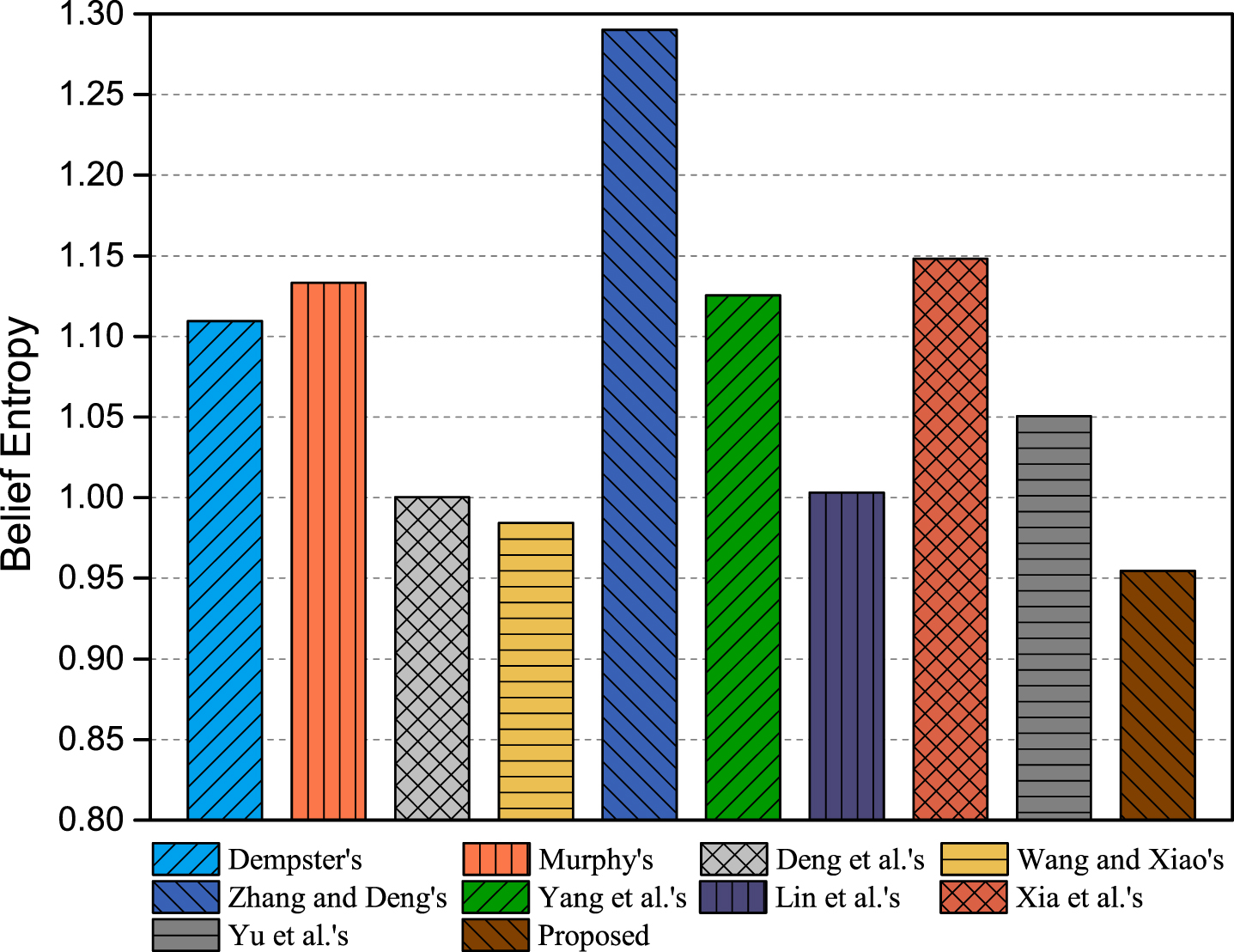
Belief entropy of the final BPA generated by each combination method.

5.3 Application in classification problem

In this subsection, another experiment on the Iris dataset is performed to verify the performance of the proposed method. The dataset covers three species of iris flowers, i.e., Setosa (Se), Versicolor (Ve) and Virginica (Vi), with four attributes, i.e., sepal length (SL), sepal width (SW), petal length (PL), and petal width (PW). Therefore, the FoD is Θ = {Se, Ve, Vi}. One species contains 50 instances in the dataset. In this experiment, we follow the experimental settings in [45], where 40 instances are randomly selected for a species to generate BPAs by using the interval number model. For a randomly chosen testing instance from Setosa, i.e., (4.5, 2.3, 1.3, 0.3), the BPA of each attribute generated based on the interval number model is listed in Table 7.

Table 7
BPAs of four attributes for an instance in Iris dataset [45]

Attribute {Se} {Ve} {Vi} {Se, Ve} {Se, Vi} {Ve, Vi} Θ

SL 0.200 0.104 0.081 0.170 0.170 0.104 0.170

SW 0.094 0.171 0.128 0.159 0.125 0.164 0.159

PL 0.710 0.118 0.076 0 0 0.096 0

PW 0.585 0.163 0.110 0 0 0.142 0

Attribute	{Se}	{Ve}	{Vi}	{Se, Ve}	{Se, Vi}	{Ve, Vi}	Θ
SL	0.200	0.104	0.081	0.170	0.170	0.104	0.170
SW	0.094	0.171	0.128	0.159	0.125	0.164	0.159
PL	0.710	0.118	0.076	0	0	0.096	0
PW	0.585	0.163	0.110	0	0	0.142	0

Table 7 manifests that attributes PL and PW give high belief to species Se, while attributes SL and SW assign small belief to all species. As a consequence, there is no clear conflict between these pieces of evidence. To determine the category of the testing instance, the four pieces of evidence are fused. The results of different methods are shown in Table 8. From this table, one can see that all methods can identify that the testing instance is likely to be Setosa with a belief of more than 60%, which conforms to the actual situation. Remarkably, the proposed method gives the highest belief to {Se}, which suggests that our method is more powerful than the compared ones in detecting the species of iris flowers. The Dempster’s rule correctly recognizes the category of the instance with the belief of 0.8137 since these pieces of evidence are reliable and not conflicting. However, Zhang and Deng’s method assigns only 60.17% belief to {Se}, which is much lower than those of other methods. Therefore, the method may be insufficient to combining evidence with no evident conflict.

Table 8

Fusion results of different methods for the Iris classification experiment

Method	{Se}	{Ve}	{Vi}	{Se, Ve}	{Se, Vi}	{Ve, Vi}	Θ
Dempster’s	0.8137	0.1138	0.0611	0	0	0.0062	0
Murphy’s	0.7492	0.1463	0.0865	0.0032	0.0025	0.0086	0.0002
Deng et al. ’s	0.7505	0.1453	0.0862	0.0031	0.0025	0.0085	0.0002
Wang and Xiao’s	0.6017	0.2208	0.1399	0.0105	0.0084	0.0136	0.0007
Zhang and Deng’s	0.8216	0.1078	0.0599	0.0011	0.0008	0.0061	0.0001
Yang et al. ’s	0.8210	0.1078	0.0603	0.0011	0.0009	0.0061	0.0001
Lin et al. ’s	0.7490	0.1462	0.0867	0.0032	0.0025	0.0086	0.0002
Xia et al. ’s	0.8270	0.1037	0.0584	0.0011	0.0009	0.0059	0.0001
Yu et al. ’s	0.7814	0.1286	0.0741	0	0	0.0115	0
The proposed	0.8799	0.0741	0.0393	0.0003	0.0002	0.0040	0

6 Discussion

In BMD, we employ the Euclidean distance as the ground distance, i.e., proposition distance. Actually, other distance measures, such as Manhattan distance and Jaccard coefficient, may also be used in our BMD. But, the influence of these measures to BMD should be further investigated. In addition, a side effect caused by Euclidean distance is the range of BMD is not in [0, 1]. Although this limitation does not affect the use of BMD in the proposed method, it may be not clear how different two BPAs are.

When gauging the distance weight of a piece of evidence, a parameter β is introduced in the proposed method. By using β, we intend to assign large weights to valuable evidence but suppress the importance of conflicting evidence. In this work, we just fix the value of β after a simple test. However, an ideal scenario is to automatically determine the value of β based on the information of evidence. In fact, this is a hard job that requires in-depth study.

The computation of BMD is to resolve the transportation problem. As a result, it may be time-consuming when the FoD contains more elements. Fortunately, some efforts have been made by researchers [30 , 37] to accelerate the computation of EMD. In this paper, we use the implementation of Ofir Pele and Michael Werman 1 .

7 Conclusion

In this paper, a new evidence combination method is proposed to address the issue of counter-intuitive results derived from highly conflicting evidence. In our proposed method, the Belief Mover’s Distance is introduced to accurately evaluate the differences among pieces of evidence. According to distances of evidence, the credibility weight and distance weight of each evidence are computed. Next, the final weight is calculated by unifying two aspects of weight, and then the weighted average evidence is produced by computing the weighted sum of all pieces of evidence. Finally, the weighted average evidence is fused via the classical Dempster’s combination rule. To demonstrate the superiority of the proposed method, a number of examples and applications are analyzed. The results show that the proposed method has faster convergence rate and higher effectiveness in comparison with others.

In the future work, we intend to study how to automatically set the value of parameter β in the proposed method according to the information of evidence. β is a critical parameter, the value of which can gravely affect the performance of the proposed method. In addition, we would like to further investigate the measure of proposition distance to make the range of BMD between 0 and 1. Specially, we want to apply our method to some real-environment applications, such as multiple sensor surveillance systems, complex network analysis, and pattern recognition.

Footnotes

Acknowledgments

We would like to thank Ofir Pele and Michael Werman for their implementation of the Earth Mover’s Distance, and the anonymous reviewers for their constructive comments to greatly improve the quality of this manuscript.

References

Dempster

A.P.

, Upper and lower probabilities induced by a multivalued mapping, The Annals of Mathematical Statistics 38(2) (1967), 325–339.

Shafer

, A Mathematical Theory of Evidence, Princeton University Press, Princeton, New Jersey, USA, 1976.

Yager

R.R.

, Uncertainty modeling using fuzzy measures, Knowledge-Based Systems 92 (2016), 1–8.

Denœux

, Decision-making with belief functions: A review, International Journal of Approximate Reasoning 109 (2019), 87–110.

Heendeni

J.N.

, Premaratne

, Murthi

M.N.

, Uscinski

and Scheutz

, A generalization of bayesian inference in the dempster-shafer belief theoretic framework, in: 2016 19th International Conference on Information Fusion (FUSION), 2016, pp. 798–804.

Xiao

, Multi-sensor data fusion based on the belief divergence measure of evidences and the belief, Information Fusion 46 (2019), 23–32.

Zhang

and Deng

, Combining conflicting evidence using the dematel method, Soft Computing 23(17) (2018), 8207–8216.

Dubois

, Liu

, Ma

and Prade

, The basic principles of uncertain An organised review of merging rules in different representation frameworks, Information Fusion 32(PartA) (2016), 12–39.

Zadeh

L.A.

, A simple view of the dempster-shafer theory of evidence and its implication for the rule of combination, AI Magazine 7(2) (1986), 85–90.

10.

Murphy

C.K.

, Combining belief functions when evidence conflicts, Decision Support Systems 29(1) (2000), 1–9.

11.

Liu

, Analyzing the degree of conflict among belief functions, Artificial Intelligence 170(11) (2006), 909–924.

12.

, Jiang

and Luo

, A flexible rule for evidential combination in Dempster–Shafer theory of evidence, Applied Soft Computing 85 (2019), 105512.

13.

Yager

R.R.

, Hedging in the combination of evidence, Journal of Information and Optimization Sciences 4(1) (1983), 73–81.

14.

Deng

, Shi

, Zhu

and Liu

, Combining belief functions based on distance of evidence, Decision Support Systems 38(3) (2004), 489–493.

15.

Smets

, Analyzing the combination of conflicting belief functions, Information Fusion 8(4) (2007), 387–412.

16.

, Yang

, Ma

and Min

, An improved conflicting evidence combination approach based on a new supporting probability distance, Expert Systems With Applications 42(12) (2015), 5139–5149.

17.

Wang

and Xiao

, An improved multi-source data fusion method based on the beliefand divergence measure, Entropy 21(6) (2019).

18.

Smets

, The combination of evidence in the transferable belief model, IEEE Transactions on Pattern Analysis and Machine Intelligence 12(5) (1990), 447–458.

19.

Dubois

and Prade

, Representation and combination of uncertainty with belief functions and possibility measures, Computational Intelligence 4(3) (1988), 244–264.

20.

Lefevre

, Colot

and Vannoorenberghe

, Belief function combination and conflict management, Information Fusion 3(2) (2002), 149–162.

21.

Jousselme

A.-L.

, Grenier

and Boss{é

{É.

, A new distance between two bodies of evidence, Information Fusion 2(2) (2001), 91–101.

22.

Yang

, Zhou

, Han

and Ai

, Weighted Evidence Combination with Ranking Distance, in: 2018 International Conference on Control, Automation and Information Sciences (ICCAIS), IEEE, 2018, pp. 61–66.

23.

Zhang

, Liu

, Chen

and Zhang

, Novel algorithm for identifying and fusing conflicting data in wireless sensor networks, Sensors 14(6) (2014), 9562–9581.

24.

Lin

, Li

, Yin

and Dou

, Multisensor fault diagnosis modeling based on the evidence theory, IEEE Transactions on Reliability 67(2) (2018), 513–521.

25.

Wang

and Xiao

, An improved multisensor data fusion method and its application in fault diagnosis, IEEE Access 7 (2019), 3928–3937.

26.

Deng

, Deng Entropy, Chaos,&, Fractals 91 (2016), 549–553.

27.

Xia

, Feng

, Liu

and Fei

, An evidential reliability indicator-based fusion rule for dempster-shafer theory and its applications in classification, IEEE Access 6 (2018), 24912–24924.

28.

, Gu

and Wang

, Histogram similarity measure using variable bin size distance, Computer Vision and Image Understanding 114(8) (2010), 981–989.

29.

Rubner

, Tomasi

and Guibas

L.J.

, The earth mover’s distance as a metric for image retrieval, International Journal of Computer Vision 40(2) (2000), 99–121.

30.

Pele

and Werman

, Fast and robust Earth Mover’s Distances, in: 2009 IEEE 12th International Conference on Computer Vision, IEEE, 2009, pp. 460–467.

31.

Pele

and Werman

, A linear time histogram metric for improved sift matching, in: Computer Vision – ECCV 2008, Springer Berlin Heidelberg, Berlin, Heidelberg, 2008, pp. 495–508.

32.

Bronevich

A.G.

and Rozenberg

I.N.

, The kantorovich problem and wasserstein metric in the theory of belief functions, in: Belief Functions: Theory and Applications, Springer International Publishing, Cham, 2018, pp. 31–38.

33.

Jiang

, A correlation coefficient for belief functions, International Journal of Approximate Reasoning 103 (2018), 94–106.

34.

Smets

and Kennes

, The transferable belief model, Artificial Intelligence 66(2) (1994), 191–234.

35.

Shannon

C.E.

, A mathematical theory of communication, Bell System Technical Journal 27(3) (1948), 379–423.

36.

Fei

, Feng

and Liu

, Evidence combination using OWA-based soft likelihood functions, International Journal of Intelligent Systems 34(9) (2019), 2269–2290.

37.

, Ma

, Lei

, Wang

and Chen

, Alinear approximate algorithm for earth mover’s distance with thresholded ground distance, Mathematical Problems In Engineering 2014 (2014).

38.

Alzu’bi

, Amira

and Ramzan

, Semantic content-based image retrieval: A comprehensive study, Journal of Visual Communication and Image Representation 32 (2015), 20–54.

39.

Wang

and Guibas

L.J.

, Supervised earth mover’s distance learning and its computer vision applications, in: Computer Vision –ECCV 2012, Vol. 7572, Springer Berlin Heidelberg, Berlin, Heidelberg, 2012, pp. 442–455.

40.

, Yan

and Luo

, Face recognition using spatially constrained earth mover’s distance, IEEE Transactions on Image Processing 17(11) (2008), 2256–2260.

41.

Tan

H.-K.

and Ngo

C.-W.

, Common pattern discovery using earth mover’s distance and local flow maximization, in: Tenth IEEE International Conference on Computer Vision – Volume 2, ICCV’05, IEEE Computer Society, USA, 2005, p. 1222–1229.

42.

Tan

H.-K.

and Ngo

C.-W.

, Localized matching using earth mover’s distance towards discovery of common patterns from small image samples, Image and Vision Computing 27(10) (2009), 1470–1483.

43.

Loudahi

, Klein

, Vannobel

J.M.

and Colot

, New distances between bodies of evidence based on dempsterian specialization matrices and their consistency with the conjunctive combination rule, International Journal of Approximate Reasoning 55(5) (2014), 1093–1112.

44.

Pan

and Deng

, An association coefficient of a belief function and its application in a target recognition system, International Journal of Intelligent Systems 35(1) (2020), 85–104.

45.

Kang

, Li

, Deng

, Zhang

and Deng

, Determination of basic probability assignment based on interval numbers and its application, Acta Electronica Sinica 40(6) (2012), 1092–1096.

Conflicting evidence combination based on Belief Mover’s Distance

Abstract

Keywords

1 Introduction

2 Preliminaries

2.1 Dempster-Shafer evidence theory

5.1 Numerical example

Table 2 Five pieces of evidence collected from different sensors [7] BPA {A} {B} {C} Θ m 1 0.1 0.2 0.3 0.4 m 2 0.2 0.8 0.0 0.0 m 3 0.1 0.1 0.6 0.2 m 4 0.1 0.1 0.7 0.1 m 5 0.1 0.1 0.7 0.1

Table 5 Five BPAs calculated from five sensors [24, 25] BPA {F1} {F2} {F3} {F4} m 1 0.1469 0.2057 0.4660 0.1813 m 2 0.1521 0.1935 0.4631 0.1914 m 3 0.1278 0.5008 0.2221 0.1493 m 4 0.1459 0.2396 0.4395 0.1750 m 5 0.2068 0.1399 0.1755 0.4777

Table 7 BPAs of four attributes for an instance in Iris dataset [45] Attribute {Se} {Ve} {Vi} {Se, Ve} {Se, Vi} {Ve, Vi} Θ SL 0.200 0.104 0.081 0.170 0.170 0.104 0.170 SW 0.094 0.171 0.128 0.159 0.125 0.164 0.159 PL 0.710 0.118 0.076 0 0 0.096 0 PW 0.585 0.163 0.110 0 0 0.142 0

7 Conclusion

Footnotes

Acknowledgments

References

Table 2
Five pieces of evidence collected from different sensors [7]

BPA {A} {B} {C} Θ

m ₁ 0.1 0.2 0.3 0.4

m ₂ 0.2 0.8 0.0 0.0

m ₃ 0.1 0.1 0.6 0.2

m ₄ 0.1 0.1 0.7 0.1

m ₅ 0.1 0.1 0.7 0.1

Table 5
Five BPAs calculated from five sensors [24, 25]

BPA {F₁} {F₂} {F₃} {F₄}

m ₁ 0.1469 0.2057 0.4660 0.1813

m ₂ 0.1521 0.1935 0.4631 0.1914

m ₃ 0.1278 0.5008 0.2221 0.1493

m ₄ 0.1459 0.2396 0.4395 0.1750

m ₅ 0.2068 0.1399 0.1755 0.4777

Table 7
BPAs of four attributes for an instance in Iris dataset [45]

Attribute {Se} {Ve} {Vi} {Se, Ve} {Se, Vi} {Ve, Vi} Θ

SL 0.200 0.104 0.081 0.170 0.170 0.104 0.170

SW 0.094 0.171 0.128 0.159 0.125 0.164 0.159

PL 0.710 0.118 0.076 0 0 0.096 0

PW 0.585 0.163 0.110 0 0 0.142 0