
Abstract
The paper deals with the issue of classification of emotional state from speech. Due to the applied k-NN algorithm, the original solution achieved an overall classification success in the range of 20 to 35%, depending on the used audio sample input data database. In the original application, we have used the Praat program to extract the characteristics. In the current version of the application, the use of Praat has been eliminated and we have developed our solution based on neural networks. Therefore, 3 experiments with forward, 1 and 2D convolutional neural networks were performed to determine the overall success of the classification. Their common feature is that the prediction success was always highest in tests with a test subset of the RAVDESS database, with the best result being obtained using a 1D convolutional network (78.93%). Tests with the EMO-DB database were successful at 35.76%, 31.75% and 25.49%. In all three experiments, the worst results were obtained in tests with the SAVEE database - 20.24%, 18.45% and 22.02%.
Introduction
Current research in the field of classification of the user’s emotional state based on voice focuses mainly on experiments with different classifiers and characteristics and finding the best combination. A relatively small number of available recordings of emotions (databases) that can potentially be used to create a classifier has shown to be problematic, as well as the fact that people in real situations tend to suppress their emotions and not fully express them. Another obstacle in creating a universal solution is the human voice itself, which can be influenced by many factors - e.g. gender, age, state of health, etc.
In this paper, we present our proposed solution using different types of neural networks, with the final result of the overall success rate of the classification mainly being strongly dependent on the input data and the method of their preprocessing. In the Related work section, we present works directly related to the given issue, which also influenced the development of our proposed solution. In the next part, entitled the proposal of a solution, we present the procedure of our proposed solution. This solution is fully modular, published on GitHub and, if necessary, any interested party can expand and modify it in the future (by signing up to Github and complying with our license conditions). The Neural Network Experiments section describes the procedures by which we increased the overall success rate of the classification up to 78.93% by training the network using the RAVDESS database. In the experiment using EMO-DB databases, only a very low success rate of 35.76%, 31.75% and 25.49% was achieved. In the Discussion section, we confront our results with those obtained by other authors’ current researches.
Related work
The Related work section presents the theoretical basis of the paper. It deals with the characteristics of speech and their extraction, different types of neural network architectures and provides a summary of works in which neural networks have been used to classify the emotional state based upon the characteristics of speech. The defined concepts and acquired knowledge from this part were used in the design and implementation of our solution.
An important step in designing an emotion recognition system is to extract useful properties from the voice that effectively characterize the various emotions. The following characteristics are often extracted for this purpose [1]: local characteristics, global characteristics, prosodic characteristics, qualitative characteristics, spectral characteristics.
Because the speech signal is not stationary, it is common to divide it into small parts called frames during processing. In one singular frame, the signal is considered to be approximately stationary, and characteristics such as energy or frequency can be extracted. The characteristics thus obtained are referred to as local [1].
Global characteristics are statistically calculated from all extracted characteristics. Maximum, minimum, variance, mean, standard deviation, sharpness, skew, and other similar values are calculated from local characteristics. These values are then combined into a single global characteristics vector [2]. However, experts also argue that global characteristics are effective only in distinguishing between energetic and low-energy emotions (e.g., anger and sadness), but fail to distinguish emotions that manifest similarly energetically (e.g. anger and joy) [1].
Prosodic characteristics are tied to longer sound units - syllables, words, phrases and sentences [3]. These characteristics are thought to carry useful information for recognizing emotions [4] because longer sound units are characterized by rhythm, intonation, emphasis and pause in speech [5] or tempo of speech, relative duration, and intensity [6]. Earlier research was based on examining the effect of the fundamental frequency (F0), the frequency of vocal cords oscillations. The inverse of the frequency is the period - the time elapsed in between the vocal cord pulses (from the opening of the vocal cords to the next opening) [7]. The fundamental frequency is affected by age and gender. It usually ranges from 100 to 150 Hz for men and 170 to 220 Hz for women [5]. Current research on prosodic characteristics focuses mainly on the study of intensity, as this can be used in speech to express emphasis and can increase the success of the classification of a given emotion [5]. It is often measured as the sound pressure level (SPL) in decibels, which equals 20 times the decimal logarithm of the ratio of the measured value of sound pressure and reference value [8].
The usage of qualitative characteristics is based on the assumption that emotional content in speech is related to the quality of the voice [1]. By changing the qualitative characteristics of one’s voice, it is possible to reveal important information, e.g. intentions, emotions, and attitudes [6]. Qualitative characteristics are closely related to prosodic characteristics. Qualitative characteristics include jitter, shimmer and other microprosodic phenomena that reflect the properties of the voice, such as shortness of breath and hoarseness [9] jitter refers to fluctuations in fundamental frequency. There are several methods for calculating this perturbation. The simplest is the average jitter, which is defined as the average absolute difference in the length of consecutive periods. Jitter is usually expressed as a percentage. Amplitude perturbation (shimmer) is defined as fluctuations in the amplitudes of adjacent periods. As with jitter, there are many different calculation methods for shimmer. The most common is the average shimmer - the average absolute difference in the amplitudes of consecutive periods [10].
Spectral characteristics describe a spectrum of speech that is higher than the fundamental frequency - for example, harmonic and formant frequencies [11]. Harmonic frequencies are integer multiples of the fundamental frequency - the second harmonic frequency is 2 * F0, the third harmonic frequency is 3 * F0, etc [7]. Formant frequencies are amplifications of certain frequencies in the spectrum. These amplifications result from the resonance of the speech system. Formants are characterized by frequency, amplitude, and bandwidth [11]. Formant frequencies are especially present in vowels. In the spectrum, a formant occurs at approximately every 1000 Hz wide step [12]. Other spectral characteristics can be used to recognize emotions, e.g. mel frequency cepstral coefficients (MFCC). An alternative to MFCCs are linear predictive cepstral coefficients (LPCC) or mel filter banks (MFBs) [11]. Using a spectrogram (a colourful visual representation of the distribution of acoustic energy across frequencies over time), we can determine low magnitude frequencies (shown in dark colors) and high magnitude frequencies (shown in light colors) [13]. In the case of black-and-white spectrograms, dark colors, conversely, represent high magnitudes [14]. The spectrogram can be obtained by using a short-term Fourier transform, in which the sound recording of the speech is first divided into short frames of equal length. By applying the Fourier transform, a spectrum (frequencies present in the frame) is obtained from each frame. The spectrogram is then created by visualizing changes in the spectrum over time [13].
To extract these 5 basic types of vocal characteristics, a variety of tools (available with open source) are usually used.
openSMILE –a tool that is written in C++used to extract several prosodic and spectral characteristics. The inclusion of the PortAudio library extends the capabilities of this tool with the use of input devices and real-time feature extraction [15].
Praat –a comprehensive, widely used speech analysis tool. It is written in C and C++and enables the extraction of various characteristics, e.g. fundamental frequency, formant frequency, intensity, jitter, shimmer, MFCC, and many more. It also enables spectral analysis (spectrogram display), segmentation, speech synthesis, and also includes tools for machine learning (eg k-NN classifier and neural networks) [16].
Parselmouth –Python library, which aims to create an interface that transfers the complete functionality of Praat to Python. This library is based on direct access to the C and C++code of Praat, and its use, therefore, guarantees the same results as the usage of Praat. The disadvantage of this library is that it is still under development (version 0.33 is the current release in March 2020), and its functionality is therefore considerably limited [17].
Librosa –Python library, designed to extract spectral characteristics and characteristics related to rhythm and tempo. Using this library, it is possible to create a visual representation of audio signals - spectrograms, chromagrams and tempograms. Silence trimming, segmentation, input signal pitch manipulation, and others are also useful additions to the feature set of this library [18].
pyAudioAnalysis –Python library that can extract up to 34 different characteristics from recordings and visualize the results using a spectrogram and chromagram. In addition to feature extraction, it also provides functionality for recording, audio signal segmentation, and also implements several classifiers (e.g., k-NN, SVM, decision trees) for classification and regression tasks [19].
Despite there being currently many works dealing with machine recognition of speech emotions, very few pay attention to real-time classification. Current research is mainly focused on finding the most suitable characteristics and classifiers. In the following section, we present important attempts at real-time classification and solutions that are already used in practice.
Kim et al [20] proposed a method of binary classification (anger and neutral emotion) in real-time. Their application, written in C++, consists of 4 main parts - input data stream, characteristic extraction, machine learning models and output model merging. The input is divided into short segments (1-5 seconds). The characteristics are then extracted from the segments - 12 MFCC, fundamental frequency and energy. MFCCs are further used as the input for Gaussian mixing models, and global characteristics are calculated from prosodic characteristics and processed by the k-NN model. The resulting probabilities are finally merged by a mathematical algorithm. When experimenting with different parameter settings, the lowest achieved error rate in determining was 4.75%.
Stolar et al [21] created their experimental solution in the Matlab environment. The solution can classify 7 different emotions. The input data stream is divided into 1-second blocks. Spectrograms are calculated from the blocks, which are then converted into color images and divided into separate RGB channels. Stolar et al. [21] experimented with convolutional neural networks and a combination of a convolutional network and an SVM classifier. Although this solution handles real-time classification, it uses models that have been trained separately for men and women. The convolution network model used in the testing achieved a success rate of 79.68% for women and 76.79% for men, the combination of convolution network and SVM was less accurate in the classification - 73.84% for women and 72.73% for men.
Cen et al [22] dealt with the classification of emotions in real-time and its use in online learning. While previous solutions have used fixed-length segmentation, in this case, the energy-based algorithm detects voice activity and divides speech into segments that can be 3 or more seconds long. A vector of 132 characteristics (18 PLPs, 12 MFCCs, 13 LPCCs, and their first and second derivatives) is extracted from each segment. The SVM classifier is used, which can classify 4 emotions (anger, happiness, sadness, neutral emotion). The GUI application allows input from a microphone as well as from a file. The classifier achieved a 90% success rate in analyzing finished recordings, and a 78.78% success rate in the real-time evaluation test.
The FILTWAM framework was also created for online learning. Its purpose is to provide immediate and adequate feedback based on the microphone and webcam data as learners interact with online learning materials. The input is divided into segments based on pauses longer than 1 second, from which the characteristics are subsequently extracted (details of the characteristics are not provided by the authors). The 7 emotions are classified using the SMO classifier. Success was evaluated in a study of 12 participants, reaching 67%. Further experiments suggest that success rate is significantly increased if facial images are used for classification in addition to speech recordings [23].
Probably the most comprehensive tool available is the Social Signal Interpretation Framework (SSI). SSI is an open-source framework programmed in C and C++. Its purpose is to process various signals (e.g. video, speech, heart rate) in real-time. It supports a large number of sensors and includes filters, characteristic extraction algorithms, and tools for machine learning and pattern recognition. One of its components is EmoVoice [24]. The principle of its operation was described by Vogt et al [25]. Speech is segmented based on the detection of voice activity - pauses longer than 200 ms separate the segments. Besides, it is possible to set the maximum length of the segment, usually 2-3 seconds. This tool can extract a large number of different characteristics from the voice recording, and at the same time provides the possibility to select the most relevant ones (e.g. by correlation analysis). EmoVoice integrates 2 classifiers - current online documentation lists SVM and linear SVM [25]. Authors recommend users to train the selected classifier based on the situation in which it will be used and provide an interface which greatly simplifies this task.
Application EmoRec2
We based our design and implementation on the previously implemented EmoRec solution [26]. The k-NN algorithm was implemented in this solution. The overall success rate of the classification of 7 emotional states according to the Ekman classification reached a relatively low 20-35%, depending on the database of the sound recordings used as input data for the classification algorithm. With the EmoRec 2 version, we designed and implemented a more robust solution, which can detect emotions in real-time, which increases its usefulness in practice.
For a better overview we have included a flowchart in the paper (see Fig. 1).
An important step towards real-time classification was the replacement of PRAAT with Python libraries, which provide the same or similar functionality while being easy to use. The main program and all other scripts were created in the Visual Studio 2017.
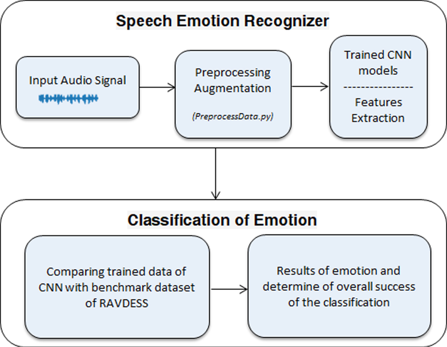
Flowchart of the system (own creation).
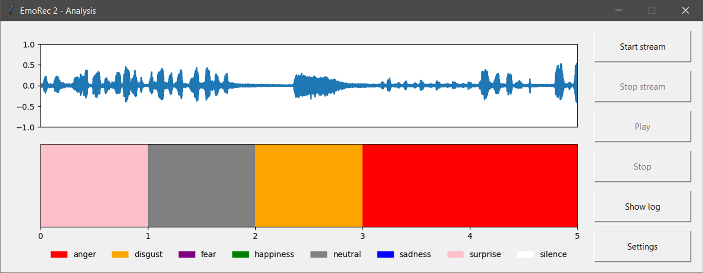
We have programmed our application with a graphical interface (see Fig. 2) in Python 3.6, whose task is to evaluate the data stream from the input device in real-time, for example, an audio stream recorded by a microphone. To create a graphical interface, we used the tkinter package in version 8.6, which is part of the standard Python library. The source code for this program is available on GitHub (given access is requested). For proper operation, it is necessary to first install these libraries (in parentheses is the version that we used during the creation of the program): matplotlib (3.1.1), sounddevice (0.3.13), soundfile (0.10.2), numpy (1.17.3), librosa (0.7.0), tensorflow-gpu (1.14.0) or tensorflow (1.14.0), keras (2.2.5), scipy (1.3.1).

Application window (own creation).
With the tensorflow-gpu library, it is also necessary to use Nvidia CUDA technology (we used CUDA version 10.0). The use of the tensorflow-gpu library is highly recommended because it reducex the CPU load during prediction.
The first step in processing the characteristics in EmoRec2 (see Fig. 2) is real-time analysis.
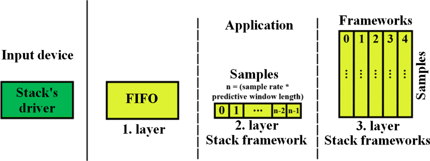
After selecting the input device (microphone) and setting other parameters (SettingsGUI), clicking the Start stream button (ControlPanelGUI) will start the analysis. The data stream from the selected device (StreamWorker) opens on a new thread (IOController). Incoming samples are stored in a stack before processing. Concerning speed, we have selected a three-layer stack (DataBuffer) for this purpose. The first layer consists of a FIFO structure, which is used to continuously transfer samples from the stack’s driver into our application. This structure is very fast, but it does not allow any other useful operations other than inserting and selecting samples. We used an implementation from the queue library. Samples are continuously taken from the first layer and moved over to the second layer, which is the frame stack - a standard indexed array. Its size depends on the settings of input parameters and is given as (sample rate * predictive window length). After obtaining the complete frame, the samples are moved to the third layer, which is a two-dimensional field. The last 5 frames are stored in this layer of the stack (older frames are discarded), the frame being considered the smallest, further indivisible, atomic unit (see Fig. 3).
Stack structure (own creation).
After inserting a new frame into the third layer, the processing of this frame on the new thread starts at the same time. Processing (PredictionController) must be performed in the same way as the pre-processing of the data on which the model was trained in experiment 2 - the frame is trimmed - silence is cut out at the end and the beginning, the frame is normalized to 60 dB volume, 13 MFCC characteristics, energy and zero-crossing are calculated using the Librosa library, the interpolation of the characteristics is performed, and finally the matrix with the characteristics is transposed. The model then predicts the emotion from this matrix, and the prediction is stored in a log (Logger) along with the start and end timestamps of the frame, using the time from the start of the analysis as the base time. Frame processing and prediction will not be performed if no sample in the frame exceeds -20 dB (reference value used by default by the amplitude_to_db() function in the Librosa library). In this case, the frame is saved in the log as silence. Finally, the graph is redrawn in the graphical interface (ControlPanelGUI). The first part of the graph plots 5 frames from the third layer of the stack, and the second part displays the 5 emotions from the log that were assigned to these frames (see Fig. 3). If the user of the application is interested in analyzing a file, instead of real-time audio input, after selecting the.wav file (wav format is required as it preserves all frequencies) from the disk (SettingsGUI), a Player will be created for him. The player automatically detects the sampling frequency of the file and loads all samples into memory. The sample is divided into frames (the value set in the Predictive window length field is used as the frame length). Preprocessing and prediction are performed sequentially for all frames in the same way as for real-time analysis (PredictionController). Again, the prediction results are written to the log (Logger). All frames together with predictions (ControlPanelGUI) are then drawn on the graph at once. The player also has the option to play the loaded file or stop playback (see Fig. 4).
EmoRec2 player with real-time emotion classification (own creation).
In the preprocessing, we prepared files for the extraction of various voice characteristics by normalizing and trimming the silence, and at the same time, we tried to correct some of the identified shortcomings. Part of the preprocessing was performed manually, and a part was automated using the PreprocessData.py script we wrote. Currently, the main hurdle with real-time classification is the small amount of input data and non-uniform classes. Getting new recordings (or creating your database) is time-consuming, so we had to find another way to expand the number of files. We decided not to combine databases - this would lead to even greater disruption of class uniformity. Instead, we’ve tried to solve these problems by modifying audio files, changing some of their properties while preserving their emotional content. This is how we got the new files that we added to the original ones. The databases also contain files that were useless to us - recordings of the emotion “peace” in the RAVDESS database and the emotion “boredom” in EMO-DB. We have omitted these files from further processing.
We also decided to only use the RAVDESS database to train our neural network. We have divided the files of this database into a training and testing subset in a ratio of approximately 8 : 2. Class uniformity and a large amount of data are especially important for the training of the classifier, so it was enough that we solved these problems only for the training subset of the RAVDESS database. The procedure we have proposed for this purpose relies on the existence of files from which new ones can be derived. For this reason, it is not possible to balance the uniformity of classes in the EMO-DB and SAVEE databases - the EMO-DB database lacks a whole class (surprise), and the SAVEE database does not contain any recordings of women. These databases did not interfere with the training process, and in addition to the test subset of the RAVDESS database, we used them to increase the robustness of testing - since the recordings have nothing to do with the training data used, they helped us get a better idea of classifiers’ success in real conditions.
After dividing the RAVDESS database, we had 76 files left in the training subset for neutral emotions and 152 files for all other emotions. At the beginning of the preprocessing, our goal was to obtain another 76 sets of neutral emotions so that their number was the same as the number of sets of other emotions.
In Adobe Audition, we used Stretch and Pitch features to lower the formant frequencies by two halftones. We used Batch Process and applied this function to all files of neutral emotion. New files were created, which differed from the old ones by a slightly different voice color and pitch. There was also a slight change in the pace of speech - the speech accelerated slightly and so the new files are a bit shorter than the original (by a few hundred milliseconds). This result was satisfactory for us because the files were changed enough to distinguish them from the original ones, but at the same time, they were not changed too radically.
We continued by trimming the silence from the files and normalizing their volume to a uniform level. This part of the preprocessing has been automated, and is part of the PreprocessData.py script, and is important for all three databases. We used functions from the Librosa library.
Many of the files in the used databases also contain stretches of silence. Since only short files were available and a common phenomenon is that the file contains, for example, 2 seconds of speech and 2 seconds of silence, these silent passages can significantly affect the voice characteristics that will be measured over the entire length of the file. However, we also had to take into account the possibility, that longer pauses between words can also be a factor that helps distinguish emotion, and cannot be simply cut out of the file. Therefore, we only trimmed silence at the beginning and end of the file, i.e. before and after the beginning of the speech. We used the trim() function from the Librosa library, which requires an input parameter specifying how many decibels the volume must be lower than the reference value to be truncated. The trim() function uses the maximum volume of the currently processed file as the reference level. We experimentally determined the value of the parameter at 28 dB.
The next step was to normalize the volume. The sound files were recorded under different conditions and using different microphones. Some features, such as input signal level can be significantly affected by the used microphone. The distance of the actor from the microphone also plays a role - the volume of the recording decreases with increased distance. This could lead to potential problems with attenuation of some energetic emotions (e.g. anger or joy) if the speaker is far away from the microphone or, conversely, to a large increase in intensity in emotions that are rather silent (e.g. sadness), if speaking too close to the microphone. We have tried to create a solution that will not depend on the use of specific hardware and a fixed distance from the microphone.
We decided to normalize the files using the normalize() function so that the average intensity of each file was 60 dB (at the reference value of sound pressure of 0.00002 Pa). The disadvantage of this approach is that we lose the dynamic volume range that could potentially help differentiate between different classes of emotions, but we gain the assurance that the input signal level will be the same regardless of the type of microphone or speaker distance.
It is a known fact that neural networks do learn the best when they have a large number of training samples available. Otherwise, they tend to slip into too much memorization of training data and poor generalization. This problem is called overtraining, or overfitting. One way to reduce overfitting is to get more data. Since we weren’t able to get brand new recordings, we tried to edit the files we had available. File modifications should be chosen to not only extend the original dataset but to reflect the various situations that a trained classifier may encounter later. This can be, for example, background noise or reduced quality. Conversely, an inappropriate modification would be to reverse the track, i.e. to play the file from the end to the beginning - it is very unlikely that the classifier will have to classify a person speaking in reverse. The process of editing files is called augmentation (see Fig. 5). Compensating for class uniformity is also a special case of augmentation. Here again, we only worked with the training subset of the RAVDESS database, and we were able to expand it to ten times its original size - we now have 10640 files. The first three augmentations from the following list were created manually in Adobe Audition, the others are the result of the PreprocessData.py script.

A comparison of spectrograms of various augmentations of a single file (own creation).
Explanation of Fig. 5: Original file, Decreased quality, distortion, echo, changed pitch, drop-out, white noise, background conversation, street noise, randomly added silence.
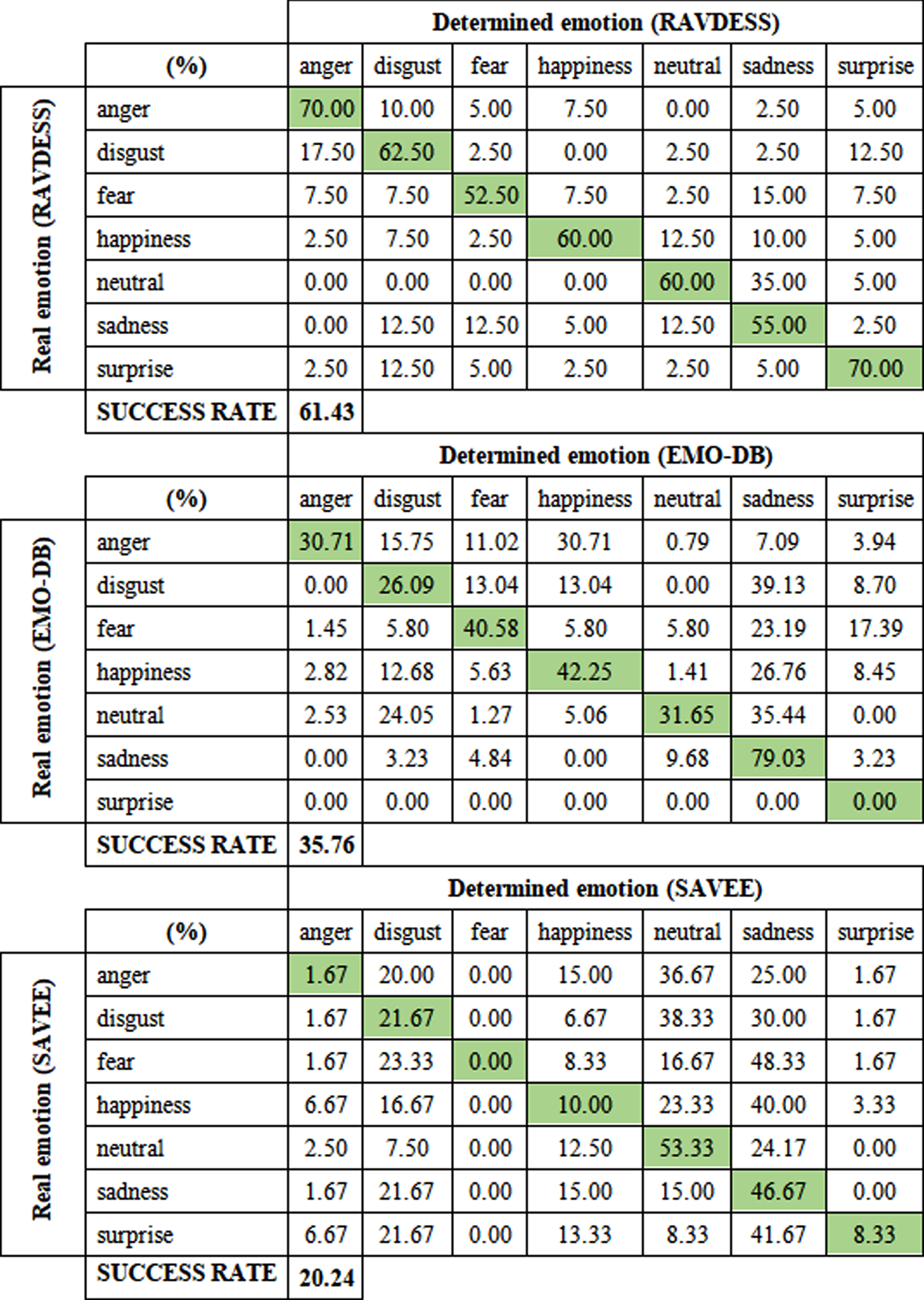
In preprocessing, we have prepared the files for the extraction of various voice characteristics, which will be used as input for neural networks. Our goal in this part of the experiment was to find the most suitable characteristics and the most suitable model architecture. Since EmoRec2 processes the characteristics in real-time, we had to pay attention to the simplicity of the extraction of the characteristics, the complexity of their further processing and the speed of prediction on unknown data in the experiments, in addition to the success rate of the model. We have used the keras library with a tensorflow backend to create and train the model. We have also used Nvidia CUDA technology to move the computing load of the training and prediction over to the Nvidia GeForce GTX 1050 graphics card. We have tested the created models using a test subset of the RAVDESS database, and EMO-DB and SAVEE databases. In each experiment, we processed the prediction results into the form of tables (see Tables 1–3), where we expressed the success of the classification as a percentage. The diagonal of the tables show the percentage of test cases that were determined correctly. The rows of the tables represent the emotions we have expected and the columns represent the emotions the model determined. To supplement, we have also created tables where we expressed success by the absolute number of correctly and incorrectly determined emotions.
Results of experiment 1 (own creation)
Results of experiment 2 (own creation)
Results of experiment 3 (own creation)

In the previous version of the application (EmoRec), we measured various characteristics using the PRAAT program - the fundamental frequency, the first 3 formant frequencies, the intensity, the jitter and the shimmer. From these characteristics, we then calculated the global characteristics. Now we have extended these characteristics to 5 formant frequencies, and we have added another characteristic - harmonics. We have used the parselmouth library for the measurement. Correct determination of formant frequencies proved to be problematic because it is first necessary to determine the maximum frequency –the upper limit of the frequency range in which the formant frequencies will be searched. The issue is that a suitable value of the maximum frequency is usually 5000 Hz for men, 5500 Hz for women and 8000 Hz for children. If we were to focus only on adults, then to achieve the greatest possible accuracy, it would first be necessary to correctly determine the sex. During training, we could very easily classify the files into men and women, but with real-time classification, it is not possible to determine the gender in advance. A potential solution could be to train another model that first determines gender, and the next step would be adapted to this prediction. Therefore, a simple solution was to set the maximum frequency to 5500 Hz, which provides a sufficient frequency range for both women and men, but the formants in the case of men may differ slightly from their actual value.
After extracting the characteristics, we determined the maxima, minima, standard deviations, medians and other values –a total of up to 64 global characteristics for each set. We scaled each variable to values in the interval between 0 and 1. For this scaling, we have used the MinMaxScaler() function from the scikit-learn library. We tried to reduce the number of variables by identifying unnecessary variables. We excluded characteristics with a degree of mutual correlation above 90%. The high degree of correlation between the two characteristics indicates that these characteristics carry the same information, so using one of them is enough. We determined the degree of correlation with the corr() function from the pandas library, which uses Pearson’s correlation coefficient as the default method. At the end of the preparation, we still had 45 variables left. The preparation was automated by our Ex1_prep.py script.
The feedforward neural network model, network architecture, and activation functions are shown in the following figure (see Fig. 6). We have tried to reduce the overfitting by the dropout technique - some neurons accidentally fall out, and the network is forced to better generalize. We have programmed the Ex1_NN.py script to create and train the model.
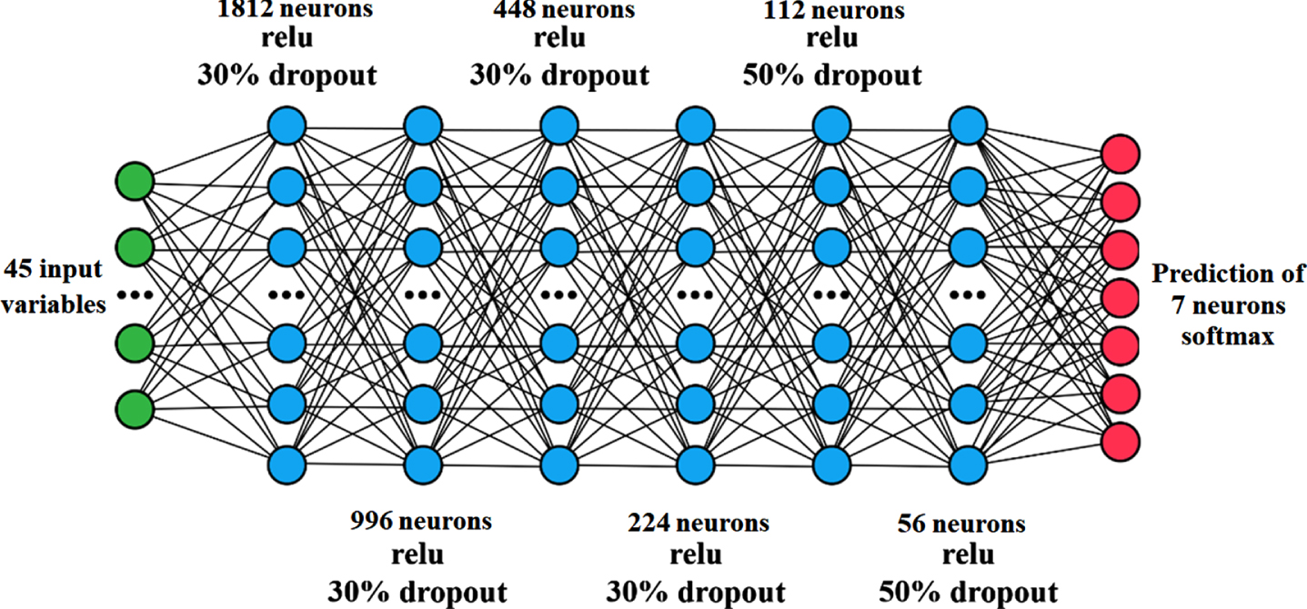
Feedforward neural network architecture (own creation).
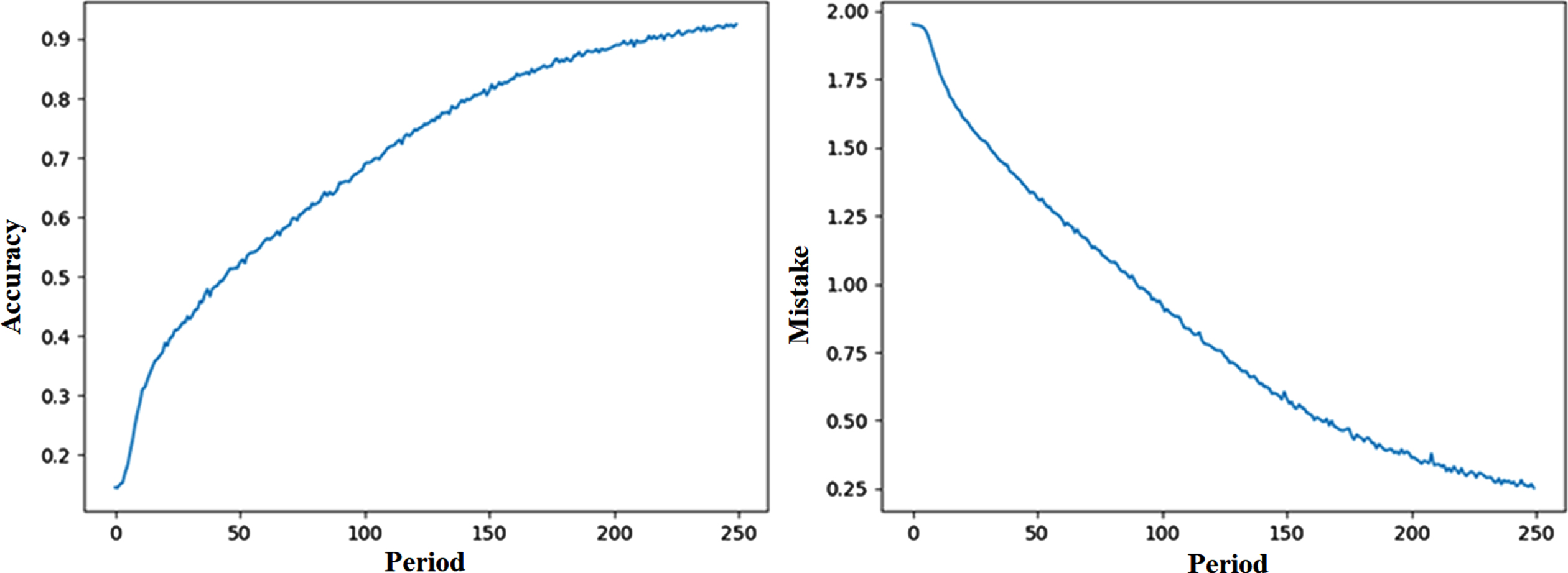
The training of the network ran for 250 epochs. We used Adam optimizer with a learning speed of 0.00005. We have used categorical cross-entropy as an error function. The figure below (see Fig. 7) shows the course of training and error reduction.
Experiment 1 –the course of training and error reduction (own creation).
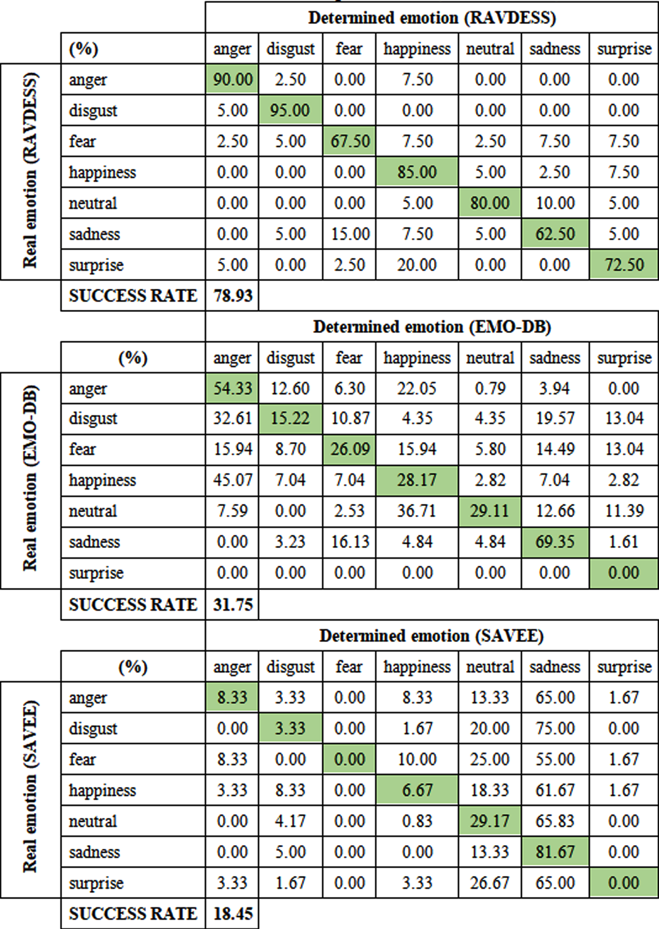
The model in the test with the RAVDESS database achieved an overall success rate of 61.43% (see Table 1). All emotions were correctly determined in more than 50% of cases, with the most accurate being the emotions of anger and surprise - up to 70%.
The least accurate was the prediction of fear - 52.50%, while fear was incorrectly defined as sadness in 15% of cases. We observed the highest degree of confusion for another individual category in neutral emotions, which is up to 35% of cases were incorrectly classified as sadness.
The test using the German recording database (EMO-DB) turned out to be less satisfactory than the previous test (see Table 1). The model predicted the actual emotion in 35.76% of recordings. The most successful classifications were achieved in the case of the emotion of sadness –79.03%, but other emotions were increasingly confused with this emotion. We observed the lowest accuracy in disgust –26.09%. Surprise recordings are not in this database, so the last row of the table is filled with zero values.
The test with the SAVEE database turned out the worst, the overall success rate was only 20.24% (see Table 1). Most predictions were divided into 3 categories - neutral emotion, sadness and disgust. The remaining 4 emotions were perceived only minimally by the model, while fear was not correctly determined even once, and at the same time, no other emotion was incorrectly classified as this emotion.
Experiment 2 –1D convolutional network
In this experiment, we measured 13 MFCC characteristics and added the energy value and zero-crossing to them. This time we did not calculate global characteristics from the characteristics, but we used their local values measured over time. We used the mfcc(), rms() and zero_crossing_rate() functions in the Librosa library for extraction. We have set the input parameters of these functions. We set the length of the fast Fourier transform window to 800 samples, and the number of samples between successive frames to 400. We automated the extraction of characteristics and their subsequent processing in our Ex2_prep.py script.
The main issue with this method is that the 15 selected characteristics are measured over time. The result of the measurement is a matrix of 15xN, where N depends on the length of the input file (with the input parameters used, it is approximately 100 samples per 1 second). Although keras library supports the variable size of the input to the convolutional neural network, the first prediction after resizing may take up to a few seconds - this would not be appropriate for real-time determinations. The graph of the function formed by the local values of the character over time can be as needed to be resampled to a fixed length so that its shape is preserved. This goal is achieved by selecting the number of points on the continuous function graph that corresponds to the desired length, and then creating a new graph by interpolation that coincides with the original graph at the selected points. To do this, we used the interp1d() class, which is part of the scipy library. We decided to use cubic interpolation because experiments have shown that it retains the shape of the original graph more faithfully than linear interpolation. We have scaled the characteristic graphs to 256 samples. Finally, we scaled each characteristic to values in the interval between 0 and 1 (see Fig. 8). Again, we used min-max scaling. From the entire training subset of the RAVDESS database, we found the absolute maxima and minima for each of the 15 characteristics. Then we scaled the training and test subset based on them, as well as the other two databases. At the same time, we saved these maxima and minima to a file, because in the final program, the scaling must take place in the same way and based on the same values as on the data with which the model was trained.

An example of resampling and scaling - the shape of the function is unchanged (own creation).
Explanation of Fig. 8: Graph of energy before adjustment, Graph of energy after resampling to 256 samples, Graph of energy after min-max scaling.
The very last step was to transpose the matrix of characteristics from 15x256 to 256x15. Transposition was necessary for a simple reason –a neural network created using the keras library for proper operation requires a matrix, where columns represent characteristics, and rows of the value of these characteristics over time, while the librosa library provides output in the opposite form.
The local values of 15 characteristics are the input of the neural network. For this type of input one-dimensional convolutional networks are suitable to be used. The network architecture is shown below (see Fig. 9). We used 4 convolution layers, each followed by a pooling layer and normalization. At the end of the network, we have added one fully connected layer. We reduced learning by l1 and l2 regularization (weight penalty), and dropouts.
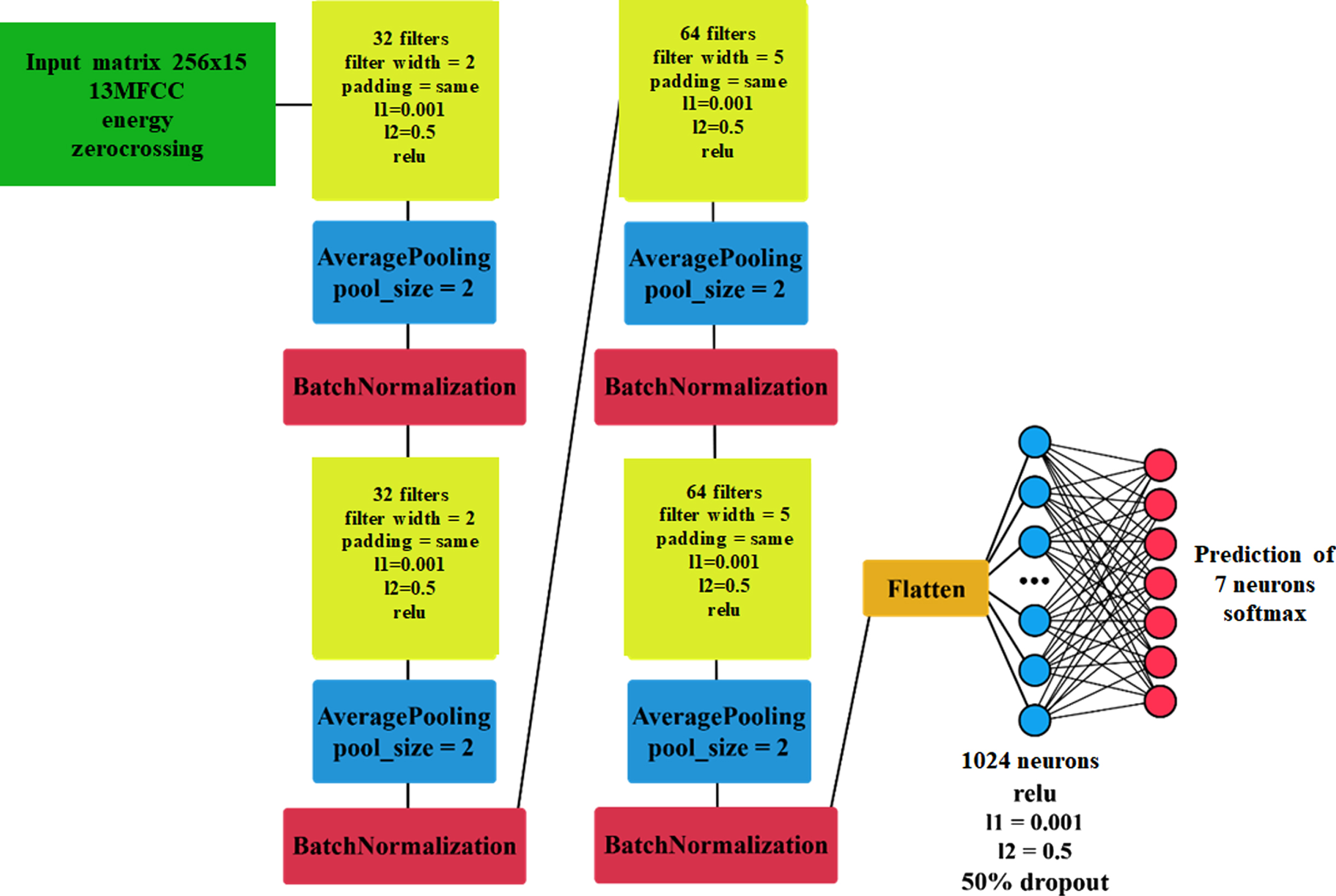
1D convolutional network architecture (own creation).
We have trained the network using Adam optimizer with a learning speed of 0.00005 for 150 epochs. As the error function, we have once again used categorical cross-entropy. The accuracy and error rates during each epoch are shown in the following figure below (see Fig. 10).

Experiment 2 –the course of training and error reduction (own creation).
Using the RAVDESS database and this model, we have achieved a success rate of 78.93% (see Table 2).
The success rate of determining any category did not fall below 60%, 4 out of 7 categories were correctly determined in more than 80% of cases. The most significant mistake was in the emotion of surprise, which for 20% of cases was determined as happiness. The model tested with the EMO-DB database (see Table 2) did not achieve the success rate of the previous test. Only two emotions were correctly determined to be higher than 50% - anger and sadness. The model achieved an overall success rate of 31.75%. The test with the SAVEE database turned out to be the worst once again (see Table 2). Most recordings were determined as sadness or neutral emotion. The prediction of the other classes was negligible. Even emotions that are usually strong and energetic (such as anger) have in most cases been identified as sadness.
Experiment 3 –2D convolutional network
In the last experiment, we used a graphical representation of sound files - spectrograms - as input for a neural network (see Fig. 11).
We calculated the spectrograms with the melspectrogram() function in the Librosa library. These spectrograms show the frequency-converted from Hz to mel units on the y-axis. We have set the frequency range for the calculation of spectrograms to an interval of 50 to 4000 Hz. The parameters of the fast Fourier transform were the same as in experiment 2. We then saved them in.png image format. In the case of spectrograms, the same problem occurred as in the previous experiment. The dimensions of the spectrogram depend on the length of the audio file. Therefore, we adjusted their dimensions to 128x128 pixels. We wrote the script Ex3_prep.py to create spectrograms. Thus, the input for the neural network was a matrix of spectrograms with dimensions 128x128x3. The third dimension of the matrix is color channels (RGB) dimension. This method has proven to be memory intensive and it was not possible to load all of the training files at once. We used the ImageDataGenerator class from the keras library, and we have loaded the images in increments of 32. We then normalized the pixel values between 0 and 1 by setting the generator’s rescale parameter to 1/255. We used l1 and l2 regularization to reduce overfitting. Each convolution layer was followed by a pooling layer and normalization. We created the model (see Fig. 11) using the Ex3_NN.py script.

2D convolutional network architecture (own creation).
The model was trained for 10 epochs using the Adam optimizer and learning speed of 0.00001. We have used the categorical cross as the error function. The figure (see Fig. 12) shows the accuracy and error during the epochs.

Experiment 3 –the course of training and error reduction (own creation).
In the test with the RAVDESS database, we have achieved an overall classification success of 75.71%. Each of the 7 emotional states was correctly identified in more than 60% of cases. However, the overall success rate for any of the emotions did not exceed 90% (see Table 3).
In the test with the EMO-DB database, the model correctly determined the emotion in 25.49% of recordings. This test was characterized by a high degree of misidentified emotions. We observed an increased success rate only with fear and neutral emotions (see Table 3).
In the test with the SAVEE database, the model once again correctly classified only the minimal amount of emotions, a total of 22.02% of cases. Most were determined as sadness, disgust, or surprise. The emotional state of anger and fear was not recognized after training the neural network at all (see Table 3).
Discussion –evaluation of experiments
The behavior of the models in the tests showed that they were best able to recognize the emotions in the recordings that came from the same database using which they were trained (RAVDESS). In the tests with the remaining two databases, the prediction success was much lower. The success of the model is strongly dependent on the quality of the input data. The model is not applicable in practice if it has been trained on recordings that are not a sufficient reflection of the manifestations of emotions in reality. The recordings came from the RAVDESS, EMO-DB and SAVEE databases for model training, which despite their popularity in the scientific community, lack diversity. They are limited to two very similar English sentences, are about the same length, and were recorded by a small group of actors who do not represent all ages. Besides, there is only a small sample of recordings - the training subset consists of 1,064 files, which amounts to 152 files per emotion. We were able to increase their number by augmentation, but the files obtained in this way are only a slight modification of the original ones, and therefore do not present a solution for other shortcomings. A better solution would be to obtain a database of completely new recordings, in which there would be more files than in the RAVDESS database, and at the same time would contain all the emotions of Ekman’s classification for both sexes. One option is to try to obtain recordings from call centres or other similar sources. The advantage would be that they would capture people’s behavior and emotions in real situations. The issue would be the protection of privacy or copyright, as well as the low quality of recordings. Such recordings would probably need to be categorized (i.e. having emotions assigned to each recording) with the help of a psychologist. Another way to get more recordings would be to create our database, for example with the help of theatre actors. This would require the collaboration of experts from several fields - psychology, linguistics and sound engineering. For this newly created database to be beneficial, it would have to contain a much larger number of recordings (tens to hundreds of thousands) than are found in existing databases. Furthermore, such a database would have to contain recordings of sentences of various lengths and should be recorded in very good quality - if necessary, it is easier to decrease quality files than to try to salvage low-quality ones. It is also necessary to pay attention to the uniformity of classes. Creating such a large database in one language can be problematic, so a database of several related languages should be created - for example, a Slovak-Czech-Polish database. The process of creating a new database is likely to be time and financially consuming, but the availability of such a database would be a major step forward in machine emotion recognition, as the model would be forced to find much more universal rules in training to avoid overfitting and would be much more suited for real situations.
In choosing the best model and methodology, we also had to take into account the time it takes to extract and process the characteristics from the input, and how long the subsequent prediction of emotion takes. For each input recording, we have tried to measure approximate processing and prediction times using the Python time library. From the obtained times, we then calculated the average processing and prediction times for one recording. The results are in the table below (see Table 4).
The average speed of processing and prediction (own creation)
The average speed of processing and prediction (own creation)
The method from experiment 2 proved to be the most suitable because it is the fastest, input processing was simple and seamless and it has achieved the highest overall success rate. The slow processing by the parselmouth library speaks against experiment 1, as well as its lowest success rate and the accuracy of the determination of formant frequencies influenced by gender. Experiment 3 did not surpass the success of experiment 2. Moreover, the processing was several times more time-consuming. Therefore, we have decided to use the model created in experiment 2 for our EmoRec2 application.
Our best-achieved result of the overall classification success rate was 78.93% when applying RAVDESS to a 1D convolutional neural network supports the results presented by Stolar et al [21], achieved using his experimental solution in the Matlab environment. Stolar has achieved a different success rate of 79.68% for women and 76.79% for men by combining a convolutional network and an SVM classifier separately for each. However, the combination of the convolutional network and SVM was less accurate in classification (73.84% for women and 72.73% for men) than our model. Our model approaches the results of Cen et al [22] research, where their SVM classifier classified 4 emotions (anger, happiness. Sadness. Neutral emotion) with a total success rate of 78.78% in real-time.
We have tried 3 methods of classifying emotions. Their common feature is that the prediction success was always highest in tests with a test subset of the RAVDESS database, while the best overall result was achieved in the second experiment –78.93%. Tests with the EMO-DB database were successful at 35.76%. 31.75% and 25.49%. In all three experiments, the worst results were obtained in tests with the SAVEE database. We conclude from these results that characteristics which we researched contain sufficient information about the emotional context of the recording. However, the models we proposed could not derive sufficiently general rules, which would be valid for all databases. The cause of this is, that we have used only a subset of the RAVDESS database for training. In this database, the recordings consist of only 2 repeated sentences, which also are very similar. For further research, this reveals the need to obtain a larger number of diverse recordings. More diverse recordings can be obtained by creating a new robust database of sound samples. This database, however, doesn’t currently exist.