Color multi-focus image fusion based on transfer learning

Abstract

Multi-focus image fusion is a technique that integrates the focused areas in a pair or set of source images with the same scene into a fully focused image. Inspired by transfer learning, this paper proposes a novel color multi-focus image fusion method based on deep learning. First, color multi-focus source images are fed into VGG-19 network, and the parameters of convolutional layer of the VGG-19 network are then migrated to a neural network containing multilayer convolutional layers and multilayer skip-connection structures for feature extraction. Second, the initial decision maps are generated using the reconstructed feature maps of a deconvolution module. Third, the initial decision maps are refined and processed to obtain the second decision maps, and then the source images are fused to obtain the initial fused images based on the second decision maps. Finally, the final fused image is produced by comparing the Q^ABF metrics of the initial fused images. The experimental results show that the proposed method can effectively improve the segmentation performance of the focused and unfocused areas in the source images, and the generated fused images are superior in both subjective and objective metrics compared with most contrast methods.

Keywords

Deep learning feature extraction multi-focus images fusion neural networks transfer learning

1 Introduction

Due to the limitations of natural and physical conditions, it is difficult for the ordinary optical digital camera to capture images with all-in-focus, simultaneously. Multi-focus image fusion can integrate the focused areas of different source images into a fully focused image, resulting in more complete information and better visual effects [1 –6]. As an important branch of image fusion, multi-focus image fusion has been widely used in computer vision [7], macrophotography [8], microscopic imaging [9], mobile applications [47], and other applications [48 –50].

In the past decades, many multi-focus image fusion methods have been proposed, which can be broadly divided into two categories: conventional methods and deep learning-based methods. There are some well-known conventional methods, such as wavelet transform [10], crossover bilateral filter (CBF) [11], discrete wavelet transform (DWT) [12], discrete cosine harmonic wavelet transform (DCHWT) [13], dual-tree complex wavelet transform (DTCWT) [14], curvelet transform (CT) [15], and non-subsampled shearlet transform (NSST) [16]. In these methods, the source image is first decomposed to obtain a set of sub-images representing the information of space and frequency. Then, the sub-images of different source images are fused by a certain fusion rule. Finally, the inversion transformation is performed to obtain the fused image [51]. However, most of these methods are relatively complex and have certain limitations in terms of feature extraction and fusion strategy. Besides, most conventional methods are limited in the performances and may produce unexpected artifacts.

With the rise of computing device and theory, deep learning is showing strong power in both industrial and academic fields. Therefore, many multi-focus image fusion methods based on deep learning have emerged. Du et al. [17] proposed a multi-focus image fusion method based on image segmentation and multi-scale convolution neural network. This network performs multi-scale analysis on each input image to obtain independent feature maps on the boundary of focused and unfocused regions. Then, these feature maps are fused to generate the fused feature map. After initial segmentation, morphology, watershed and other post-processing operations, the final fusion decision map is then obtained. Tang et al. [18] proposed a multi-focus image fusion method based on a neural network, they firstly set the corresponding fusion labels on the samples of dataset according to different focus levels, and then the p-CNN was trained to measure the focus level of each pixel for fusing them. Li et al. [22] proposed a method to respectively fuse the chromaticity and luminance components of the color multi-focus images in YCbCr space. In Li’s method, a U-net was trained to fuse the luminance components in YCbCr space by a hybrid objective function containing L1 loss and SSIM loss. Besides, a weighting strategy was used to merge the chromaticity components in YCbCr and obtain fused images. Li and Guo et al. [19] proposed deep regression pair learning (DRPL), which divided the input image into some small patches and applied a classifier to judge whether the patch was the focused or unfocued areas, and used the DRPL directly to convert the whole image into a binary mask. Liu et al. [18] utilized Haar wavelet and simple fusion rules to propose a fusion algorithm that was suitable for hardware implementation. Jung et al. [19] proposed an unsupervised deep image fusion network (DIF-Net), which parameterized the entire processes of image fusion to generate an output image that had an identical contrast to high-dimensional input images.

However, deep learning based methods always require a large datasets of labeled images to train the model, but there are not so many natural image datasets for model training in multi-focus image fusion. Thus, the collection and production of large datasets becomes a time-consuming and laborious task; besides, the large datasets have high requirements on machine hardware to train models and have high time costs in model training. Thus, the applications of conventional deep learning-based methods are limited in many field of image fusion.

Fortunately, transfer learning can be used to address these problems in conventional deep learning based methods. In transfer learning, the source task usually has a large number of training samples, and the target task usually has limited training samples. Therefore, the knowledge and feature extraction ability learned from the source task can be employed to improve the performance of the target task. In this way, we do not need to retrain a new model with a large amount of training data to complete the target task. In image fusion, it is difficult to produce a large number of training samples to train a deep learning model. Therefore, a novel color multi-focus image fusion method is proposed based on transfer learning, which also exploits the advantages of deep learning to achieve competitive performance based on a pre-trained model (VGG-19). The contributions of this paper are presented as follows:

This paper proposes a novel transfer learning-based color multi-focus image fusion method by combining deep learning model, in which the VGG-19 network is transferred into our newly defined model for feature extraction.

An efficient network structure is designed for feature reconstruction that is used to generate the fusion decision maps; besides, a layer-by-layer hybrid loss function is introduced to better supervise the training and improve the robustness of the network.

Unlike most previous methods based on image patches or blocks [18], this work makes pixel-level predictions for both focused and unfocused areas in an entire source image to fuse them.

The remainder of the paper is divided into four sections. The second section briefly describes transfer learning and the VGG-19 network. The third section details the proposed method. The fourth section analyzes the experimental results. The last section summarizes this paper.

2 Related work

In this section, we briefly introduce the background knowledge about convolutional neural network and transfer learning. In addition, since our transfer learning network is based on VGG-19, we first briefly describe the VGG-19 network model.

2.1 Convolutional neural network

Convolutional neural network (CNN) is one of the most representative models in deep learning, and it has made many breakthroughs in image processing. The convolutional layer is the crucial component of CNN, which extracts the specific features of the image by the different sizes of the convolution kernels. After applying the convolutional layers several times, a set of feature maps of input images can be extracted. Let C_i represent the feature map of the i-th layer in our network, then the C_i can be generated as follows: $C_{i} = M (C_{i - 1} * W_{i}),$ (1) where C_i denotes the feature map of the current network layer, C_i - 1is the feature map of the previous layer, W_i is the weight of the i-th layer, symbol “*” denotes the convolution operation and M (.) is the Mish activation function [43], and expression of Mish activation function as follows: $Mish (x) = x * Tanh (ln (1 + e^{x})),$ (2) where T (.) is the Tanh activation function and its expression as follows: $Tanh (x) = \frac{e^{x} - e^{- x}}{e^{x} + e^{- x}},$ (3)

2.2 Transfer learning

Because of the excellent performance, the transfer learning (TL) [23, 33] is now widely used in computer vision [36], text classification [34], natural language processing [37], medical image processing [35], and other fields.

Given a source domain D_S and source task T_S a target domain D_T and target task T_T, TL aims to improve the learning performance of the target predictive function f (□) in D_T using the knowledge in D_S and T_S, where D_S ≠ D_T, or T_S ≠ T_T [23].

The main idea of TL is to apply knowledge or patterns learned from a domain or task to another related domains or problems. By transferring the labeled data or knowledge from source domain, and the learning efficiency and performance of the target domain or task will be improved. Generally, TL can be divided into four categories according to transferring way: instance-based TL, feature-based TL, parameter/model-based TL, and relation-based TL. Parameter/model-based TL is a transfer method to find the parameters shared between the source and target domains. This transfer way has an assumption that the data in the source domain and the target domain can share some important model parameters. This work is a parameter/model-based TL model that is transferred from the VGG-19 network.

Since the VGG-19 network has been trained to learn excellent feature extraction capabilities with stable network parameters, we transferred its convolutional layer parameters and rebuilt a new hybrid network based on the transferred parameters for fine-tuning, thus our network inherited the VGG-19 parameters and had excellent feature extraction capabilities. Figure 1 describes our idea of transfer learning in this work.

Fig. 1

Our idea of transfer learning.

2.3 VGG-19 network

The VGG [24] network is a very classic model in the field of deep learning, proposed by the Visual Geometry Group at Oxford University.

The VGG network was trained on a massive image samples and widely-used in many fields. The VGG network has two architectures as: VGG-16 and VGG-19, and this paper implements TL based on the VGG-19 to complete the multi-focus image fusion task. The VGG-19 contains 16 convolutional layers, five max-pool layers, two fully connected layers and a Softmax layer.

3 The proposed method

In this section, the proposed method is introduced in detail. Firstly, we introduce the overall processes and network architecture; meanwhile, the feature extraction and feature reconstruction module, as well as the implementation of TL are explained. Then, we provide the definition of the loss function.

3.1 Overall processes and framework

The proposed network consists of two parts: feature extraction module, and feature reconstruction module. The network architecture is shown in Fig. 2, and the steps are shown as follows:

Fig. 2

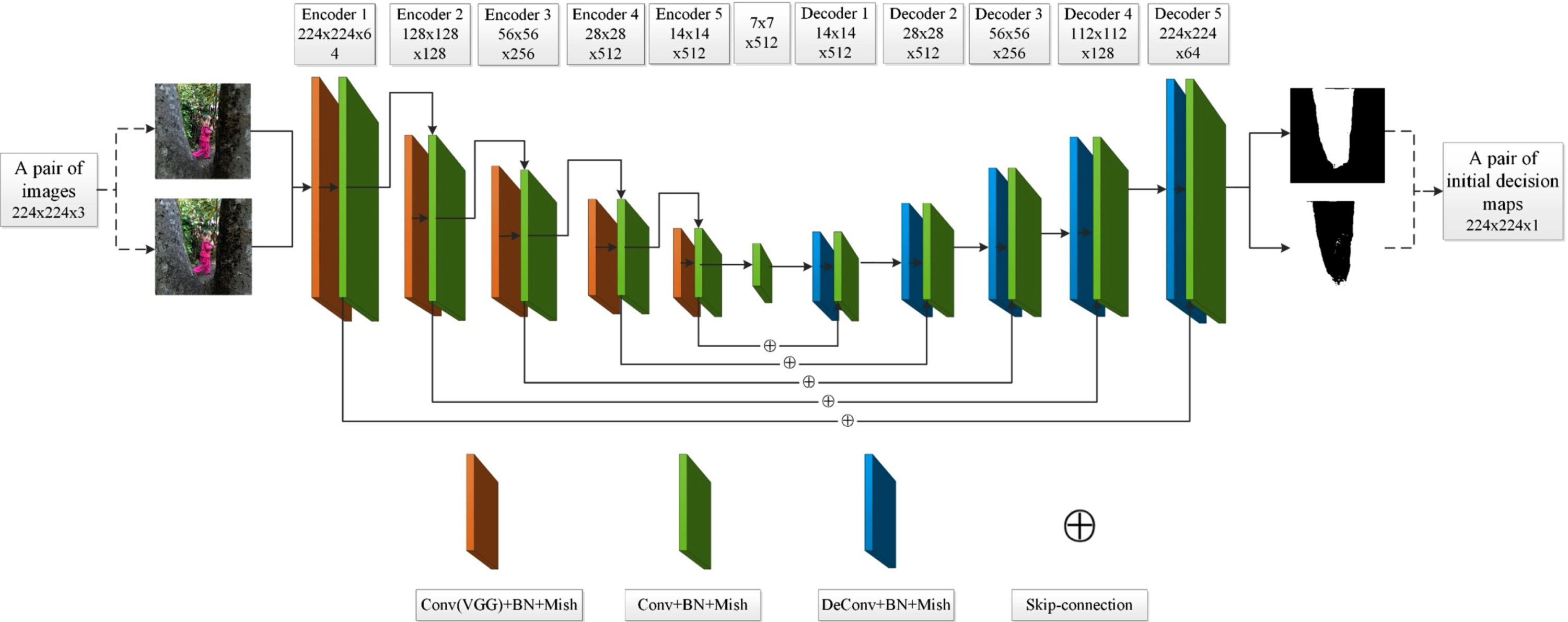
The proposed network architecture.

A pair of color source images (224×224 pixels) are fed into the pre-trained VGG-19 network for initial feature extraction.

The convolutional layer parameters of the VGG-19 network are transferred into our designed feature extraction module to get the feature maps.

The obtained feature maps are input into the feature reconstruction module that can generate the initial decision maps.

The initial decision maps are processed by logical operation to obtain second decision maps, and pixel-level fusion process is performed based on the second decision maps to obtain the corresponding initial fused images.

The Q^abf metric of the initial fused images are calculated respectively, and the fused image with the higher Q^abf metric are output as the final fused image.

3.2 Feature extraction module and transfer learning implementation

In Fig. 3, the feature extraction module has five Encoders, in which the Encoder 1 and Encoder 2 have the same network structure, and the Encoders 3, 4 and 5 have the same network structure. Both the Encoder 1 and Encoder 2 contain seven convolutional layers, in which the first two layers (the orange layers) are the transferred convolutional layers from the VGG-19 network, thus the word “VGG” is marked to indicate them. The next five layers are routine convolutional layers defined by us for depth feature extraction, in which do not have the word “VGG”. Encoders 3, 4, and 5 all contain nine convolutional layers, and their network architectures are the same as Encoders 1 and 2, in which the first four layers are convolutional layers transferred from the VGG-19 network and the last five layers (the green layers) are routine convolutional layers. Thus, the naming way of convolutional layers in Encoders 3, 4, and 5 are the same as Encoders 1 and 2.

Fig. 3

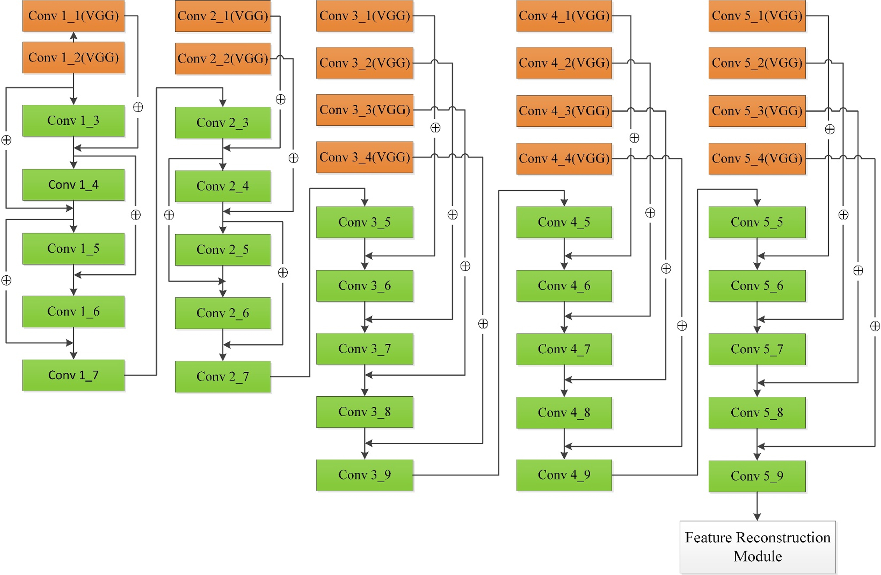
Feature extraction module.

Firstly, the source images are inputted into the pre-trained VGG-19 network for initial feature extraction. Secondly, all the parameters of the VGG-19 networks convolutional layers are correspondingly transferred into our designed network. Thirdly, the transferred convolutional layers and our newly designed layers are combined for secondary feature extraction. The VGG-19 network has been trained on a massive dataset and has achieved excellent results in many fields that can be regarded as source domain, thus we transfer the parameters of the pre-trained VGG-19 network into our model to apply them for color image fusion (target domain). In this method, the transferred VGG-19 network is used to segment the focused and unfocused areas in the source images, which can be regarded as a parameter/model based TL. The source images are inputted into the network, and five Encoders are used for feature extraction.

Thus, after the processing of each Encoder, the size of the feature maps will become quarter of the original images, and the size of the feature maps of the feature extraction module is reduce to 7×7 pixels from the initial 224×224 pixels. To retain more detailed information of the source images, we employ the convolution operations instead of the pooling operations to reduce the dimensionality of feature maps. In the last layer of each Encoder, we set the size of its convolution kernel as 3×3, the stride is set as 2, the padding is set as SAME. In addition, in the feature extraction module, except for the last convolutional layer of each Encoder, we set the size of the convolution kernels of all other convolutional layers as 3×3, strides is set as 1, padding is set as SAME.

Figure 4 shows the structure of Encoder 1, in which each convolutional block consists of a convolutional layer, a Batch Normalization (BN) layer, and a Mish activation function layer. Similarly, the convolutional blocks of the other Encoders have the same structure, in which each convolutional layer followed by a BN layer and a Mish activation function layer.

Fig. 4

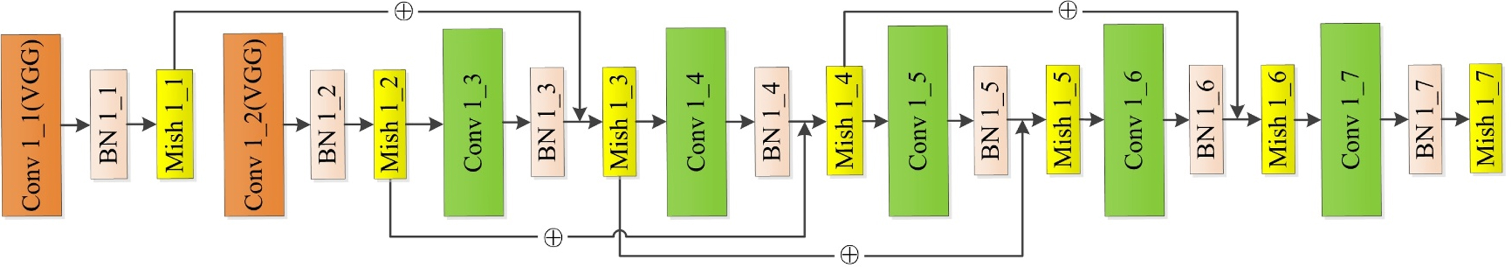
Encoder 1.

3.3 Feature reconstruction module and skip-connection

The adopted feature reconstruction module and skip-connection is introduced in this sub-section.

3.3.1 Feature reconstruction module

In Fig. 2, the feature reconstruction module also includes five Decoders that is corresponding to the feature extraction module. Decoder 1, 2 and 3 have the same network structure, which are composed of one deconvolution layer and eight feature reconstruction convolution layers. The Decoder 4 and Decoder 5 have the same network structure, they are composed of one deconvolution layer, and six feature convolutional reconstruction layers. In the Decoders, a BN layer and a Mish activation function layer follow each deconvolution layer and each convolutional layer.

In Fig. 5, the feature maps outputted by the feature extraction module will be inputted into the Decoders of the feature reconstruction module for feature reconstruction. After each deconvolution layer, the size of feature map will be expanded to quadruple of the original size, and the feature maps will be fused with the corresponding feature maps in the feature extraction module, and then the feature maps are fed into the next feature reconstruction convolutional layer combined by the skip-connection structure. The size of the final output feature maps was expanded to 224×224 from 7×7, and the size is the same as that of the original map and source images. The predicted map has only two values, as 0 and 1, which is regionally distributed and represent the focused and unfocused areas of the source image. At last, the loss function is used to analyze the errors between the predicted map and the label image (Ground-Truth). In the all Decoders, the size of all deconvolution kernel is set as 4×4, and the strides is set as 2, padding is set as SAME. The size of all convolutional kernel is set as 3×3, and the strides is set as 1, and padding is set as SAME.

Fig. 5

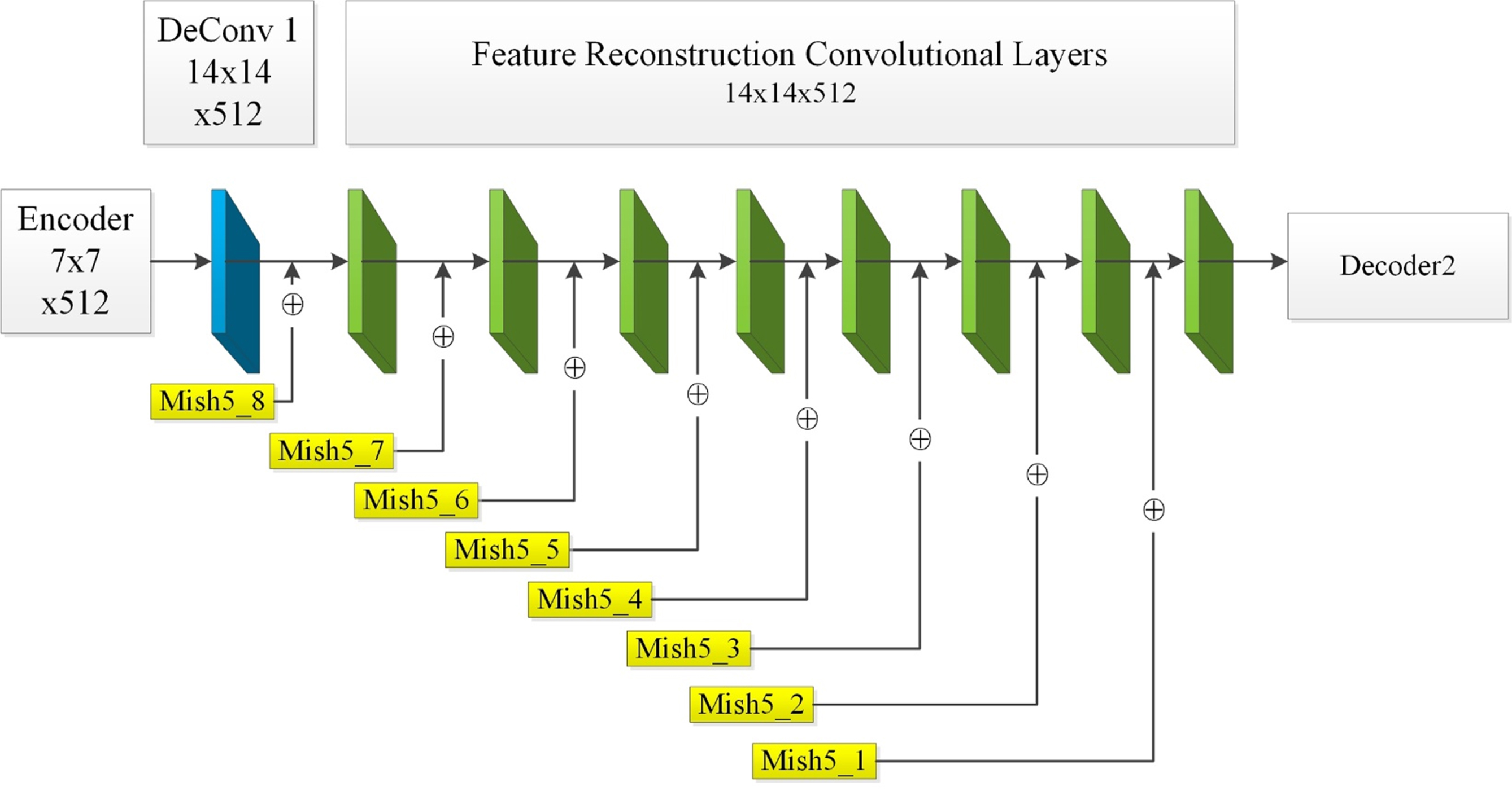
Decoder 1.

3.3.2 Skip-connection structure

As shown in Figs. 2, 3, the layers marked by arrow are concatenated to input the feature maps into the next layers. By the skip-connection operations, the low-level and high-level features are integrated, allowing the network to retain more detailed information. In addition, the skip-connection can effectively overcome the problem of gradient disappearance and network degradation while the network deepens.

The operation of skip-connection is shown as follows: $y_{i} = h (x_{j}) + M (C_{i - 1} * W_{i}),$ (4) where h (x_j) denotes the feature mapping of the j-th layer, C_i - 1 is the feature map output from the (i-1)-th network layer, W_i is the convolution kernel parameters of the i - th layer, M (□) is the Mish activation function, and y_i is the feature map input into the i - th layer.

3.4 Loss function

In this work, the label “1” is used to mark the unfocused areas in the source images; conversely, the label “0” is used to mark the focused areas. In model training, we assume the network has learned the distribution of the label images when the loss function stabilizes at a sufficiently small interval. To better supervise the learning of the network, we use the layer-by-layer hybrid loss function to train our network. That is to say, in the feature reconstruction module, we put the feature map output by each Decoder into the loss function and calculate the loss value with ground-truth, and the weighted average of the five loss values is our final loss value. Our network uses a hybrid loss function that combines cross entropy loss and L2 loss, and the hybrid loss function is formulated as: $L o ss Function = \frac{1}{n} \sum_{i = 1}^{n} (l_{1}^{i} + l_{2}^{i}),$ (5) where n is the number of decoders, and the value of n is 5 in this paper, $l_{1}^{i}$ is the i - th loss value of the cross entropy loss function, and is formulated as: $S_{i} = \frac{e^{V_{i}}}{\sum_{j} e^{V_{i}}},$ (6)

$l_{1} = L_{Cross Entropy} = - \frac{1}{k} \sum_{i = 1}^{k} y_{i}^{'} log (y_{i}) .$ (7)

$l_{2}^{i}$ is the i - th loss value of the L2 loss function, and its expression as follows: $l_{2} = L_{L 2} = - \frac{1}{k} \sum_{i = 1}^{k} {(f (x_{i}) - y_{i}^{'})}^{2},$ (8)

In Formula 6, the Softmax function is used to normalize the output components that is corresponding to each category of the network, its output is a probability that the input data belongs to each category.

In Equation 7, $y_{i}^{'}$ is the i - th value in the label, and y_i is the corresponding component in the vector normalized by the Softmax function, k is the number of batch-size. In Equation 8, f (x_i) is the predicted value of the i - th image of our network, and $y_{i}^{'}$ is the true value of the label of the i - th image.

4 Fusion strategy

Our TL-based model first outputs a pair of initial decision maps M₁ (i, j) and M₂ (i, j) that are corresponding to the source image S₁ and S₂. The initial decision maps are a pair of binary images that only have 0 and 1, where the black area is 0 and the white area is 1, marking the focused and unfocused areas of the source image S₁ and S₂, respectively. While the initial decision maps generated by our model can accurately predict most of the focused and unfocused areas in the source images, there may be some prediction errors, such as Fig. 6(a) and (b).

Fig. 6

Initial decision maps and secondary decision maps.

To solve this problem, we propose a sample method to integrate the decision maps and produce the fused images. We take a pair of source image as an example that is shown in Fig. 6, the initial decision maps are respectively M₁ (i, j) and M₂ (i, j), and the secondary decision maps are respectively M₄ (i, j) and M₅ (i, j). In this method, a logical operation is first used to refine the initial decision maps, resulting in a second pair of decision maps M₄ (i, j) and M₅ (i, j), such as Fig. 6(c) and (d). Secondly, the decision maps M₄ (i, j) and M₅ (i, j) are respectively used to produce the fused images F₁ (i, j) and F₂ (i, j). Thirdly, the Q^ABF metric of the fused images F₁ (i, j) and F₂ (i, j) are computed, respectively. Finally, we take the fused image with the higher Q^ABF metric as the final fused image, thus the decision map M₄ (i, j) in Fig. 6(c) is selected to produce the result.

The proposed operation is shown as the Pseudo-Code of Fusion Strategy. $\begin{matrix} Pseudo - Code of Fusion Strategy \\ - - - - - - - - - - - - - - - - - - - - - - - - - - - - - - - - - - - \\ Input : M_{1} (i, j) and M_{2} (i, j) \\ Output : F_{1} (i, j) or F_{2} (i, j) \\ for i = 1 \to x do \\ for j = 1 \to x do \\ if M_{1} (i, j) & & (1 - M_{2} (i, j)) = = 1 \\ M_{3} (i, j) = 1 \\ else \\ M_{3} (i, j) = 0 \\ end for \\ end for \\ then \\ M_{4} (i, j) = M_{1} (i, j) * M_{3} (i, j) \\ M_{5} (i, j) = M_{2} (i, j) * M_{3} (i, j) \\ then \\ F_{1} (i, j) = M_{4} (i, j) * S_{2} + (1 - M_{4} (i, j)) * S_{1} \\ F_{2} (i, j) = M_{5} (i, j) * S_{1} + (1 - M_{5} (i, j)) * S_{2} \\ if \\ Q^{ABF} (F_{1} (i, j)) ⩾ Q^{ABF} (F_{2} (i, j)) \\ return F_{1} (i, j) \\ else \\ return F_{2} (i, j) \\ end \\ - - - - - - - - - - - - - - - - - - - - - - - - - - - - - - - - - - - \end{matrix}$

5 Experimental results and analysis

In this section, we firstly introduce the production of the training set, and then the setting of the key parameters in model training is introduced. In order to verify the performance of our method, several state-of-the-art methods are employed to compare with the proposed method, and five common metrics are used to evaluate the quality of different fused images.

5.1 Production of training dataset

In this work, 2000 natural images and the corresponding 2000 label images were selected from the PASCAL VOC 2012 image dataset. To better fit the natural multi-focus scene captured by the digital camera, we made 5 fuzzy levels of these 2000 natural images after five times of Gaussian filtering (window size is 3×3, and the standard deviation is 2). Firstly, the selected natural images are filtered once to get the fuzzy level 1; then, the same Gaussian filter is done again on the image set of level 1 to get the fuzzy level 2; after repetitive operation, we can obtain 5 fuzzy levels of image dataset. Therefore, each fuzzy level contains 2000 images, and the total number of fuzzy images in our dataset is 10000. Then, according to the segmentation label and fuzzy strategy, image-stitching operation is performed on the 10000 images to get a new dataset including 10,000 pairs of color multi-focus images. In each image pair, the focused in one image is complementary with the unfocused areas of the other one. Some information about the production of dataset can be found in [25].

For model training, the dataset divides into a training set and a validation set, and the training set contains 9000 pairs of multi-focus images with 9000 pairs of label images. The 9000 pairs of training images contain five fuzzy levels, and each level contains 1800 image pairs. The validation set contains 1000 pairs of multi-focus images with 1000 pairs of label images, the 1000 pairs of images also have five fuzzy levels, and each level contains 200 image pairs. Figure 7 shows our training images and the corresponding label image.

Fig. 7

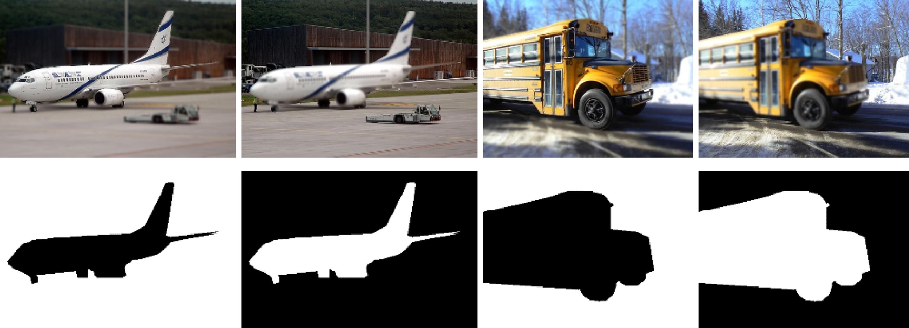
Training images and corresponding label images. (The first row are the multi-focus training images; the second row are the corresponding label images, which the black area pixels are 0 and the white area pixels are 1, marking the focused and unfocused areas of the source images respectively.

5.2 Experimental parameter setting

The experiments are implemented on the TensorFlow framework. During the training phase of the network, we use Xavier initialization [41] method to initialize all convolution kernel parameters except for the convolutional layers that migrated from the VGG-19 network. The RMSprop [42] optimizer is used to train our network. Initial learning rate is set as 1e-6; weight decay and momentum are respectively set as 0.001 and 0.9, and the finalized network model is obtained after 50 epochs of training.

5.3 Parametric ablation experiment

To verify the influence of the key parameters on the proposed method, we carried out some comparative experiments. We use a single cross entropy loss function to replace the layer-by-layer hybrid loss function, and name the network as Compare-loss. Based on the original network, we removed the BN layer, and named the new network as Compare-bn. We also changed the initialization mode of the convolutional layer in the network from Xavier to normal initialization, and named this network as Compare-initial. We trained these three networks to get the experimental results respectively. The comparison results are shown in the Table 1, the ablation experiments of these key parameters show that the final model of our proposed method achieves best results each metric.

Table 1
Comparison of parametric ablation experiments

Table 1 Q ^SF Q ^ABF Q ^LABF Q ^MI Q ^AG

Compare-loss 24.1453 0.756 0.2175 7.9003 11.2459

Compare-bn 23.9151 0.7272 0.2327 7.4178 11.0755

Compare-initial 24.1692 0.7562 0.2173 7.9035 11.2846

OURS 24.2697 0.7572 0.2166 7.9046 11.3021

Table 1	Q ^SF	Q ^ABF	Q ^LABF	Q ^MI	Q ^AG
Compare-loss	24.1453	0.756	0.2175	7.9003	11.2459
Compare-bn	23.9151	0.7272	0.2327	7.4178	11.0755
Compare-initial	24.1692	0.7562	0.2173	7.9035	11.2846
OURS	24.2697	0.7572	0.2166	7.9046	11.3021

5.4 Model stability analysis

To get an available model, we carried out a large number of experiments to verify the performance of the proposed model. We performed several experiments to verify the stability of our proposed method. In this sub-section, we retrain our neural network another four times to get four image fusion models, and the testing results of these models are shown in Table 2 and Fig. 8.

Table 2
The quality metrics after five experiments

Table 2 Q ^SF Q ^ABF Q ^LABF Q ^MI Q ^AG

Test 0 (final model) 20.8152 0.7634 0.2087 8.4095 8.2548

Test1 20.7977 0.7629 0.2098 8.4158 8.2485

Test2 20.7981 0.7634 0.21 8.434 8.2436

Test3 20.8023 0.7628 0.2094 8.4055 8.2508

Test4 20.8126 0.7622 0.2097 8.4005 8.2518

Table 2	Q ^SF	Q ^ABF	Q ^LABF	Q ^MI	Q ^AG
Test 0 (final model)	20.8152	0.7634	0.2087	8.4095	8.2548
Test1	20.7977	0.7629	0.2098	8.4158	8.2485
Test2	20.7981	0.7634	0.21	8.434	8.2436
Test3	20.8023	0.7628	0.2094	8.4055	8.2508
Test4	20.8126	0.7622	0.2097	8.4005	8.2518

As shown in Fig. 8, we cannot distinguish the difference among the experimental results of the five image fusion models, subjectively. We can find that the stability of our model is satisfactory, visually. In Table 2, we can see that the difference among the evaluation indicators obtained from the five experiments is very small, which shows the stability of the model proposed in terms of objective indicator.

Fig. 8

Model stability verification.

5.5 Experiments of TL-based method and non-TL-based method

To further verify the effectiveness of TL-based method, we also train a non-TL-based network whose structure was the same as the TL-based method for color multi-focus image fusion, and the experiments are shown in Fig. 9 and Table 3.

Fig. 9

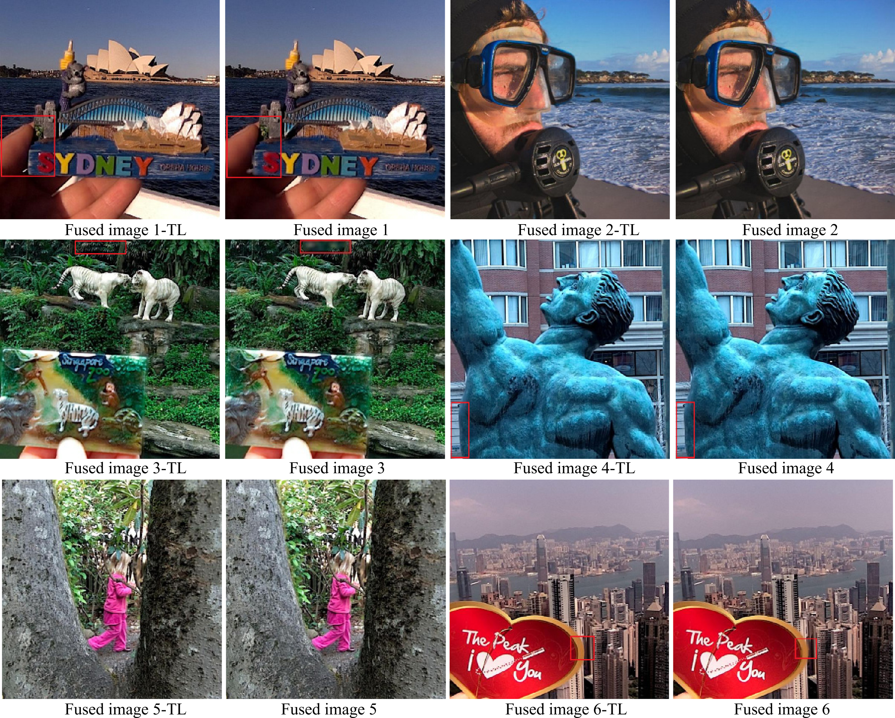
Comparison of TL-based method and our non-TL-based method.

Table 3

The quality metrics of TL-based method and our non-TL-based method

Table 2	Q ^SF	Q ^ABF	Q ^LABF	Q ^MI	Q ^AG
Fused image 1-TL	20.8152	0.7634	0.2087	8.4095	8.2548
Fused image 1	20.7142	0.7495	0.2181	8.3	8.1925
Fused image 2-TL	14.3223	0.7445	0.2419	9.0216	6.0664
Fused image 2	14.2243	0.7233	0.2427	8.8824	5.9927
Fused image 3-TL	28.0069	0.7898	0.1729	6.0176	14.5919
Fused image 3	27.7587	0.7793	0.1823	5.934	14.4243
Fused image 4-TL	26.6145	0.77	0.2017	7.9644	11.8953
Fused image 4	26.1047	0.7586	0.2143	8.0482	11.6378
Fused image 5-TL	32.0792	0.7422	0.2337	7.3856	17.5476
Fused image 5	32.0682	0.7419	0.2338	7.363	17.5327
Fused image 6-TL	23.9394	0.7332	0.2409	8.6287	9.5013
Fused image 6	23.8994	0.7217	0.2419	9.4013	9.4013

In the red boxes marked in Fig. 9, some blurred areas appear in the fused images obtained by the non- TL-based method. However, the fused images obtained by the TL-based method performs well without artifacts or blurred areas. The results show that the proposed TL-based method can achieve better performance compared with non-TL-based model. The evaluation metrics are listed in Table 3. The values of Q^ABF, Q^MI, and Q^AG of the TL-based method are better than those of the non-TL-based method.

The Q^SF values of the TL-based method are better than that by the non-TL-based method, except the fifth image pair. Besides, the Q^LABF value of the TL-based method are better than that of the non-TL-based method. In general, the metrics of the fused images obtained by the TL-based method are better than those by the non-TL-based method.

5.6 Comparison experiments with different methods

To demonstrate the effectiveness of the proposed method, several popular image fusion methods are contrasted with the proposed method, including ASR [26], CSR [27], DWT [40], MSVD [28], GD [38] MSTSR [29], MGIVF [30], PCA [40] IFCNN [46], SESF [45] and NEMI [32]. Moreover, the “Lytro” [39] dataset is employed to indicate the performance of different image fusion methods, and it is a commonly used dataset for multi-focus image fusion.

Five commonly used objective evaluation metrics are employed to evaluate the quality of fused images of different fusion methods, such as spatial frequency (Q^SF), edge feature similarity (Q^ABF), overall in formation loss (Q^LABF), mutual information (Q^MI) and average gradient (Q^AG). Among them, for the Q^LABF values, the smaller is better; for the other metrics, the larger values indicate the better quality of fused images.

The expression of Q^SFis as follows: $Q^{SF} = \sqrt{{RF}^{2} + {CF}^{2}}$ (9) $RF = \sqrt{\frac{1}{MN} \sum_{i}^{M} \sum_{j}^{N} (I (i, j) - I (i, j - 1))^{2}}$ (10) $CF = \sqrt{\frac{1}{MN} \sum_{i}^{M} \sum_{j}^{N} (I (i, j) - I (i - 1, j))^{2}}$ (11) where M and N are the width and height of the image respectively, I (i, j) is the pixel value of the image at position (i, j).

Q^ABF is an evaluation metric based on the richness of edge information and presented is as follows: $Q^{AF} (i, j) = Q_{δ}^{AF} (i, j) * Q_{σ}^{AF} (i, j)$ (12) $Q^{ABF} = \frac{\sum_{i}^{N} \sum_{j}^{M} (Q^{AF} W^{A} (i, j) + Q^{BF} W^{B} (i, j))}{\sum_{i}^{N} \sum_{j}^{M} (W^{A} (i, j) + W^{B} (i, j))}$ (13) where Q^AF represents the edge strength, $Q_{δ}^{AF} (i, j)$ and $Q_{σ}^{AF} (i, j)$ are the orientation preservation values of the region (i,j). W^A (i, j) and W^B (i, j) represent the weight coefficients of each image edge.

Q^LABF can be used to present the feature loss of the fused image and is expressed as follows: $Q^{LABF} = \frac{\sum_{i}^{N} \sum_{j}^{M} r_{N, M}}{\sum_{i}^{N} \sum_{j}^{M} (W^{A} (i, j) + W^{B} (i, j))}$ (14)

Q^MI is a measure of the interdependence between variables, and its expression is as follows: $Q^{MI} = \frac{{JE}_{A, F} + {JE}_{B, F}}{{IE}_{A} + {IE}_{B}}$ (15) where A and B respectively present two source images, and F represents the fused image, and JE_A,F and JE_B,F are the joint entropy between A, B and F, and IE_A and IE_B represent the information entropy of A and B respectively. Q^AG presents the gradient information of the fused image, as follow: $Q^{AG} = \frac{\sum_{i}^{M} \sum_{j}^{N} \sqrt{\frac{I (i + 1, j) - I (i, j)^{2} + I (i, j + 1) - I (i, j)^{2}}{2}}}{(M - 1) (N - 1)}$ (16)

Figure 10 shows the fused results of the first image pair, it can be seen that the color distortion of the fused images obtained by DWT and GD methods is relatively obvious than that of the fused images produced by other methods, and this phenomenon slightly exists in the fused image obtained by ASR. The loss of texture information of the fused images obtained by MVSD and PCA methods is serious, so that the visual quality of their whole images is poor. Some details of the fused images obtained by MGIVF and NEMI methods are missing, for example, the upper edge of the head of koala (as marked by the red box in Fig. 10) are obviously fuzzy. The quality of fused image obtained by CSR, and the proposed method is superior to that of other methods. In Fig. 11, the texture and detail of the fused images generated by MVSD and PCA methods are obviously lost, which can also be found in Fig. 12. Besides,

Fig. 10

The first group of fused images.

Fig. 11

The second group of fused images.

Fig. 12

The third group of fused images.

Figure 11 also reveals some detail loss in the fused images obtained by GD and NEMI. In Figs. 13 and 14, the fused image obtained by DWT method is obviously dark compared with that by other methods. In Fig. 14, the fused images obtained by PCA, MSVD and GD have the phenomenon of detail loss and edge blur, while DWT and MGIVF have color distortion.

Fig. 13

The fourth group of fused images.

Fig. 14

The five group of fused images.

Generally, the proposed method has the better performance on image details and edges without the problem of significant artifacts or ambiguous areas in the fused image, which indicates that the performance of the proposed method is better than most of other comparison methods visually.

However, because of the uncertainty and subjectivity of human vision, the images quality obtained by some methods is difficult to be distinguished visually. Therefore, various evaluation indexes are employed to verify and analyze the performance of different methods from objective perspective.

The objective evaluation metrics of different fused images are shown in Tables 4–9. In Tables 4, 5, 6, and 9, the Q^SF values obtained by proposed method is better than others, and the Q^ABF value obtained by our method is better and closer to IFCNN and SESF methods, and the Q^LABF value obtained by the SESF method is better than other methods and our method is the second. Besides, the Q^MI value of the proposed method are most similar to NMEI method and generally better than other methods. It can be seen from Tables 4, 5, 6 and 8 that the metrics obtained by the proposed method are superior to that by other methods except the Q^LABF. Besides, the Q^ABF and Q^AG values of the proposed method in Table 4 are far superior to that by other methods and close to the IFCNN and SESF. The Q^MI value is slightly lower than that of fused image obtained by NMEI, and the Q^LABF value is lower than SESF in Table 9, but other metrics obtained by the proposed method are better than those of other methods. In Table 8, the Q^MI value obtained by the proposed method is much better than other methods. According to above analysis, it can be found that the performance of the proposed method is generally better than most image fusion methods in objective evaluation metrics.

Table 4

The quality metrics of the first group of fused images

Table 3	Q ^SF	Q ^ABF	Q ^LABF	Q ^MI	Q ^AG
ASR [26]	19.2255	0.7232	0.2478	6.5245	7.7341
CSR [27]	19.3169	0.7048	0.2639	6.5513	7.591
DWT [40]	17.3321	0.6628	0.2991	5.9049	7.1369
MSVD [28]	16.9884	0.4721	0.4931	6.0726	6.9686
GD [40]	15.8638	0.6152	0.3608	5.8748	6.5651
MSTSR [29]	19.5494	0.7339	0.2372	6.8437	7.8577
MGIVF [30]	16.3579	0.6094	0.3543	5.7111	6.5657
PCA [40]	11.9602	0.4541	0.5261	6.4498	4.9552
NMEI [32]	20.0758	0.7361	0.2443	8.2753	7.843
IFCNN [46]	20.7156	0.7319	0.1895	6.9164	8.2486
SESF [45]	20.74	0.7611	0.2097	8.2324	8.2167
OURS	20.8152	0.7634	0.2087	8.4095	8.2548

Table 5

The quality metrics of the second group of fused images

Table 4	Q ^SF	Q ^ABF	Q ^LABF	Q ^MI	Q ^AG
ASR [26]	14.533	0.6938	0.2756	7.2641	5.2997
CSR [27]	14.4384	0.6833	0.2849	7.3052	5.1971
DWT [40]	12.6487	0.6104	0.3511	6.4957	4.7794
MSVD [28]	12.6194	0.5415	0.417	6.9204	4.7436
GD [38]	12.1812	0.6121	0.3613	6.4978	4.5776
MSTSR [29]	14.6239	0.7033	0.2682	7.5013	5.3682
MGIVF [30]	12.4728	0.595	0.3522	6.3314	4.6354
PCA [40]	9.7721	0.5316	0.4393	7.1247	3.807
NMEI [32]	14.158	0.744	0.2465	8.9776	5.9876
IFCNN [46]	14.4092	0.7143	0.1889	7.2533	6.1154
SESF [45]	14.3498	0.7416	0.2418	8.8282	6.0659
OURS	14.6323	0.7445	0.2419	9.0216	6.0216

Table 6

The quality metrics of the third group of fused images

Table 5	Q ^SF	Q ^ABF	Q ^LABF	Q ^MI	Q ^AG
ASR [26]	26.4299	0.7604	0.2061	4.3023	13.856
CSR [27]	25.7431	0.7482	0.2244	4.1658	13.4566
DWT [40]	22.3318	0.6491	0.3191	3.4495	11.8458
MSVD [28]	22.4159	0.5296	0.4289	3.6648	11.6142
GD [38]	22.492	0.6746	0.306	3.6515	11.8989
MSTSR [29]	27.0739	0.7781	0.1909	5.0103	14.1557
MGIVF [30]	22.2566	0.6384	0.3256	3.5294	11.6078
PCA [40]	16.9294	0.46	0.5254	3.7849	9.0291
NMEI [32]	27.6463	0.7806	0.1869	5.9606	14.3441
IFCNN [46]	27.645	0.762	0.1623	4.5563	14.4267
SESF [45]	27.9136	0.7851	0.1751	5.8004	14.5623
OURS	28.0069	0.7898	0.1729	6.0176	14.5919

Table 7

The quality metrics of the fourth group of fused images

Table 6	Q ^SF	Q ^ABF	Q ^LABF	Q ^MI	Q ^AG
ASR [26]	25.1657	0.7559	0.2132	6.538	11.4185
CSR [27]	25.6262	0.7577	0.2109	6.723	6.723
DWT [40]	22.0357	0.7103	0.2621	5.6215	10.2362
MSVD [28]	23.3204	0.6994	0.258	6.0798	10.7526
GD [38]	20.7827	0.6751	0.3052	5.1706	9.6396
MSTSR [29]	24.3735	0.7504	0.224	6.3678	11.1296
MGIVF [30]	21.692	0.6818	0.2874	5.5941	9.5225
PCA [40]	19.0789	0.6733	0.3014	6.2101	8.6719
NMEI [32]	25.8694	0.7633	0.2154	8.0634	11.5243
IFCNN [46]	26.9399	0.7518	0.1425	6.5585	12.0813
SESF [45]	26.6901	0.7689	0.2004	7.863	11.9929
OURS	26.145	0.77	0.2017	7.9644	11.8953

Table 8

The quality metrics of the five group of fused images

Table 7	Q ^SF	Q ^ABF	Q ^LABF	Q ^MI	Q ^AG
ASR [26]	30.2381	0.7319	0.7319	5.39	16.64
CSR [27]	30.6859	0.7317	0.2427	5.4066	16.8069
DWT [40]	25.7939	0.6796	0.3069	4.5368	14.2774
MSVD [28]	25.7513	0.4938	0.472	4.1441	13.5948
GD [38]	24.5506	0.6751	0.3416	4.2803	9.6396
MSTSR [29]	29.6478	0.7289	0.2564	5.3099	16.333
MGIVF [30]	25.2506	0.6277	0.3428	4.3745	13.4922
PCA [40]	22.1167	0.6086	0.3747	4.6606	12.4343
NMEI [32]	31.649	0.7384	0.2415	7.3224	17.2858
IFCNN [46]	32.1776	0.7275	0.1915	5.5704	17.7238
SESF [45]	31.9671	0.7325	0.2358	6.8523	17.3839
OURS	32.0792	0.7422	0.2337	7.3856	17.5476

Table 9

The quality metrics of the sixth group of fused images

Table 8	Q ^SF	Q ^ABF	Q ^LABF	Q ^MI	Q ^AG
ASR [26]	22.1237	0.7081	0.2683	6.7117	8.9273
CSR [27]	22.4245	0.6927	0.2809	6.7229	8.8266
DWT [40]	21.3293	0.6591	0.2942	5.7757	8.7025
MSVD [28]	18.1461	0.5803	0.3857	6.1167	7.5231
GD [38]	18.8461	0.6351	0.3432	5.8972	7.7836
MSTSR [29]	22.1615	0.7081	0.2683	6.7634	8.944
MGIVF [30]	18.4361	0.591	0.3724	5.6112	7.4242
PCA [40]	14.7626	0.5192	0.4561	6.0982	6.1865
NMEI [32]	23.7259	0.7325	0.246	8.629	9.3987
IFCNN [46]	23.7247	0.7008	0.2265	6.6018	9.4811
SESF [45]	23.7967	0.73	0.2438	8.5316	9.4651
OURS	23.9394	0.7332	0.2409	8.6287	9.5013

More experiments of the proposed method are shown in Fig. 16, in which we can find the focused areas of source images are effectively extracted and fused into the final images. In summary, the proposed method can achieve good performance in color multi-focus image fusion. Besides, the fused images have superior visual quality compared with those of other methods and have better performance in objective evaluation indexes as well. This experiment shows that the TL-based image fusion method is feasible and effective.

Fig. 15

The sixth group of fused images.

Fig. 16

More fused images obtained by the proposed method. (The first and second column are the multi-focus source images, and the third column are the fused images).

In summary, the proposed method can achieve good performance in color multi-focus image fusion. Besides, the fused images of the proposed method have superior visual quality compared with those of other methods and have better performance in objective evaluation indexes as well.

6 Conclusion

This paper proposes a color multi-focus image fusion method based on transfer learning. First, the trained VGG-19 was used to extract the primary features of the source images, and then an efficient network was designed based on the convolutional layer parameters transferred from the VGG-19 network, so that the image features are extracted again based on the newly designed network. Second, the primary decision mask is obtained by inputting the extracted deep features into the reconstruction network. Finally, an effective fusion strategy was designed to synthesize the fusion decision masks and generated the fused image. The experiments show that the proposed method is competitive. This work shows that the image fusion method based on transfer learning is feasible.

Based on the trained VGG-19 model, this paper realizes the transferring and reusing of the structures and parameters of VGG-19 network, which is combined with the newly designed model to achieve feature extraction of the source images. Given the advantages of TL, we will introduce TL to complete other image fusion tasks in future studies, such as remote sensing image fusion and medical image fusion.

Footnotes

Acknowledgments

This research was funded by the National Natural Science Foundation of China (Nos. 62101481, 62002313, 62066049), Key Areas Research Program of Yunnan Province in China (202001BB050076), Key Laboratory in Software Engineering of Yunnan Province in China (2020SE408).

References

Zhu

Z.Q.

, Qin

G.Q.

, et al., A Novel Multi-Focus Image Fusion Method Based on Stochastic Coordinate Coding and Local Density Peaks Clustering, Future Internet 8(4) (2016), 1–18.

G.Q.

, Zhu

, Zeng

F.C.

, et al., Multi-focus image fusion via morphological similarity-based dictionary construction and sparse representation, CAAI Transactions on Intelligence Technology 2(3) (2018), 83–94.

Liu

S.Q.

, Ma

, Yin

, et al., Multi-Focus Color Image Fusion Algorithm Based on Super Resolution Reconstruction and Focused Area Detection, IEEE ACCESS 8 (2020), 90760–90778.

Kou

, Zhang

L.G.

, Zhang

, et al., A multi-focus image fusion method via region mosaicking on Laplacian pyramids, PLOS One 161 (2019), 111–123.

Xiao

, Xu

B.C.

, Bi

X.L.

, et al., Global-Feature Encoding U-Net (GEU-Net) for Multi-Focus Image Fusion, IEEE Transactions on Image Processing 37 (2021), 163–175.

Tan

Z.Y.

, Gao

, Li

X.H.

, et al., A Flexible Reference-Insensitive Spatiotemporal Fusion Model for Remote Sensing Images Using Conditional Generative Adversarial Network, IEEE Transactions on Geoscience and Remote Sensing, Early Access, 2021.

Sannen

and Brussel

H.V.

, A multilevel information fusion approach for visual quality inspection, Information Fusion 13(1) (2012), 48–59.

LeCun

, Boser

, Denker

J.S.

, et al., Backpropagation applied to handwritten zip code recognition, Neural Computation 1(4) (1989), 541–551.

Y.F.

and Yang

H.J.

, Optical microscopy with flexible axial capabilities using a vari-focus liquid lens, Journal of Microscopy 258(3) (2015), 212–222.

10.

Daniel

, Optimum Wavelet Based Homomorphic Medical Image Fusion Using Hybrid Genetic-Grey Wolf Optimization Algorithm, IEEE Sensors Journal 18(16) (2018), 6804–6811.

11.

Kumar

B.K.S.

, Image fusion based on pixel significance using cross bilateral filter, Signal Image and Video Processing 9(5) (2015), 1193–1204.

12.

Tian

and Chen

, Adaptive multi-focus image fusion using a wavelet based statistical sharpness measure, Signal Processing 92(9) (2012), 2137–2146.

13.

Kumar

B.K.S.

, Multifocus and multispectral image fusion based on pixel significance using discrete cosine harmonic wavelet transform, Signal Image Video Process 7(6) (2013), 1125–1143.

14.

Lewis

J.J.

, O’Callaghan

R.J.

, Nikolov

S.G.

, et al., Pixel- and region-based image fusion with complex wavelets, Information Fusion 8(2) (2007), 119–130.

15.

Nencini

, Garzelli

, Baronti

, et al., Remote sensing image fusion using the curvelet transform, Information Fusion 8(2) (2007), 143–156.

16.

Wang

, Ma

and Gu

, Multi-focus image fusion using PCNN, Pattern Reconition 43(6) (2010), 2003–2016.

17.

C.B.

and Gao

S.S.

, Image Segmentation-Based Multi-Focus Image Fusion Through Multi-Scale Convolutional Neural Network, IEEE ACCESS 5 (2017), 15750–15761.

18.

Tang

, Xiao

, Li

W.S.

, et al., Pixel convolutional neural network for multi-focus image fusion, Information Science 433 (2018), 124–141.

19.

, Guo

, Lu

, et al., DRPL: Deep Regression Pair Learning for Multi-Focus Image Fusion, IEEE Transactions on Image Processing 29 (2020), 4816–4831.

20.

Liu

, Chen

and Rahardja

, A New Multi-Focus Image Fusion Algorithm and Its Efficient Implementation, IEEE Transactions on Circuits and Systems for Video Technology 30(5) (2020), 1374–1384.

21.

Jung

, Kim

, Jang

, et al., Unsupervised Deep Image Fusion with Structure Tensor Representations, IEEE Transitions on Image Processing 29 (2020), 3845–3858.

22.

H.G.

, Nie

R.C.

and Cao

J.D.

, Multi-Focus Image Fusion Using U-Shaped Networks With a Hybrid Objective, IEEE Sensor Journal 19(21) (2019), 9755–9765.

23.

Pan

S.J.

and Yang

, A Survey on Transfer Learning, IEEE Transactions on Knowledge and Data Engineering 22(10) (2010), 1345–1359.

24.

Simonyan

and Zisserman

, Very Deep Convolutional Networks for Large-Scale Image Recognition, arXiv preprint, arXiv: 1409.1556, 2014.

25.

Guo

X.P.

, Nie

R.C.

, Cao

J.D.

, et al., Fully Convolutional Network-Based Multifocus Image Fusion, Neural Computation 30(7) (2018), 1775–1800.

26.

Liu

and Wang

Z.F.

, Simultaneous image fusion and denoising with adaptive sparse representation, IET Image Processing 9(5) (2015), 347–357.

27.

Liu

, Chen

, Ward

R.K.

, et al., Image fusion with convolutional sparse representation, IEEE Signal Processing Letters 23(12) (2016), 1882–1886.

28.

Naidu

V.P.S.

, Image Fusion Technique using Multi-resolution Singular Value Decomposition, Defence Science Journal 61(5) (2011), 479–484.

29.

Liu

, Liu

S.P.

and Wang

Z.F.

, A general framework for image fusionbased on multi-scale transform and sparse representation, Information Fusion 24 (2015), 147–164.

30.

Bavirisetti

D.P.

, Xiao

, Zhao

J.H.

, et al., Multi-scale Guided Image and Video Fusion: A Fast and Efficient Approach, Circuits Systems and Signal Processing 38(12) (2019), 5576–5605.

31.

Audicana

M.G.

, Saleta

J.L.

, Catalan

R.G.

, et al., Fusion of multispectral and panchromatic images using improved IHS and PCA mergers based on wavelet decomposition, IEEE Transactions on Geoence and Remote Sensing 42(6) (2004), 1291–1299.

32.

Zhan

, Teng

J.C.

, Li

Q.Q.

, et al., A novel explicit multi-focus image fusion method,&, Multimedia Signal 6(3) (2015), 600–612.

33.

Weiss

, Khoshgoftaar

T.M.

and Wang

D.D.

, A survey of transfer learning, Journal of Big Data 3(1) (2016), 1–40.

34.

Zheng

Y.B.

, Teng

S.H.

, Liu

Z.Y.

, et al., Text Classification Based on Transfer Learning and Self-Training, Fourth International Conference on Neural Computation 3 (2008), 363–367.

35.

Meng

, Zhang

L.B.

, Gao

G.T.

, et al., Liver Fibrosis Classification Based on Transfer Learning and FCNet for Ultrasound Images, IEEE ACCESS 5 (2017), 5804–5810.

36.

Yang

J.H.

, Li

S.J.

and Xu

W.N.

, Active Learning for Visual Image Classification Method Based on Transfer Learning, IEEE ACCESS 6 (2018), 187–198.

37.

Peng

Y.F.

, Yan

S.K.

and Lu

Z.Y.

, Transfer Learning in Biomedical Natural Language Processing: An Evaluation of BERT and ELMo on Ten Benchmarking Datasets, SigbiomedWorkshop onBiomedicalNatural LanguageProcessing (BIONLP 2019), pp. 58–65, 2019.

38.

Paul

, Sevcenco

I.S.

and Agathoklis

, Multi-Exposure and Multi-Focus Image Fusion in gradient Domain, Journal of Circuits Systems and Computers 25(10) (2016).

39.

Lytro Multi-focus Dataset, Accessed: May 2016. [Online]. Available: http://mansournejati.ece.iut.ac.ir/content/lytro-multi-focus-dataset

40.

Oliver

, Pixel-level image fusion and the image fusion toolbox, DEC, 1990. [Online]. Available: http://www.metapix.de/toolbox.htm

41.

Glorot

and Bengio

, Understanding the difficulty of training deep feedforward neural networks, Journal of Machine Learning Research 9 (2010), 249–256.

42.

Hinton

, Lecture 6.5-RMSprop: Divide the gradient by a running average of its recent magnitude, COURSERA: Neural Networks for Machine Learning. [Online]. Available: http://www.cs.toronto.edu/ tijmen/csc321/slides/lectur slides lec6.pdf

43.

Misra

, Mish: A Self Regularized Non-Monotonic Neural Activation Function, https://arxiv.org/abs/1908.08681, 2019.

44.

Zhang

Z.Y.

, Xin

B.J.

, Deng

, et al., An investigation of ramie fiber cross-section image analysis methodology based on edge-enhanced image fusion, Measurement 145 (2019), 436–443.

45.

, Zhu

, Yin

, et al., SESF-Fuse: an unsupervised deep model for multi-focus image fusion, Neural Computing and Applications 33(11) (2021), 5793–5804.

46.

Zhang

, Liu

, Sun

, et al., IFCNN: A general image fusion framework based on convolutional neural network, Information Fusion 54 (2020), 99–118.

47.

Shi

, Sun

, Liu

, et al., Cloud-Based Data Offloading for Multi-focus and Multi-views Image Fusion in Mobile Applications, Mobile Networks and Applications 26 (2019), 830–841.

48.

Bhat

and Koundal.

, Multi-focus image fusion techniques: a survey, Artificial Intelligence Review 6 (2021), 1–53.

49.

Liu

, Wang

, Cheng

, et al., Multi-focus image fusion: A Survey of the state of the art, Information Fusion 64 (2020), 71–91.

50.

Huang

, Yang

, Jin

, et al., Multi-Sensor Image Fusion Using Optimized Support Vector Machine and Multiscale Weighted Principal Component Analysis, Electronics 9(9) (2020), 1531.

51.

Jiang

, Jin

, Chen

, et al., Two-scale decomposition-based multifocus image fusion framework combined with image morphology and Fuzzy Set Theory, Information Sciences 541 (2020), 442–472.

Color multi-focus image fusion based on transfer learning

Abstract

Keywords

1 Introduction

2 Related work

2.1 Convolutional neural network

3 The proposed method

3.1 Overall processes and framework

3.3.1 Feature reconstruction module

5.1 Production of training dataset

5.3 Parametric ablation experiment

Table 1 Comparison of parametric ablation experiments Table 1 Q SF Q ABF Q LABF Q MI Q AG Compare-loss 24.1453 0.756 0.2175 7.9003 11.2459 Compare-bn 23.9151 0.7272 0.2327 7.4178 11.0755 Compare-initial 24.1692 0.7562 0.2173 7.9035 11.2846 OURS 24.2697 0.7572 0.2166 7.9046 11.3021

Footnotes

Acknowledgments

References

Table 1
Comparison of parametric ablation experiments

Table 1 Q ^SF Q ^ABF Q ^LABF Q ^MI Q ^AG

Compare-loss 24.1453 0.756 0.2175 7.9003 11.2459

Compare-bn 23.9151 0.7272 0.2327 7.4178 11.0755

Compare-initial 24.1692 0.7562 0.2173 7.9035 11.2846

OURS 24.2697 0.7572 0.2166 7.9046 11.3021