Automatic phase identification of earthquake based on the UBDN deep network

Abstract

Seismic data obtained from seismic stations are the major source of the information used to forecast earthquakes. With the growth in the number of seismic stations, the size of the dataset has also increased. Traditionally, STA/LTA and AIC method have been applied to process seismic data. However, the enormous size of the dataset reduces accuracy and increases the rate of missed detection of the P and S wave phase when using these traditional methods. To tackle these issues, we introduce the novel U-net-Bidirectional Long-Term Memory Deep Network (UBDN) which can automatically and accurately identify the P and S wave phases from seismic data. The U-net based UBDN strongly maintains the U-net’s high accuracy in edge detection for extracting seismic phase features. Meanwhile, it also reduces the missed detection rate by applying the Bidirectional Long Short-Term Memory (Bi-LSTM) mode that processes timing signals to establish the relationship between seismic phase features. Experimental results using the Stanford University seismic dataset and data from the 2008 Wenchuan earthquake aftershock confirm that the proposed UBDN method is very accurate and has a lower rate of missed phase detection, outperforming solutions that adapt traditional methods by an order of magnitude in terms of error percentage.

Keywords

U-net bidirectional long short term memory phase identification wenchuan aftershocks

1 Introduction

Seismic phase identification is a solid foundation for earthquake prevention and disaster reduction work (e.g., earthquake early warning systems). Previously, manual identification and travel timetable-based calculations were the two main methods used to analyze various seismic phase data and identify seismic phases. In recent years, with the growth in the number of seismic stations, the amount of seismic data available has also increased significantly. The efficiency and accuracy of manual identification has therefore gradually decreased. At the same time, the noise pollution caused by urbanization leads to higher rates of missed detection of low-level earthquakes. Manual identification can no longer maintain the accuracy and efficiency of phase detection. Seismic phase automatic identification is thus becoming a more widely used approach [1]. It improves efficiency and reduces cost through faster processing of seismic data and higher identification rates.

Nowadays, seismic phase automatic detection is widely used to detect earthquakes. It utilizes characteristic equations, taking into account different parameters (e.g., amplitude and frequency). Thresholds are set based on these equations. Once a detected seismic phase reaches a preset threshold, the occurrence of an earthquake can be confirmed and its arrival time determined. Several methods are applied to seismic phase automatic identification. The Short-/Long-Term Average (STA/LTA) method uses the relationship between the average ratio of the short and the long time windows [2 –4], and the threshold value. The Akaike information criterion (AIC) method is used to find the best division point [5 –8] and the fractal dimension method then uses the fractal dimension value to determine the first arrival point [9 –13]. These methods are affected by environmental noise and have poor stability, resulting in low accuracy of identification and high rates of missed detection. In addition, the recognition results of these methods are significantly affected by the selection of features, functions, and parameters. The results often differ greatly from expectation when the signal-to-noise ratio (SNR) is low. Therefore, these methods are not efficient in seismic phase automatic identification when dealing with very large datasets.

Artificial intelligence and big data are now the most effective methods used to manage massive datasets [14]. Artificial neural networks have been developed and widely applied to the automatic identification of seismic phases because of their strong learning ability. The size of the dataset caused by the increasing number of seismic stations can therefore be addressed by applying neural networks. When handling massive datasets, an artificial neural network requires both training and converging data and the determination of related parameters (e.g., neurons; layers) through continuous experiment [15 –17]. To some extent, the application of neural networks to the automatic identification of seismic phases is limited due to the training processes required.

To address these limitations, a deep learning method has been developed for solving the neural network’s training difficulties [18]. In particular, the Convolutional Neural Network (CNN) approach to deep learning has been widely used in recent years. The CNN is classified according to multi-, shallow, and deep layers of convolutional structures. The multilayer convolution structure learns the features of the different levels, while the shallow layer learns the local features of the signal. Meanwhile, the deep convolutional layer is better at learning abstract features, which improves the classification and generalization capabilities of the CNN model compared to others. The deep convolutional layer structure of CNN is widely used in seismic signal noise reduction, seismic phase classification, and related matters [19]. Perol applied CNN to seismic phase identification [20] designing an eight-layer CNN with high identification accuracy. Ross manually annotated the dataset and used CNN for training [21]. Experimental results have shown that this trained CNN model has high identification accuracy. Meanwhile, the identification effect with low SNR and different regions is still within the ideal range. Yu Ziye input three-component seismic data into a 17-layer Inception model based on CNN after high-pass filtering [22]. At the same time, 100 datasets with different degrees of noise were added and tested. Their results proved that the deep learning method has a high tolerance for noise and is more stable than the AR-AIC+STA/LTA method. However, the above models based on CNN still have the problems of long training time and low computational efficiency.

Zhao Ming demonstrated that application of the U-net based model to seismic phase autoidentification has greatly improved the training speed [23], the accuracy of seismic phase identification, and the efficiency of dealing with the continuous waveform, all in comparison with STA/LTA. However, the U-net based training model still results in a 50%missed detection rate. The U-net is known for its efficient learning ability on two- or three-dimensional data. However, its high missed detection rate leads to poor learning ability for one-dimensional time series data (e.g., seismic data). In contrast, the use of Bidirectional Long Short-Term Memory (Bi-LSTM) in deep learning has proven to be efficient at processing the context of sequences and is more suitable for one-dimensional time series data. The application of Bi-LSTM to the identification and classification of heart sound signals of congenital heart disease by Zhu Lili and the pattern identification of quality control graphs by Wu Changliang have proved its efficiency with such data [24, 25].

To address the limitations in the application of U-net models to seismic phase autoidentification, we propose in this paper a novel U-net Bidirectional Long-Term Memory Deep Network (UBDN). This combines the advantages of U-net (e.g., fast training and accurate seismic phase identification) and Bi-LSTM (e.g., efficiency with one-dimensional time series data). The UBDN specifically maintains the accuracy of seismic phase identification. Based on that, a timing relationship can be established between seismic phase features. Seismic phase autodetection can therefore be achieved with high phase identification rates, low missed detection rates, and faster run times.

2 Methods

Taking the U-net as the framework, the structure of the UBDN model is shown in Fig. 1. The UBDN model uses the U-net to extract and learn the P and S wave phase characteristics in the seismic waveform data, and then utilizes Bi-LSTM to identify the P and S wave phases in the new seismic waveform.

Fig. 1

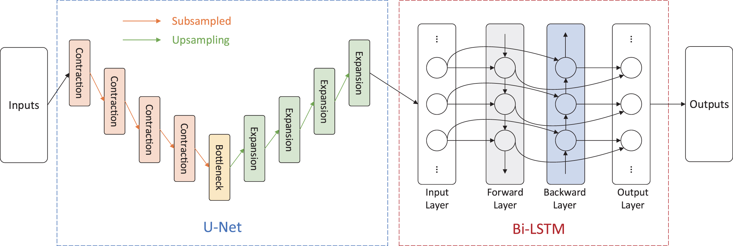
The UBDN model structure.

The input of the UBDN model is the original seismic waveform, and the output is marked with the P and S wave phases for the input. The blue dashed box contains the U-net component, and the red dashed box the Bi-LSTM network part. The U-net realizes the extraction of the features in the seismic waveform by determining the location of the P and S phases and finding the corresponding seismic points. The U-net model structure is shown in Fig. 2. Compared with the classic U-net, the network input was processed for dimensionality reduction. The input of the U-net defaults to two- or three-dimensional image data, and the seismic waveform data were one-dimensional time series data. Therefore, all inputs and outputs inside the network needed to be reduced to one dimension. The four subsampling layers on the left side performed convolution and pooling operations to extract the abstract features of the seismic phase; whereas the four upsampling layers on the right side completed operations such as transposed convolution and connection between the left and right symmetric layers. Recovering the detailed features of the seismic phases based on the learned features on the left side was conducive to solving the problem of seismic phase classification. Finally, the probability value of P wave, S wave, or noise was calculated by the activation function, and the category of the sampling point determined by comparing with the set threshold. At the same time, a loss function was used to adjust the hyperparameters such as the weight and bias of each layer to minimize the difference between the current network’s predicted value and the target value. The U-net consists of subsampling and upsampling layers. The subsampling layer comprises 2 one-dimensional convolutional layers and a pooling layer. In order to prevent overfitting, some dropout layers were randomly added. The upsampling layer consisted of a transposed convolutional, cropping, and convolutional layer. A dropout layer was again randomly added to prevent overfitting.

Fig. 2

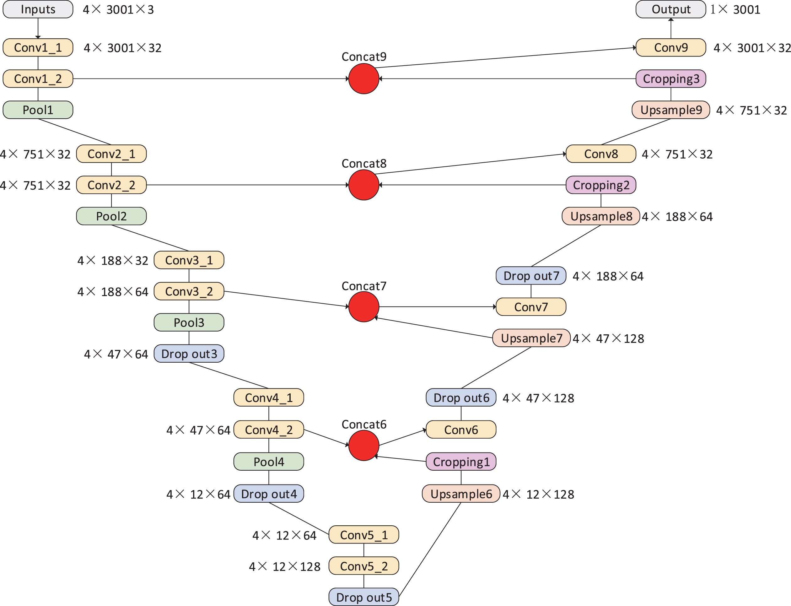
The U-net model structure.

The loss function used in this model is shown in Equation (1): $\begin{matrix} Loss = - \sum_{i = 1}^{3} \sum_{j = 1}^{n} Y_{ij}^{'} \cdot log (Y_{ij}) \end{matrix}$ (1)

In formula (1), Y′ is a label using binary coding; i = 1, 2, 3 respectively represent noise, P phase, and S phase; n is the number of waveform sampling points; and j = 1, …, n is the sampling point number. Y′ is shown in Equation (2): $Y_{i}^{'} = {\begin{matrix} Y_{1}^{'} : [1, 0, 0] \\ Y_{2}^{'} : [0, 1, 0] \\ Y_{3}^{'} : [0, 0, 1] \end{matrix}$ (2)

Y is the probability value calculated by the softmax function of the last layer, as shown in Equation (3): $\begin{matrix} Y_{i} = \frac{e^{z_{i}}}{\sum_{k = 1}^{3} e^{z_{k}}} \end{matrix}$ (3)

In Equation (3), z is the output tensor ([m, n, 3]) of the last layer, and m is the number of input data.

The Bi-LSTM network structure is shown in Fig. 3. The forward LSTM obtains a sequence h_a according to normal input. The backward LSTM reverses the input, and then passes it through a network with the same structure as the forward LSTM but with different weight parameters. Using this approach we eventually obtained a sequence which we then reversed to obtain h_b. Finally, we added the two sequences to get H, which is the final result through the Bi-LSTM network, as shown in Equation (4). $\begin{matrix} H = h_{a} \oplus h_{b} \end{matrix}$ (4)

Fig. 3

The Bi-LSTM model structure.

The network structure includes both a forward and a backward LSTM. The Bi-LSTM model can simultaneously utilize historical and future information in the sequence, divide the sequence information into two directions for input into the model, use two hidden layers to store the input information in both directions, and connect the corresponding outputs of the hidden layers to the same output layer. Both of them have the same structures and are independent of each other, and they only accept different sequence inputs. Therefore, the final hidden layer contains the positive and negative time series data for the dataset. Utilizing the advantages of Bi-LSTM in processing time series data, this establishes the timing relationship between seismic phase features, which solves the problem of missed detection caused by the use of the U-net in seismic phase identification.

3 Data and evaluation indicators

3.1 Data preprocessing

The UBDN model requires a large number of preset samples for training. The sample data used here came from the Stanford Earthquake Dataset (STEAD), which is sourced mainly from the International Seismological Center, the National Earthquake Information Center, the Northern California Seismic Network, the Southern California Seismic Network, the Pacific Northwest Seismic Network, The New Madrid Seismic Network, the Incorporated Research Institutions for Seismology, the Advanced National Seismic System Composite Catalog, and the Global Seismograph Network. The STEAD comprises data recorded by seismic stations around the world from January 1984 to August 2018 [26]. This article mainly selected seismic events of a magnitude between M0.5 and 2.5 with a SNR between 20 and 30 dB; the sampling rate was 100 Hz for sample data.

The sample data were preprocessed and the waveforms from 3 s before the arrival of the P wave to 10 s after the arrival of the S wave selected. We then uniformly cut the sample data to a length of 30 s (assigned a zero value if the length is insufficient), then normalized all the data as shown in Equation (5), where v_i represents the amplitude value of the seismic event signal, and data enhancement operations such as translation, noise addition, and filtering are adopted [27, 28] (Hayakawa et al. 1995; Schroff et al. 2015). $\begin{matrix} v_{i} = \frac{v_{i}}{\max | v_{i} |} \end{matrix}$ (5)

To ensure the quality of the dataset, it was manually cleaned and obvious labeling errors corrected. The final sample dataset consisted of 43,700 items, of which 80%were used as training data and 20%as testing data.

3.2 Evaluation index

In order to objectively evaluate the performance of the UBDN model in practical applications and ensure the reliability of the experimental results, we used the calculation of the root mean square error (RMSE), accuracy (A), and missed detection rate (M) of the different methods. The three formulas used to calculate these indicators were as follows: $\begin{matrix} RMSE = \sqrt{\frac{1}{n} \sum_{i = 1}^{n} [{(T_{i} - t_{i})}^{2}]} \end{matrix}$ (6)

$\begin{matrix} A = \frac{T_{e}}{(T_{e} + F_{e})} \end{matrix}$ (7)

$\begin{matrix} M = \frac{F_{n}}{(T_{e} + F_{n})} \end{matrix}$ (8)

RMSE denotes the root mean square error between the calculated time T_i of the model and the reference mark time t_i. This was used to reflect the accuracy of the pickup time of the model. n is the number of seismic events in the dataset; i is the serial number; A represents accuracy; T_e is the number of correct detections; and F_e the number of incorrect detections. The threshold for determining correctness was set as P±0.5 s, S±0.5 s and automatically picked up. The accuracy (A) of phase detection is the ratio of the number of phases for which the phase type is correct and within the error range identified by the model to the total number of phases. M represents the missed detection rate and F_n the number of missed seismic phases. M is computed as the ratio of the number of correct identifications to the number of manual identifications and used to check whether the model-identified seismic phase is complete relative to the reference phase, thus indicating the effectiveness of the model.

4 Experiments

Based on the UBDN model in Fig. 1, the experimental process framework design is shown in Fig. 4. Explain the complete experimental process of UBDN model training and testing. It comprised three main steps: ding172 Data preprocessing, where the original data were cut to a uniform length, and normalization and other pretreatment procedures carried out. At the same time, data enhancement operations such as translation, noise addition, and filtering were used to enhance the generalization ability of the model, and the preprocessed dataset divided into the training and testing datasets according to the 80:20 ratio given above. ding173 Model training, where the relevant dataset was used to train the UBDN model, the U-net to learn the seismic phase features, and the Bi-LSTM then used the features to complete the phase identification of the time series signal and output the seismic waveform data of the marked phase. ding174 Model evaluation and comparison, in which we used the output model to compare the pickup and reference times, and calculated the RMSE, accuracy (A) and missed detection rate (M) to evaluate the effectiveness of the model’s seismic phase identification.

Fig. 4

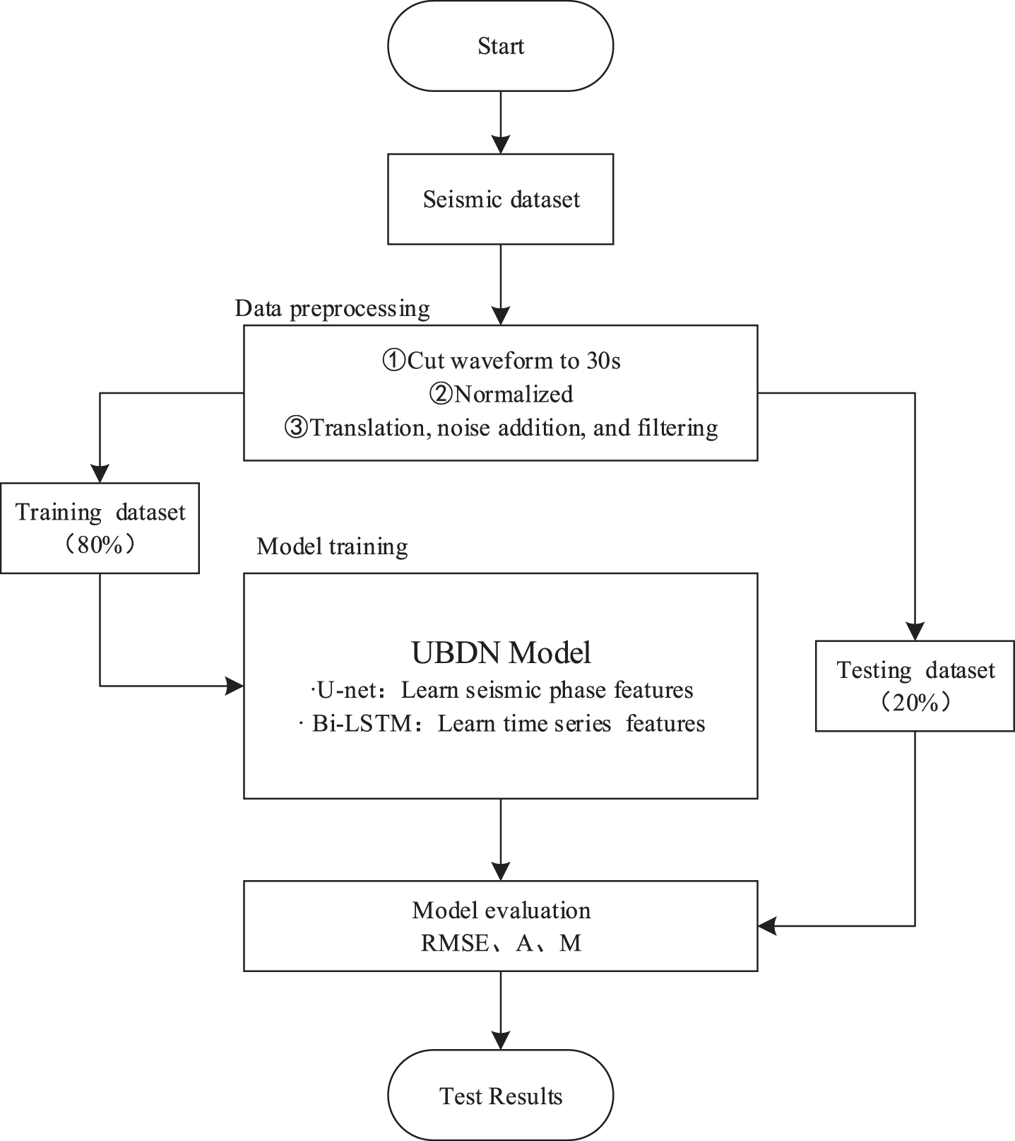
Experimental flowchart.

4.1 UBDN model training and testing

Firstly, the UBDN model was built and trained by Tensorflow and Keras before 80%(34,960 pieces) of waveform were selected as the training data, and 20%(8,740 pieces) as the testing dataset. The single training batch size was set to 32, the number of single training batches (n-input) to 100, and the number of earthquake events processed by a single training (n-step) set to 100. The UBDN model training used cross-entropy as the loss function and adopted the Adam algorithm to optimize the loss function calculation process. The Adam algorithm can speed up the convergence speed of the model because it has the advantages of high computational efficiency and adaptive learning rate. L2 regularization was used to prevent overfitting.

Figure 5 shows the training and testing results of the UBDN model. Figure 5(a) shows the training accuracy of the model; Fig. 5(b) shows the loss function value; Fig. 5(c) shows the phase identification Val Acc of the P wave on the testing dataset; and Fig. 5(d) shows the phase identification Val Acc of the S wave on the testing dataset. It can be seen from Fig. 5(a) and 5(b) that the UBDN model had an accuracy (A) of 98%after training the fourth cycle (about 20,000 time steps), and the loss value dropped to 0.03. The accuracy (A) and loss values of the following five cycles remained at this level, which shows that the UBDN model converged at this point after about 45,000 time steps. Figure 5(c) and 5(d) show that the accuracy (A) of the P and S wave phase identification on the testing dataset increased over time. From time steps 10,000 to 45,000, the P and S waves increased from 65.1%and 43.7%to 90.1%and 89.5%respectively. This indicates that the model did not overfit; furthermore, the longer the training time, the higher the accuracy. The experimental results in Fig. 5 show that the accuracy (A) of phase identification of P and S waves by the model was 90.1%and 89.5%, respectively, which meets the accuracy requirements for seismic phase identification. This indicates the model can be used effectively for this purpose.

Fig. 5

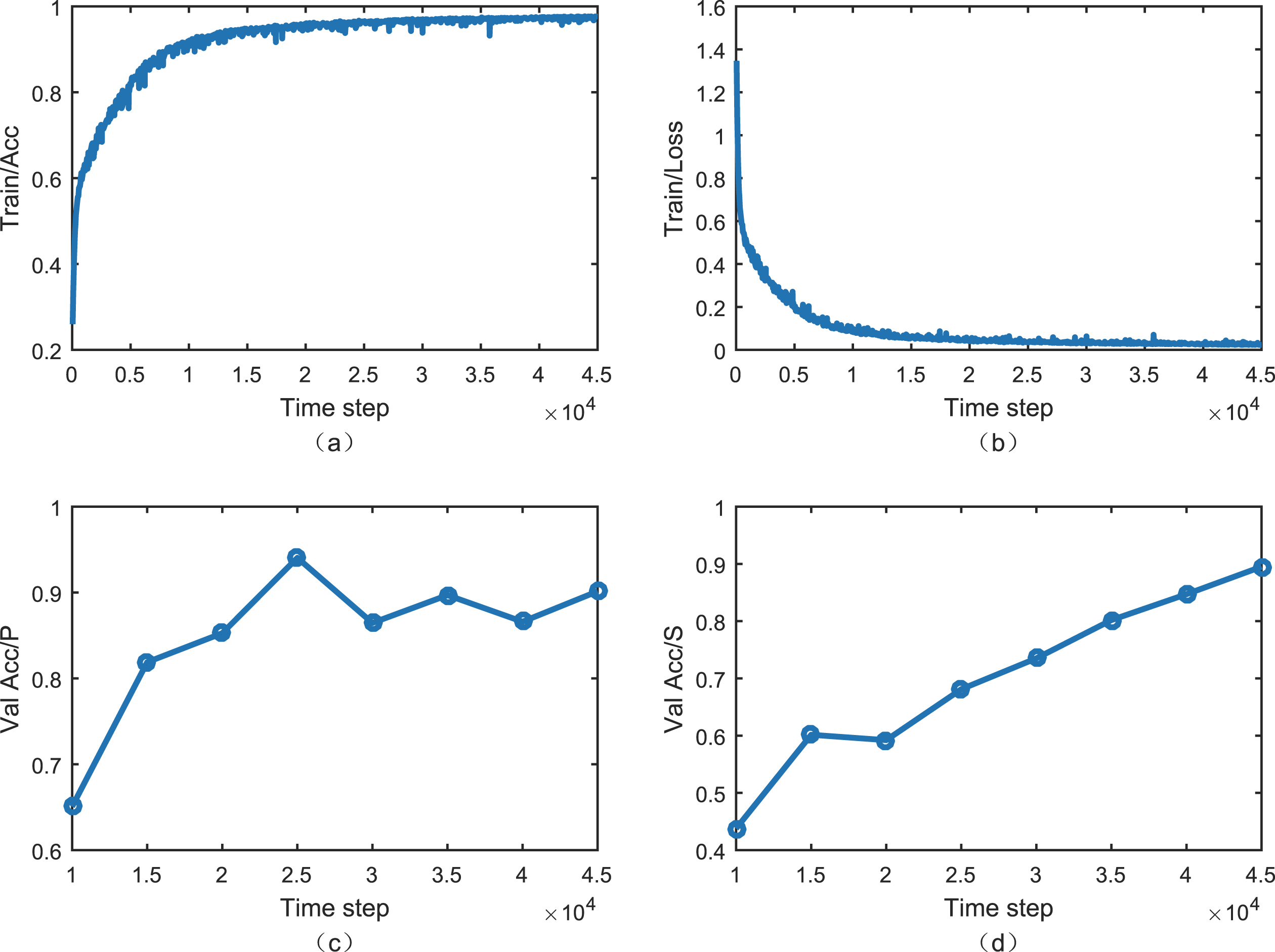
Training and testing process of the UBDN model.

4.2 Comparative experiments

In order to verify the seismic phase identification ability of the UBDN model, we compared it with the deep learning U-net (Zhao Ming et al. 2019), STA/LTA, and AIC seismic phase identification methods. In the comparative experiments, all models used a unified dataset of 2,000 pieces of waveform, and the SNR was concentrated between 20∼30 dB. We used formulas (6), (7), and (8) to calculate the RMSE, accuracy (A), and missed detection rate (M) so as to evaluate the detection results of the four models. The experimental results are shown in Table 1.

Table 1
Comparison of the UDBN model with the U-net, STA/LTA, and AIC methods

Method RMSE A M

UBDN P 0.26 87.99% 11.45%

S 0.27 87.60% 14.58%

U-net P 0.35 81.26% 30.74%

S 0.41 83.49% 28.40%

STA/LTA P 0.49 73.45% 37.52%

S 0.62 76.23% 35.87%

AIC P 0.43 75.13% 32.81%

S 0.58 78.92% 30.72%

Method	RMSE	A	M
UBDN	P	0.26	87.99%	11.45%
	S	0.27	87.60%	14.58%
U-net	P	0.35	81.26%	30.74%
	S	0.41	83.49%	28.40%
STA/LTA	P	0.49	73.45%	37.52%
	S	0.62	76.23%	35.87%
AIC	P	0.43	75.13%	32.81%
	S	0.58	78.92%	30.72%

As can be seen from Table 1, the RMSE of the UBDN model for the P and S waves was 0.26 s and 0.27 s, and the accuracy (A) was 87.99%and 87.61%. This represents a significant improvement over the traditional STA/LTA and AIC methods. The UBDN model also shows improvement in comparison with the U-net model. This indicates the UBDN model has obvious advantages compared with other methods in terms of accuracy. In terms of missed detection rates, the parameter M for the UBDN model was 11.45%and 14.58%. Compared with other methods, this is a significant reduction and indicates that the combination of the U-net and Bi-LSTM network approaches has achieved an ideal result in reducing the missed detection rate. The three evaluation indicators were highest for the UBDN model among the four methods tested.

Figure 6 shows the various possible scenarios for the UBDN model in the phase identification process. The black line shows when the P wave is picked up manually, and the red line when the S wave is picked up manually. Figure 6(a) shows the correct detection of the P and S wave phases; Fig. 6(b) the correct detection of the P-wave phase and the incorrect detection of the S-wave phase; Fig. 6(c) the correct detection of the S-wave phase and the incorrect detection of the P-wave phase; Fig. 6(d) the correct detection of the P-wave phase and missed detection of the S-wave phase.

Fig. 6

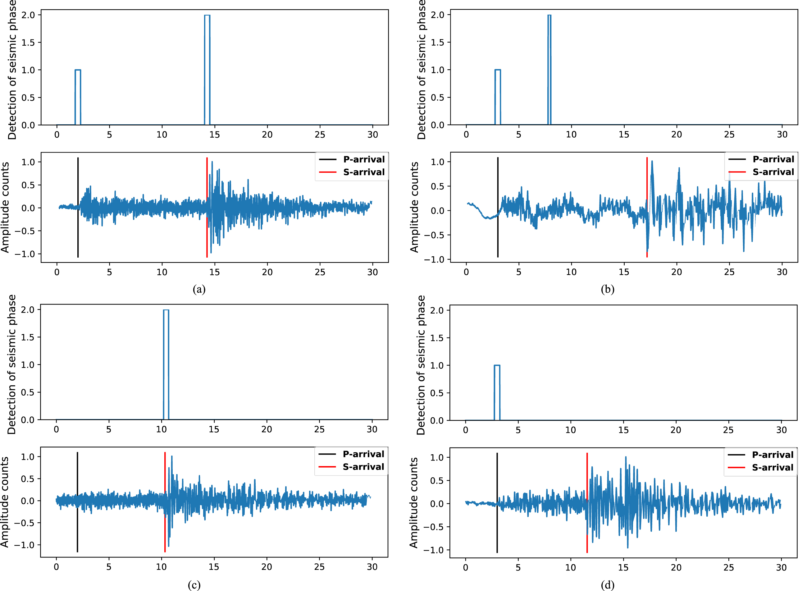
Different phase identification scenarios for the UBDN model.

4.3 Application of the model to the Wenchuan earthquake aftershocks

In order to verify the phase identification effect of the UBDN model in an actual earthquake event, it was applied to the aftershock dataset of the Wenchuan earthquake from May to September 2008. This dataset contains both seismic events and phase data. A total of 2,026 phase data items were collected from 76 stations. The SNR of the data was concentrated between 2∼5 dB, the sampling rate was 200 Hz, and the attribute fields included the earthquake time and longitude, latitude, depth, magnitude type, magnitude, reference location, event type, and so on (Data sharing infrastructure of national earthquake data center - http://data.earthquake.cn). An example event is shown in Fig. 7. This depicts the seismic events taking place at 14:53 on May 12, 2008. The magnitude is Ms6.3; the focal depth 14 km as recorded by the Maoxin Nanxin station (51MXN); the black line denotes the arrival of the manually picked P wave; and the red line the arrival of the manually picked S wave. Figure 7(a), 7(b), and 7(c) represent the vertical, north-south, and east-west seismic waveforms. The UBDN model was used to identify the phases of the Wenchuan earthquake aftershock dataset. The results are shown in Table 2.

Fig. 7

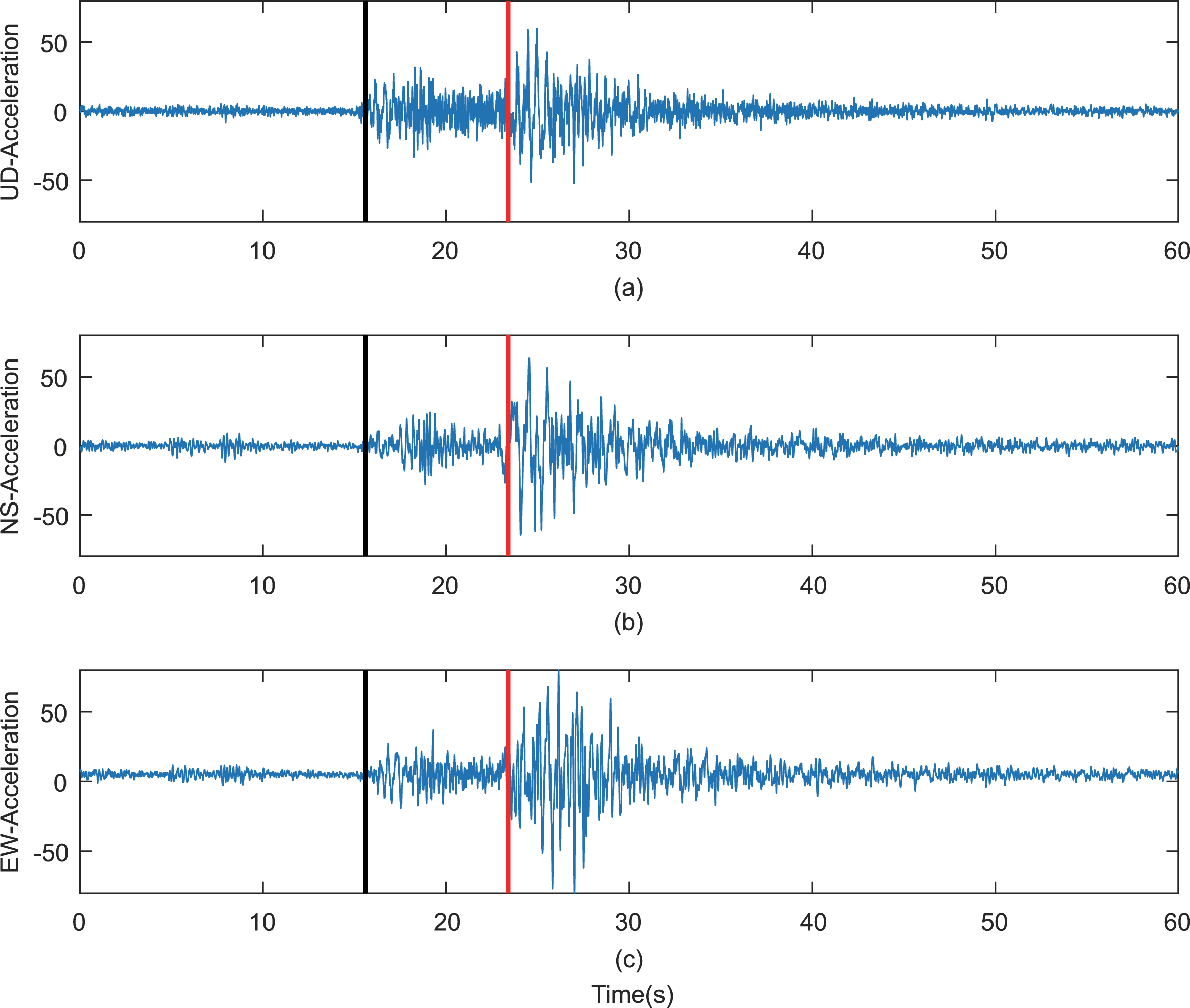
Examples of seismic event waveforms.

Table 2

Phase identification results for the UDBN model on the Wenchuan earthquake aftershock dataset

Method		RMSE	A	M
UBDN	P	0.31	80.69%	17.18%
	S	0.34	77.87%	20.56%

It can be seen from Table 2 that the RMSE of the UBDN model on the Wenchuan earthquake aftershock dataset was 0.31 s and 0.34 s, the accuracy (A) 80.69%and 77.87%, and the missed detection rate (M) 17.18%and 20.56%. Compared with the experimental results of the testing dataset, the effect of the UBDN model on the Wenchuan earthquake aftershock dataset is slightly poorer. This may be attributable to the different SNR of the datasets. To verify this hypothesis, the SNR of the aftershock dataset was concentrated in the range 2∼5 dB, and the SNR of the testing dataset in the range 20∼30 dB. Phase identification tests were then performed on five datasets with different SNR ranges of 0∼10 dB, 10∼20 dB, 20∼30 dB, 30∼40 dB, and >40 dB, with the number of events in each dataset set as 1,000.

The results of this experiment are shown in Fig. 8. It shows the accuracy (A), and missed detection rate (M) of the datasets with five different SNR ranges of 0–10, 10–20, 20–30, 30–40, >40(dB) on the UBDN model. It can be seen that the RMSE, accuracy (A), and missed detection rate (M) all have a linear relationship with SNR. As the SNR increases, RMSE and M gradually decrease, but A gradually rises. This indicates that the higher the SNR of the data, the better the seismic phase identification of the UBDN model. Although the effect for the actual Wenchuan earthquake aftershock dataset is slightly lower than that for the testing dataset, it can still meet the needs of practical applications. Therefore, the UBDN model has a certain degree of adaptability, and can still achieve a good seismic phase identification effect under the condition of low SNR.

Fig. 8

Phase identification results for datasets with different SNR.

5 Conclusion

Based on U-net and Bi-LSTM structures, we designed a UBDN seismic phase automatic identification model, used it to train a dataset, and established the relationship between the phase arrival time and the seismic waveform phase for real-time identification. By comparing the results of the trained model with those for other identification methods, and performing testing and experimental analysis using the 2008 Wenchuan earthquake aftershock dataset, we can draw the following conclusions. Firstly, the UBDN model can achieve sufficient accuracy to meet the requirements of seismic phase identification; secondly, compared with other methods, it offers a significant improvement on accuracy and a significant reduction in the missed detection rate; and thirdly, using the UBDN model with a real-life dataset (i.e., the Wenchuan earthquake aftershock data) shows that there is still a strong phase identification effect and further indicates that the model has good adaptability.

In practical applications, low-SNR data have an impact on the identification capabilities of the UBDN model. Future research may consider using seismic data collected by the same type of instrument and processed by the same noise reduction method as a dataset for model training, according to the noise level and sensitivity of seismic instruments and the difference in data noise reduction methods. This approach can greatly reduce the influence of SNR on the results of the UBDN model training and identification process and thus improve its stability.

Footnotes

Acknowledgments

This work was supported by the Special Fund of Teaching reform research and practice project (Grant No. 2019GJJG471), Basic scientific research projects of Central Universities (Grant No. ZY20180112), New engineering specialty reform projects (Grant No. E-SXWLHXLX20202607), 2020 education research and teaching reform project of College of disaster prevention and technology (Grant No. JY2020A12), The National Key Research and Development Programme of China (Grant No. 2018YFC1503801), and the Scientific Research Project Item of Hebei Province Education Department (Grant No. QN2018317).

References

D.P.

, Research on real time method of seismic phase identification. Dissertation, Institute of Engineering Mechanics, (2004).

Allen

R.V.

, Automatic earthquake recognition and timing from single traces[J], Bulletin of the Seismological Society of America 68(5) (1978), 1521–1532.

Baer

and Kradolfer

, An automatic phase picker for local and teleseismic events[J], Bulletin of the Seismological Society of America 77(4) (1987), 1437–1445.

Withers

, Aster

, Young

, Beiriger

, Harris

, Moore

and Trujillo

, A comparison of select trigger algorithms for automated global seismic phase and event detection, Bulletin of the Seismological Society of America 88(1) (1998), 95–106.

Akaike

, A new look at the statistical model identification, IEEE Transactions on Automatic Control 19(6) (1974), 716–723.

Sleeman

and Van Eck

, Robust automatic P-phase picking: an on-line implementation in the analysis of broadband seismogram recordings, Physics of the Earth and Planetary Interiors 113(1–4) (1998), 265–275.

Akazawa

, A technique for automatic detection of onset time of P-and S-phases in strong motion records, In Proc of the 13th World Conf on Earthquake Engineering. Vancouver, Canada, 1–6 August (2004).

Liu

J.S.

, Wang

and Yao

Z.X.

, On micro-seismic first arrival identification: A case study, Journal of Geophysics 56(5) (2013), 1660–1666.

Boschetti

, Dentith

M.D.

and List

R.D.

, A fractal-based algorithm for detecting first arrivals on seismic trances, Geophysics 61(4) (1996), 1095–1102.

10.

Chang

and Liu

Y.K.

, Generalized fractal dimension of seismic records and its application, Journal of Geophysics 2002(06) (2002), 839–846.

11.

Han

X.J.

, Shi

Z.J.

and Li

Y.L.

, An improved algorithm for picking up seismic first arrivals by using fractal dimension, Petroleum Geophysical EXploration 37(1) (2002), 60–63+98.

12.

Cao

M.S.

, Ren

Q.W.

, Wan

L.M.

and Luo

, Length fractal dimension method for picking seismic first break, Petroleum Geophysical Exploration 2004(05) (2004), 509–514+493–494+628.

13.

Tang

Y.L.

, The application of fractal theory in P-wave detection, Dissertation, Southwest Jiaotong University. (2017).

14.

Dai

and MacBeth

, The application of back-propagation neural network to automatic picking seismic arrivals from single-component recordings, Journal of Geophysical Research: Solid Earth 102(B7) (1997), 15105–15113.

15.

Zhang

F.M.

, Li

Q.H.

, Zhang

Y.S.

, Sheng

G.Y.

and Fan

, The seismic signal and phase recognition by using artificial neural network theory, Journal of Northwest Seismology 1998(04) (1998), 43–49.

16.

Wang

J.F.

and Luo

S.X.

, The improved bp neural network and its application in seismic first breaks picking, Calculation Technology of Geophysical and Geochemical Exploration 28(1) (2006), 14–17.

17.

Wang

and Chen

J.H.

, An automatic seismic event detection method based on artificial neural network, Seismogeomagnetic Observation and Research 29(3) (2008), 41–45.

18.

Ross

Z.E.

, Meier

M.A.

and Hauksson

, P wave arrival picking and first-motion polarity determination with deep learning, Journal of Geophysical Research: Solid Earth 123(6) (2018), 5120–5129.

19.

Zhao

, Chen

, Fang

L.H.

and Yuen

D.A.

, Earthquake phase arrival auto-picking based on U-shaped convolutional neural network, Journal of Geophysics 62(08) (2019), 3034–3042.

20.

Perol

, Gharbi

and Denolle

M.A.

, Convolutional neural network for earthquake detection and location, Science Advances 4(2) (2018).

21.

Ross

Z.E.

, Meier

M.A.

, Hauksson

and Heaton

T.H.

, Generalized seismic phase detection with deep learning, Bulletin of the Seismological Society of America 108(5A) (2018), 2894–2901.

22.

Z.Y.

, Chu

R.S.

and Sheng

M.H.

, Pick onset time of P and S phase by deep neural network, Journal of Geophysics 61(12) (2018), 4873–4886.

23.

Zhao

, Chen

and Yuen

, Waveform classification and seismic recognition by convolution neural network, Journal of Geophysics 62(1) (2019), 374–382.

24.

Zhu

L.L.

, Research on heart sound recognition of congenital heart disease based on Bi-LSTM network. Dissertation, Yunnan University. (2019).

25.

C.L.

, Zhu

, Wang

Y.W.

and Zhao

S.R.

, Quality Control Chart Pattern Recognition Based on Bidirectional LSTM, Software 40(07) (2019), 89–95.

26.

Mousavi

S.M.

, Sheng

, Zhu

, et al., Stanford Earthquake Dataset (STEAD): A global dataset of seismic signals for AI, IEEE Access: (2019), 179464–179476.

27.

Hayakawa

M.S.

, Effects of the chaotic noise on the performance of a neural network model for optimization problems, Physical review. E, Statistical physics, plasmas, fluids, and related interdisciplinary topics 51(4) (2693), R2693–R2696.

28.

Schroff

, Kalenichenko

and Philbin

, Facenet: A unified embedding for face recognition and clustering, Proceedings of the IEEE conference on computer vision and pattern recognition 2015 (2015), 815–823.

Automatic phase identification of earthquake based on the UBDN deep network

Abstract

Keywords

1 Introduction

2 Methods

3.1 Data preprocessing

Table 1 Comparison of the UDBN model with the U-net, STA/LTA, and AIC methods Method RMSE A M UBDN P 0.26 87.99% 11.45% S 0.27 87.60% 14.58% U-net P 0.35 81.26% 30.74% S 0.41 83.49% 28.40% STA/LTA P 0.49 73.45% 37.52% S 0.62 76.23% 35.87% AIC P 0.43 75.13% 32.81% S 0.58 78.92% 30.72%

Footnotes

Acknowledgments

References

Table 1
Comparison of the UDBN model with the U-net, STA/LTA, and AIC methods

Method RMSE A M

UBDN P 0.26 87.99% 11.45%

S 0.27 87.60% 14.58%

U-net P 0.35 81.26% 30.74%

S 0.41 83.49% 28.40%

STA/LTA P 0.49 73.45% 37.52%

S 0.62 76.23% 35.87%

AIC P 0.43 75.13% 32.81%

S 0.58 78.92% 30.72%