Joint decision-making model of preventive maintenance and delayed monitoring SPC based on imperialist competitive algorithm

Abstract

This paper develops a joint decision-making model approach to preventive maintenance and SPC (statistical process control) with delayed monitoring considered. The proposal of delayed monitoring policy postpones the sampling process till a scheduled time and contributes to six renewal scenarios of the production process, where maintenance actions are triggered by scheduled duration of preventive maintenance or the alert of $\bar{X}$ chart for monitoring the shift of process mean resulted by deterioration of equipment. By analyzing the evolution of the system in different scenarios, a mathematical model is given to minimize the expected cost per unit time by optimizing values of five variables (scheduled duration without monitoring, scheduled duration of preventive maintenance, sample size, sampling interval and control limit). The results of a numerical example indicate that the hourly cost of the proposed model is lower than the model that delayed monitoring is not considered when the system has a low hazard rate during the early period. Finally, a sensitivity analysis is performed to demonstrate the effect of model parameters.

Keywords

Repairable system delayed monitoring preventive maintenance statistical process control joint economic design

1 Introduction

Preventive maintenance (PM), which refers to a maintenance of a system performed at a planned time can reduce the occurrence of failures to maintain and ensure the reliability and availability of production process [1]. It has an important role in improving product quality and reducing production costs, as quality control policies and production planning do. Indeed, in many situations, the non-conforming items of production can be explained by a dysfunction or a failure of the production system [2]. Park [3] established an economic production model with the least expected cost, taking into account the defect rate of the manufacturing machine and PM, and demonstrated the close relationship between process quality control and maintenance. In addition, Wenzhu et al. [4] proposed an integrated decision model of production scheduling and PM. Furthermore, Bouslah et al. [5] developed a model by integrating maintenance policies and quality control with the Average Outgoing Quality Limit (AOQL) constraint. Lesage and Dehombreux [6] proposed a simulation model that enabled the joint optimization of PM and quality control policies. They indicated that integrated analysis performed better than the two stand-alone optimization. Therefore, the researches of integrated PM and SPC have attracted much attention in recent year.

As one of the two main tools of SPC, the control chart is popularly used to monitor production process to rapidly identify process quality shifts. In practice, the condition of the equipment has a direct effect on the quality of the products it makes, and it is the control chart that can signal the state of the equipment, so it is viewed as a trigger of the maintenance policy [7]. Thus, the joint economic design of control chart and maintenance has become the research theme of integrated PM and SPC. In this regard, Linderman et al. [8] are among the earliest researchers who performed a generalized analytic model that incorporates $\bar{X}$ chart and maintenance policy to minimize total expected cost. In the model, there were three renewal scenarios and maintenance actions which were triggered only by the true signal of control chart or scheduled time of PM. Some researchers extended this model to some other conditions. Zhou and Zhu [9] modified the model from three to four scenarios with the false alarm of the control chart to be considered. Whether Linderman model or Zhou and Zhu model, a quality shift caused by the deterioration of an equipment was taken into account, but the failure of an equipment was out of their considerations. On the issue, Mehrafrooz and Noorossana [10] extended the policy to six scenarios, where both the equipment failure and deterioration were assumed to cause quality shifts. Given that an equipment usually has a relatively low hazard rate during the preliminary period, H. Yin et al. [11] further developed a ten-scenario model by employing a delayed monitoring policy. In addition, Xiang [12] presented an integrated model of control chart and maintenance for a production system where equipment deterioration process was formulated as a discrete-time Markov chain. Liping Liu et al. [13] also proposed an integrated model of SPC and condition-based maintenance for a geometric process system. Panagiotidou and Nenes [14] developed an integrated model of adaptive variable-parameter (VP) Shewhart control chart and maintenance. Considering the unique complex characteristics of multi-stage process, Liu et al. [15] proposed an integrated model of $\bar{X}$ control chart and maintenance for two-unit series system. Also, other authors such as Zhong and Ma [16] conducted their studies on integrated control chart and maintenance for multi-stage system. Rasay et al. [17] presented an integrated model of SPC and maintenance planning for a two-stage dependent process under general deterioration.

For all the literatures mentioned above, the control chart integrated in the model is Shewhart $\bar{X}$ chart. Recently, a few researchers studied other control charts. Mehdi and Nidhal [18] studied an integrated maintenance and control policy based on quality control where the non-conforming units rate chart was used to identify the process condition. Yin and Makis [19] and Wang [20] employed a multivariate Bayesian control chart and a simulation-based multivariate Bayesian control chart for condition-based maintenance separately. Salmasnia et al. [21] proposed an integrated model that the VP T² Hotelling chart was used to monitor multiple quality characteristics. Yaping Li et al. [22] studied the joint economic design of CUSUM chart and age-based imperfect PM policy. In response to the condition of distribution-free, Khrueasom et al. [23] proposed an integrated decision model of PM and KS (Kolmogorov–Smirnov) control chart. For processes with small migration, Charongrattanasakul et al. [24] developed an integrated model of PM and Exponentially Weighted Moving Average (EWMA) control chart. He et al. [25] presented a reliability-oriented optimization model for joint PM and process quality control with time-between-events (TBE) control chart, where the impact of manufacturing process on product final reliability was considered to reduce the product reliability degradation originating from latent manufacturing defects.

In recent years, the research is further extended to the integration of quality, maintenance and production. Bouslah et al. [26] proposed a combined mathematics and simulation-based modeling framework to jointly optimize the production, quality and maintenance control settings for a two-machine line subject to operation-dependent and quality-dependent failures. Cheng et al. [27] considered an integrated problem of production lot sizing, quality control and condition-based maintenance for an imperfect production system subject to both reliability and quality degradations, and the aim of the model was to jointly optimize the lot size, the inventory threshold, the PM and overhaul thresholds so that the total cost per unit time was minimized. Salmasnia et al. [28] presented an integrated model for joint determination of production run length, adaptive control chart parameters and maintenance policy and the particle swarm optimization algorithm was used to minimize the total cost per production cycle subject to statistical quality constraints.

However, considering the relatively low hazard rate of equipment and quality shift during the initial production phase [29], the necessity of taking samples at an early age of the production process needs to be reconsidered. This paper attempts to develop a joint decision-making model approach of PM and $\bar{X}$ chart based on delayed monitoring. Different from the previous integrated model proposed by Yin H et al. [11], this paper contributes to six scenarios to describe the production system by analyzing each sampling interval and the introduction of delayed monitoring policy. In addition, same as other existing research results, reference 11 also established the renewal cost and renewal cycle model on the basis of expected cost and expected time of in-control and out-of-control process. Therefore, when analyzing the time and cost of out-of-control process, the Average Run Length (ARL) of the control chart was used. However, ARL represents the average out-of-control length under the condition of unlimited use. When considering the PM period T, the control chart actually operates under the condition of limited use period. That is, the influence of planned maintenance period T to operation time is ignored. Considering the limitation, we use the sampling interval as the basic analysis unit instead of the traditional two-stage analysis mode, and the in-control and out-of-control time of the system can be calculated by actual scenario measurement rather than ARL estimation, which do not neglect the impact of PM cycle T on the operation time. The object of the paper is to determine the five optimal variables (scheduled duration without monitoring, scheduled duration of PM, the sample size, sampling interval and control limit) to minimize the expected cost.

The remainder of this paper is organized as follows. Section 2 describes the assumption and notations. In Section 3, the evolution of the system and the cost function of the integrated model are analyzed in detail. In Section 4, the Imperialist Competitive Algorithm (ICA) is reported as a solution algorithm of the model, and a numerical example, the comparison analysis and sensitivity analysis are conducted. The conclusion is drawn and the further researches in the future are discussed in the last section.

2 Assumptions and notations

We consider a production system consisting of single equipment for single product with two states: good and deterioration. The system cannot generate deteriorating signal by itself, but the deterioration can cause shifts of process mean. For this reason, the process is monitored by using a $\bar{X}$ chart. Considering that the occurrence probability of equipment deterioration is low in the early stage, which results in a less possibility of process quality shift, the sampling process is postponed till a scheduled time to reduce the operation cost. Maintenance action is triggered by alert signal of the control chart or the scheduled time of PM. Therefore, the system must be shut down to inspect and repair if the control chart alarms before the scheduled time of PM, otherwise it keeps running to the scheduled time to perform PM. The system begins with a good state and is “as good as new” after a maintenance. All kinds of maintenance time and cost cannot be ignored. Table 1 describes the parameters used in this paper.

Table 1
Nomenclature

Parameter Description

f(u), F(u) pdf and cdf of the time of quality shift caused by deterioration of production system.

T ₁ average time to perform compensatory maintenance(CM).

T ₂ average time to perform reactive maintenance(RM).

T ₃ average time to perform preventive maintenance(PM).

Cm ₁ average cost to perform compensatory maintenance(CM).

Cm ₂ average cost to perform reactive maintenance(RM).

Cm ₃ average cost to perform preventive maintenance(PM).

Cl ₁ quality loss per unit time during in-control period.

Cl ₂ quality loss per unit time during out-of-control period.

Cd average shutdown loss per unit time.

u ₀ expected mean of process quality characteristic.

σ ₀ ² expected variance of process quality characteristic.

δ ₁ mean shift coefficient of process quality characteristic during out-of-control period.

T_d scheduled duration without monitoring (optimal variable).

T_p scheduled duration of preventive maintenance(PM) (optimal variable).

h sampling interval (optimal variable).

k control limit parameter (optimal variable).

n sample size (optimal variable).

C_f fixed cost per sampling.

Cq variable cost per sampling.

Cs total cost per sampling, Cs = n×C_q + C_f .

α probability of type I error.

β probability of type II error.

L maximum sampling number during scheduled duration of preventive maintenance (PM), L = [(T_p-T_d)/h].

Parameter	Description
f(u), F(u)	pdf and cdf of the time of quality shift caused by deterioration of production system.
T ₁	average time to perform compensatory maintenance(CM).
T ₂	average time to perform reactive maintenance(RM).
T ₃	average time to perform preventive maintenance(PM).
Cm ₁	average cost to perform compensatory maintenance(CM).
Cm ₂	average cost to perform reactive maintenance(RM).
Cm ₃	average cost to perform preventive maintenance(PM).
Cl ₁	quality loss per unit time during in-control period.
Cl ₂	quality loss per unit time during out-of-control period.
Cd	average shutdown loss per unit time.
u ₀	expected mean of process quality characteristic.
σ ₀ ²	expected variance of process quality characteristic.
δ ₁	mean shift coefficient of process quality characteristic during out-of-control period.
T_d	scheduled duration without monitoring (optimal variable).
T_p	scheduled duration of preventive maintenance(PM) (optimal variable).
h	sampling interval (optimal variable).
k	control limit parameter (optimal variable).
n	sample size (optimal variable).
C_f	fixed cost per sampling.
Cq	variable cost per sampling.
Cs	total cost per sampling, Cs = n×C_q + C_f .
α	probability of type I error.
β	probability of type II error.
L	maximum sampling number during scheduled duration of preventive maintenance (PM), L = [(T_p-T_d)/h].

3 Model development

3.1 System analysis

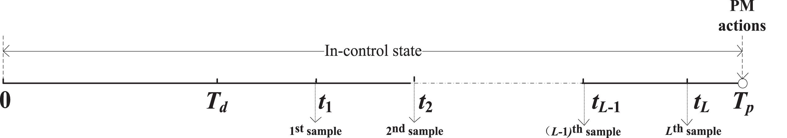
In light of the assumptions, the production process can be divided into three stages: delayed monitoring period, control chart monitoring period and maintenance period. As any maintenance makes system “as good as new”, the delayed monitoring policy and two types of errors of $\bar{X}$ chart can contribute to six renewal scenarios. The evolution course of the system is illustrated in Fig. 1.

Fig. 1

The evolution of the system.

In S₁-S₂, a system deterioration occurs during the delayed monitoring period and process quality shifts occur correspondingly. As the system cannot generate deteriorating signals by itself which has been assumed above, it still keeps running during the delayed monitoring period and inevitably enters the control chart monitoring period. Due to the type II error of control chart, the quality shift may be detected or may not be detected during monitoring period. If the control chart alarms (it is a true alert signal) during a sampling inspection, which means that the deterioration of the system is detected, the system will shut down immediately to perform reactive maintenance (RM), resulting in S₁. RM is a maintenance performed to respond to a break or a fault of a system. Generally, RM work such as replacement of parts is performed. If the control chart does not alarm (it makes type II error at every sampling), which means that the deterioration of system has not been detected during all the control chart monitoring period, the system will run to the scheduled time of PM. Since the system has already been out of control, the RM is still implemented, resulting in S₂.

In S₃-S₆, the system keeps good state and no corresponding quality shifts occur during the delayed monitoring period. After the system enters the control chart monitoring period, if a quality shift caused by the system deterioration occurs, the scenario is similar to S₁-S₂: if the deterioration has been detected by control chart, RM is performed at the time of control chart alarming (it is a true alert signal), resulting in S₃; otherwise RM is performed at the scheduled time of PM, resulting in S₄. If no quality shift occurs but the control chart alarms, it is a false alert signal and compensatory maintenance (CM) is performed at the alarming time, resulting in S₅. CM is a maintenance performed to a system in a normal state and no parts need to be replaced but only adding lubrication or cleaning, ect. If no quality shift occurs and no alert signal issues, PM will be performed at the scheduled time, resulting in S₆.

3.2 Cost analysis of the integrated model

This section mainly focuses on describing the six possible scenarios above, constructing the expected cost and period length function of each scenario, and then establishing a cost decision model for joint economic design of PM and $\bar{X}$ control chart. The expected cycle cost and cycle time for each scenario are analyzed as follows. In each scenario, the cycle cost of the system consists of maintenance cost, quality loss, sampling and shutdown loss, and the cycle time of the system consists of system running time and maintenance time.

3.2.1 Scenario 1 (S₁)

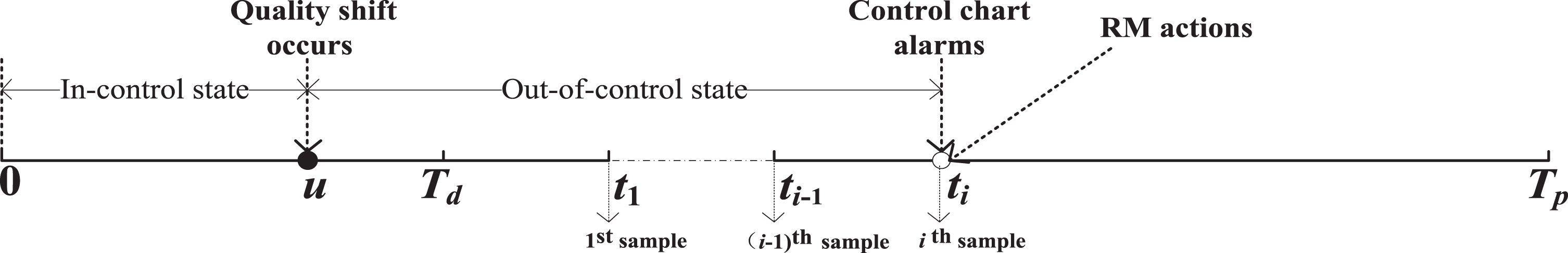
In S₁, a process quality shifts to out-of-control state at a time during the delayed monitoring period due to the occurrence of system deterioration, and control chart alarms at i^th sampling (i = 1, 2 ⋯ , L) which makes system stop at that time to perform RM. The operation process of the scenario can be illustrated in Fig. 2.

Fig. 2

An operation process of scenario 1 (S1).

A₁ represents the event that quality shift occurs in a very short period (u, u + du) during the delayed monitoring period (0, T_d); set B₁ as the event that the control chart alarms at the i^th sampling, and obviously the occurrence probability of the operation process is $\begin{matrix} P_{u (0, T_{d}), t_{i}} (S_{1}) = P (A_{1} \cap B_{1}) = P (A_{1}) P (B_{1} | A_{1}) \\ = f (u) du \cdot β^{i - 1} \cdot (1 - β) \end{matrix}$ (1)

As shown in Fig. 2, the system running time t_i = T_d + i · h, u is the length of in-control time, and t_i - u = T_d - u + i · h means the length of out-of-control time. In addition, the maintenance time is T₂. With consideration of system running time and the occurrence probability given above, the expected cycle time of the operation process is $\begin{matrix} {ET}_{u (0, T_{d}), t_{i}} (S_{1}) = \\ (T_{d} + i \cdot h + T_{2}) \cdot f (u) \cdot β^{i - 1} \cdot (1 - β) d u \end{matrix}$ (2)

Since RM is performed, maintenance cost is Cm₂. The quality loss is u · Cl₁ + (T_d - u + i · h) · Cl₂ which includes the loss of in-control process and out-of-control process. The sampling cost is i · Cs and shutdown loss is T₂ · Cd. Thus, we can obtain the expected cycle cost of the operation process as follows: $\begin{matrix} {EC}_{u (0, T_{d}), t_{i}} (S_{1}) = [{Cm}_{2} + u \cdot {Cl}_{1} \\ + (T_{d} - u + i \cdot h) \cdot {Cl}_{2} \\ + i \cdot Cs + T_{2} \cdot Cd] \cdot f (u) \cdot β^{i - 1} \cdot (1 - β) d u \end{matrix}$ (3)

Based on Equations (2) and (3), integrating u in the feasible domain (0, T_d), and considering all possible values of i (i = 1, 2,..., L), the expected cycle time and expected cycle cost of S₁ can be described as follows: $\begin{matrix} ET (S_{1}) \\ = \sum_{i = 1}^{L} \int_{0}^{T_{d}} (T_{d} + i \cdot h + T_{2}) \cdot f (u) \cdot β^{i - 1} \cdot (1 - β) d u \\ EC (S_{1}) \\ = \sum_{i = 1}^{L} \int_{0}^{T_{d}} [{Cm}_{2} + u \cdot {Cl}_{1} + (T_{d} - u + i \cdot h) \cdot {Cl}_{2} \end{matrix}$ (4) $\cdot f (u) \cdot β^{i - 1} \cdot (1 - β) d u$ (5)

3.2.2 Scenario 2 (S₂)

In S₂, a process quality shifts to out-of-control state at a time during the delayed monitoring period due to the occurrence of system deterioration, but no alert signal is given during all the control chart monitoring period, which makes the system run to the scheduled time of PM to perform RM. An operation process of the scenario can be illustrated in Fig. 3.

Fig. 3

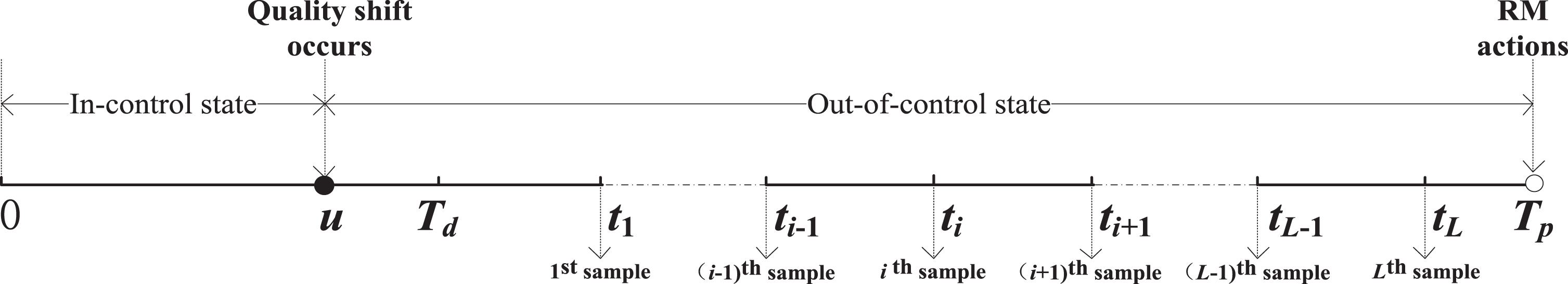
An operation Process of scenario 2 (S2).

Let A₂ be the event that the quality shift occurs in the very short period (u, u + du) during the delayed monitoring period (0, T_d), and B₂ be the event that the control chart does not alarm, the occurrence probability of the operation process can be expressed as follows: $\begin{matrix} P_{u (0, T_{d})} (S_{2}) = P (A_{2} \cap B_{2}) \\ = P (A_{2}) P (B_{2} | A_{2}) = f (u) d u \cdot β^{L} \end{matrix}$ (6)

From Fig. 3, it can be seen that the system running time is T_p, the length of in-control time is u, and the length of out-of-control time is T_p - u. RM is performed, so the maintenance time is T₂.

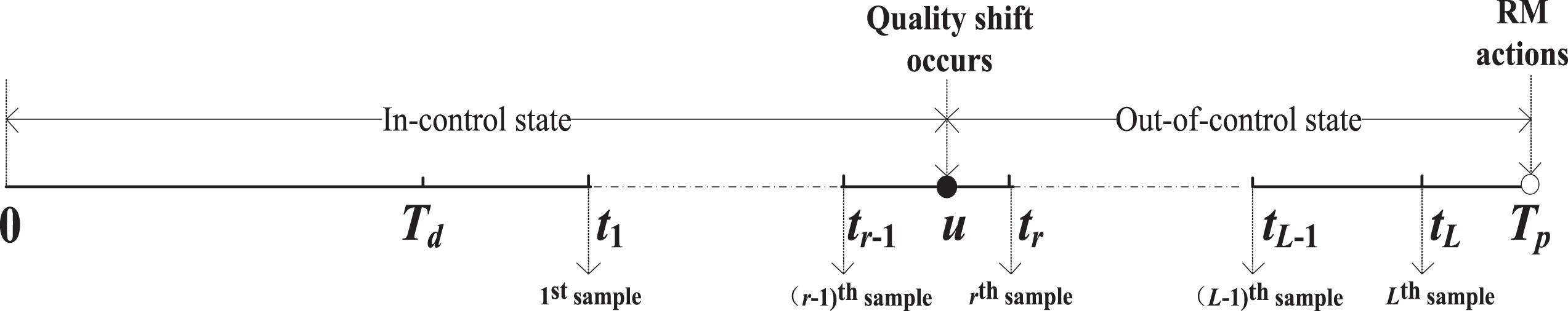
Based on Equation (6), integrating u in the feasible domain (0, T_d), then the expected cycle time and expected cycle cost of S₂ are $ET (S_{2}) = \int_{0}^{T_{d}} (T_{p} + T_{2}) \cdot f (u) \cdot β^{L} d u$ (7) $\begin{matrix} EC (S_{2}) = \int_{0}^{T_{d}} [{Cm}_{2} + u \cdot {Cl}_{1} + (T_{p} - u) \cdot {Cl}_{2} \\ + L \cdot Cs + T_{2} \cdot Cd] \cdot f (u) \cdot β^{L} du \end{matrix}$ (8)

3.2.3 Scenario 3 (S₃)

As shown in Fig. 4, a process quality shifts to out-of-control state between the (r-1)^th and r^th sampling due to the occurrence of system deterioration, and the control chart alarms at the j^th sampling (j = 1, 2 ⋯ , L) which makes the system stop at that time to perform RM. An operation process of the scenario can be illustrated in Fig. 4.

Fig. 4

An operation Process of scenario 3 (S3).

Suppose that A₃ is the event that quality shift occurs in the very short period (u, u + du) between the (r-1)^th and r^th sampling interval (r = 1, 2 ⋯ , L), and B₃ is the event that the control chart alarms at the j^th sampling (j = r, r + 1, ⋯ , L), then the occurrence probability of the operation process is $\begin{matrix} P_{u (t_{r - 1}, t_{r}), t_{j}} (S_{3}) = P (A_{3} \cap B_{3}) = P (A_{3}) P (B_{3} | A_{3}) \\ = f (u) d u \cdot (1 - a)^{r - 1} \cdot β^{j - r} \cdot (1 - β) \end{matrix}$ (9)

Based on Equation (9), integrating u in the feasible domain t_r-1, t_r (from Fig. 4, t_r-1 = (r - 1) · h + T_d, t_r = rh + T_d), and for all possible values of r (r = 1,2,...,L) and j (j = r,r + 1,..., L), the expected cycle time and expected cycle cost of S₃ are $\begin{matrix} ET (S_{3}) = \sum_{r = 1}^{L} \sum_{j = r}^{L} \int_{(r - 1) h + T_{d}}^{rh + T_{d}} (T_{d} + j \cdot h + T_{2}) \cdot f (u) \\ \cdot (1 - a)^{r - 1} \cdot β^{j - r} \cdot (1 - β) d u \end{matrix}$ (10) $\begin{matrix} EC (S_{3}) = \sum_{r = 1}^{L} \sum_{j = r}^{L} \int_{(r - 1) h + T_{d}}^{rh + T_{d}} \\ [{Cm}_{2} + u \cdot {Cl}_{1} + (T_{d} + j \cdot h - u) \cdot {Cl}_{2} \\ j \cdot Cs + T_{2} \cdot Cd] \cdot f (u) \cdot (1 - a)^{r - 1} \cdot β^{j - r} \cdot (1 - β) du \end{matrix}$ (11)

3.2.4 Scenario4 (S₄)

In S₄, a quality shift occurs during the monitoring period due to the system deterioration, but the control chart does not detect it during the subsequent sampling process, then the system keeps running until the scheduled time of PM to perform RM.

Because T_p - t_L < h (L is the maximum sampling number during scheduled duration of PM), according to the time and location of the quality shift, the analysis of this scenario must be further divided into the following two cases. In the first case, the shift occurs within any sampling interval before the L^th sampling during the monitoring period, which is called S₄₁; the second case S₄₂ is the situation that the shift occurs during the (t_L, T_p) period after the L^th sampling.

In S₄₁, process quality shift occurs between the (r-1)^th and r^th (r = 1,2,...,L) sampling during the monitoring period. An operation process of S₄₁ is illustrated in Fig. 5.

Fig. 5

An operation Process of scenario 4 (S41).

A₄₁ represents the event that quality shift occurs in the very short period (u, u + du) between the (r-1)^th and r^th sampling interval (r = 1, 2, ⋯ , L), and B₄₁ is the event that no alert signal is issued from the control chart. Then, the occurrence probability of the operation process can be obtained as follows: $\begin{matrix} P_{u (t_{r - 1}, t_{r})} (S_{41}) = P (A_{41} \cap B_{41}) \\ = P (A_{41}) P (B_{41} | A_{41}) \\ = f (u) d u \cdot (1 - a)^{r - 1} \cdot β^{L - r + 1} \end{matrix}$ (12)

From Fig. 5, the system running time is T_p, where u is the length of in-control time, and T_p - u is the length of out-of-control time. RM is performed and the value is T₂. Integrating u in the feasible domain (t_r-1, t_r), where t_r-1 = (r - 1) h + T_d, t_r = rh + T_d and taking into account different values of r (r = 1, 2,..., L), the expected cycle time and expected cycle cost of S₄₁ are $\begin{matrix} ET (S_{41}) = \sum_{r = 1}^{L} \int_{(r - 1) h + T_{d}}^{rh + T_{d}} (T_{p} + T_{2}) \\ \cdot f (u) \cdot (1 - a)^{r - 1} \cdot β^{L - r + 1} du \end{matrix}$ (13) $\begin{matrix} EC (S_{41}) = \sum_{r = 1}^{L} \int_{(r - 1) h + T_{d}}^{rh + T_{d}} \\ [{Cm}_{2} + u \cdot {Cl}_{1} + (T_{p} - u) \cdot {Cl}_{2} \\ + L \cdot Cs + T_{2} \cdot Cd] \cdot f (u) \cdot (1 - a)^{r - 1} \cdot β^{L - r + 1} du \end{matrix}$ (14)

In S₄₂, process quality shift occurs after the L^th sampling, which is shown in Fig. 6. Since L is the maximum number of sampling during the scheduled duration of PM, T_p - T_L ⩽ h, and t_L ⩽ u ⩽ T_p.

Fig. 6

An Operation Process of scenario 4 (S42).

Let A₄₂ be the event that quality shift occurs in a very short period (u, u + du) during the period of (t_L, T_p), and B₄₂ be the event that the control chart does not alarm all the time. Then the occurrence probability of the operation process is $\begin{matrix} P_{u (t_{L}, T_{p})} (S_{42}) = P (A_{42} \cap B_{42}) = \\ P (A_{42}) P (B_{42} | A_{42}) = f (u) d u \cdot (1 - a)^{L} \end{matrix}$ (15)

Integrating u in the feasible domain (t_L, T_p), where t_L = L · h + T_d, then the expected cycle time and expected cycle cost of S₄₂ are $ET (S_{42}) = \int_{Lh + T_{d}}^{T_{p}} (T_{p} + T_{2}) \cdot f (u) \cdot (1 - a)^{L} d u$ (16) $\begin{matrix} EC (S_{42}) = \int_{Lh + T_{d}}^{T_{p}} [{Cm}_{2} + u \cdot {Cl}_{1} + (T_{p} - u) \cdot {Cl}_{2} \\ + L \cdot Cs + T_{2} \cdot Cd] \cdot f (u) \cdot (1 - a)^{L} du \end{matrix}$ (17)

Combine the two cases above, the expected cycle time and expected cycle cost of S₄ are $ET (S_{4}) = ET (S_{41}) + ET (S_{42})$ (18) $EC (S_{4}) = EC (S_{41}) + EC (S_{42})$ (19)

3.2.5 Scenario 5 (S₅)

As to S₅, no deterioration and no quality shift occur during the whole operation process, but the control chart alarms (it is a false alert signal), resulting in CM at the alarm point. Suppose that the control chart issues a false alert signal (type I error) at the i^th (i = 1, 2, ⋯ , L) sampling, then an operation process of S₅ can be shown in Fig. 7.

Fig. 7

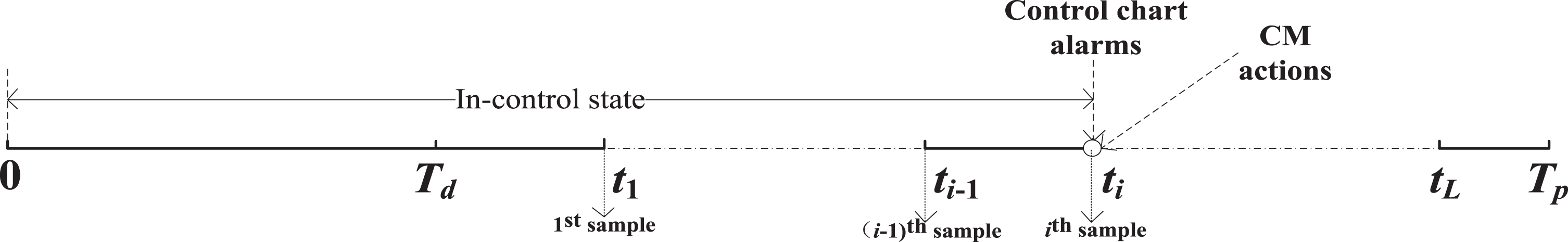
An operation process of scenario 5 (S5).

Define A₅ as the event that the system is always good within t_i, and B₅ as the event that the control chart alarms at the i^th sampling. Then, the occurrence probability of the operation process is $\begin{matrix} P_{t_{i}} (S_{5}) = P (A_{5} \cap B_{5}) = P (A_{5}) P (B_{5} | A_{5}) \\ = [1 - F (t_{i})] \cdot (1 - a)^{i - 1} a \end{matrix}$ (20)

From Fig. 7, t_i = T_d + ih is the system running time, where t_i = T_d + ih is the length of in-control time, and the length of out-of-control time is 0. Since the alert signal is false, at this time the system operates in control and there is no need to replace or repair the parts but lubricate. Namely, CM is performed. For all possible values of i (i = 1, 2,..., L), the expected cycle time and expected cycle cost of S₅ are $\begin{matrix} ET (S_{5}) = \\ \sum_{i = 1}^{L} (T_{d} + i \cdot h + T_{1}) \cdot [1 - F (t_{i})] \cdot (1 - a)^{i - 1} \cdot a \end{matrix}$ (21) $\begin{matrix} EC (S_{5}) = \sum_{i = 1}^{L} [{Cm}_{1} + (T_{d} + i \cdot h) \cdot {Cl}_{1} + i \cdot Cs \\ + T_{1} \cdot Cd] \cdot [1 - F (t_{i})] \cdot (1 - a)^{i - 1} \cdot a \end{matrix}$ (22)

3.2.6 Scenario 6 (S₆)

In S₆, neither system deterioration nor alter signal occurs, so the system remains running till the scheduled time of PM to perform PM. The operation process of S₆ is shown in Fig. 8.

Fig. 8

Operation Process of scenario 6 (S6).

Define A₆ as the event that the system is always good within T_p, and B₆ as the event that the control chart does not alarm all the time. The probability that the process keeps in-control state during the entire operation process is the reliability of the system and equals to P_{T
_p} (S₆) = P (A₆ ∩ B₆) = P (A₆) P (B₆|A₆); the probability that control chart does not issue false signal from the first to L^th sampling is [1 - F (T_p)] · (1 - a) ^L. So, the occurrence probability of S₆ is $\begin{matrix} P_{T_{p}} (S_{6}) = P (A_{6} \cap B_{6}) = P (A_{6}) P (B_{6} | A_{6}) \\ = [1 - F (T_{p})] \cdot (1 - a)^{L} \end{matrix}$ (23)

It can be seen from Fig. 8 that the system running time is T_p, where the length of in-control time is T_p and the length of out-of-control time is 0. Although the system still operates in-control, PM must be performed to reduce the risk of system deterioration. As a result, the expected cycle time and expected cycle cost of S₆ are $ET (S_{6}) = (T_{p} + T_{3}) \cdot [1 - F (T_{p})] \cdot (1 - a)^{L}$ (24) $\begin{matrix} EC (S_{6}) = ({Cm}_{3} + T_{p} \cdot {Cl}_{1} + L \cdot Cs + T_{3} \cdot Cd) \\ \cdot [1 - F (T_{p})] \cdot (1 - a)^{L} \end{matrix}$ (25)

3.3 Optimization model

By considering the above-mentioned scenarios, the expected system cost function per unit time can be obtained in Equation (26) by the renewal theory. Hence, the objective of the joint economic design of PM and $\bar{X}$ chart based on delayed monitoring is to minimize ECT by optimizing the values of scheduled duration of PM (T_p), delayed monitoring duration (T_d) and $\bar{X}$ chart parameters (n,h,k).

$\begin{matrix} ECT = \\ \frac{EC (S_{1}) + EC (S_{2}) + EC (S_{3}) + EC (S_{4}) + EC (S_{5}) + EC (S_{6})}{ET (S_{1}) + ET (S_{2}) + ET (S_{3}) + ET (S_{4}) + ET (S_{5}) + ET (S_{6})} \end{matrix}$ (26)

4 Numerical investigation and solution procedure

Numerical simulation is carried out to illustrate the resolution approach and to compare the model presented. And Imperialist Competitive Algorithm (ICA) is employed to optimize the decision variables T_p, T_d, n, h, k in order to obtain the minimal value of ECT. Also the sensitivity analysis of the model is explored.

4.1 Solution procedure

ICA is a stochastic optimization algorithm to simulate human social colonial competition [30]. It has been successfully applied to supply chain optimization [31, 32], production scheduling [33 –35], information classification [36] and multi-objective optimization [37] and has been proved to have a better effect on the continuous optimization problem with less iteration [37]. The specific algorithm processes of the model in this paper are described as follows:

Step 1. Generate an initial empire. Randomly generate 100 countries, calculate the ECT of each country according to Equation (26), and select the top 5 countries as the initial empire according to the order of ECT from small to large. At the same time, allocate the number of colonies based on their powers.

Step 2. Colonial Assimilation. Colonial assimilation is a process that a colonial nation gradually moves toward its empires. It is represented in the algorithm as a process in which the colonial countries approach its empires continuously (assimilation coefficient θ= 2, deviation angle γ = π/4); in this process, if the colonial ECT is better than that of the empires, then the colony replaces imperialist and the colonies approach the new empires.

Step 3. Empire competition. Calculate the total strength of each empire (weighting factor ɛ = 0.1) according to the weighted sum of the target values of the colonial countries and the empires, and rank the empires according to the size of power. Then assign the weakest colony of the weakest empire to the most probable empire. If there is only one colony left in the weakest empire, this empire will die.

Step 4. Evaluate the number of empires.

Step 5. Loop operation and output. If there is just one empire, stop. If not, go to step 2 until there is only one empire remaining. Then end the algorithm and output the result.

4.2 A numerical example

Consider a casting production process in a mold manufacturing company to illustrate the effectiveness of the joint model. The quality characteristic of castings X approximately has a normal distribution. When the production system is in in-control state, X∼N (3.2, 1), and the process quality shifts to μ =μ₀ +δ₁ σ₀ = 4.2 when the system shifts to out-of-control state. According to the historical data, the occurrence time of quality shift caused by the system deterioration has a Weibull distribution with shape parameter Beta = 1.8 and scale parameter Theta = 1000 hours. Other relevant time and cost parameter values are listed in Table 2.

Table 2
Time and cost parameter values of a casting process

Time/Cost parameter T ₁ T ₂ T ₃ Cm ₁ Cm ₂ Cm ₃ Cl ₁ Cl ₂ Cd C_f C_q

Value 1 6 4 126 5000 2000 2 86 360 216 2

Time/Cost parameter	T ₁	T ₂	T ₃	Cm ₁	Cm ₂	Cm ₃	Cl ₁	Cl ₂	Cd	C_f	C_q
Value	1	6	4	126	5000	2000	2	86	360	216	2

Note: The unit of time parameter is hour and that of cost parameter is Yuan.

Based on data from the case, the ICA is employed to solve our model with MATLAB (R2014a) software. Table 3 shows the optimal results. The values of the optimal variables that minimize ECT are T_p = 1545.7875, T_d = 238.0952, n = 7, h = 18.3385, k = 2.7154, and the corresponding hourly cost is ECT = 20.8065.

Table 3

Results of the proposed model

Parameter	ECT	T_p	T_d	n	h	k
Optimal value	20.8065	1545.7875	238.0952	7	18.3385	2.7154

4.3 Comparison analysis

To further verify the economic superiority of our model (M₁), the economic performance of our model is demonstrated by comparing with the model without delayed monitoring policy (M₂) when taking into account different values of quality shift distribution parameters. Let T_d = 0, we can conveniently obtain the integrated model without delayed monitoring policy. Based on the time and cost parameters in Table 2, we can calculate different ECT values of M₁ and M₂ when Beta and Theta take different values and Table 4 reports the results.

Table 4
ECT comparison for the proposed model and the comparison model

Beta Theta = 1000 Theta = 1500 Theta = 2000

M ₁ M ₂ M₂-M₁ M ₁ M ₂ M₂-M₁ M ₁ M ₂ M₂-M₁

1.0 24.1014 23.4265 –0.6749 21.5679 21.5069 –0.0610 17.8758 18.6627 0.7869

1.5 22.5565 23.2772 0.7207 19.4226 20.7848 1.3622 16.8930 18.3240 1.4310

2.0 20.9338 22.7660 1.8322 17.7094 20.0141 2.3047 13.1928 17.6591 4.4663

2.5 17.8460 21.1301 3.2841 13.4687 19.0569 5.5882 10.8503 17.2811 6.4308

Beta	Theta = 1000	Theta = 1500	Theta = 2000
1.0	24.1014	23.4265	–0.6749	21.5679	21.5069	–0.0610	17.8758	18.6627	0.7869
1.5	22.5565	23.2772	0.7207	19.4226	20.7848	1.3622	16.8930	18.3240	1.4310
2.0	20.9338	22.7660	1.8322	17.7094	20.0141	2.3047	13.1928	17.6591	4.4663
2.5	17.8460	21.1301	3.2841	13.4687	19.0569	5.5882	10.8503	17.2811	6.4308

Table 4 shows (M₂-M₁) is positively correlated with the Beta value and Theta value, that is, the delayed monitoring effect strengthens with the increasing of Beta and Theta. This is because in the early operation of the system, the equipment failure rate will decrease with the increasing of Beta and Theta. The lower the probability of failure is, the less necessary and effective for the control chart to monitor the state of the equipment, then, the more effective of delayed monitoring.

4.4 Sensitivity analysis

In order to provide decision-making reference for process management optimization, we use the orthogonal experimental design and regression analysis method to analyze the different effect of model parameters on ECT.

4.4.1 Parameters and experiment design

Table 5 presents the two levels of twelve model parameters (δ₁, T₁, T₂, T₃, Cl₁, Cl₂, Cm₁, Cm₂, Cm₃, Cd, Cf, Cq). L₁₆ (2¹²) is chosen for orthogonal experiment design and Table 6 presents the sixteen test schedules. The results of the sixteen tests are shown in Table 7 by using ICA with MATLAB (R2014a) software.

Table 5
Parameter- level setting in the proposed model

Parameter δ ₁ T ₁ T ₂ T ₃ Cl ₁ Cl ₂ Cm ₁ Cm ₂ Cm ₃ Cd Cf Cq

Level1 0.5 1 4.5 2.5 5 50 10 400 100 400 50 2

Level2 1 2 9 5 10 100 20 800 200 800 100 4

Parameter	δ ₁	T ₁	T ₂	T ₃	Cl ₁	Cl ₂	Cm ₁	Cm ₂	Cm ₃	Cd	Cf	Cq
Level1	0.5	1	4.5	2.5	5	50	10	400	100	400	50	2
Level2	1	2	9	5	10	100	20	800	200	800	100	4

Table 6

Orthogonal Experiment Design

No.	δ ₁	T ₁	T ₂	T ₃	Cl ₁	Cl ₂	Cd	Cf	Cm ₁	Cm ₂	Cm ₃	Cq
1	1	1	1	1	1	1	1	1	1	1	1	1
2	1	1	1	1	1	1	1	2	2	2	2	2
3	1	1	1	2	2	2	2	1	1	1	1	2
4	1	1	1	2	2	2	2	2	2	2	2	1
5	1	2	2	1	1	2	2	1	1	2	2	1
6	1	2	2	1	1	2	2	2	2	1	1	2
7	1	2	2	2	2	1	1	1	1	2	2	2
8	1	2	2	2	2	1	1	2	2	1	1	1
9	2	1	2	1	2	1	2	1	2	1	2	1
10	2	1	2	1	2	1	2	2	1	2	1	2
11	2	1	2	2	1	2	1	1	2	1	2	2
12	2	1	2	2	1	2	1	2	1	2	1	1
13	2	2	1	1	2	2	1	1	2	2	1	1
14	2	2	1	1	2	2	1	2	1	1	2	2
15	2	2	1	2	1	1	2	1	2	2	1	2
16	2	2	1	2	1	1	2	2	1	1	2	1

Table 7

ECT value for the numerical example

No.	ECT	No.	ECT	No.	ECT	No.	ECT
1	12.2524	5	30.6891	9	20.8317	13	21.5637
2	22.5480	6	25.3722	10	24.7843	14	22.9191
3	34.1354	7	28.2467	11	17.2152	15	15.8533
4	38.7691	8	24.4023	12	20.1216	16	13.8974

4.4.2 Regression analysis

Based on the above test results, we run the regression analysis (a = 0.05) to the response variable ECT by using Minitab software. Table 8 presents the variance analysis and the main regression effect and Table 9 reports the results of regression coefficient significance test.

Table 8
Regression variance analysis and general effect of ECT

Source D.f. SS MS F-ratio P-value S R-Sq R-Sq (adjustment)

Regression 12 759.291 63.274 27.10 0.01 1.52813 99.1% 95.4%

Residual error 3 7.006 2.335

Total 15 766.296

Source	D.f.	SS	MS	F-ratio	P-value	S	R-Sq	R-Sq (adjustment)
Regression	12	759.291	63.274	27.10	0.01	1.52813	99.1%	95.4%
Residual error	3	7.006	2.335
Total	15	766.296

Table 9

Significance tests on regression coefficient of ECT

Independent variable	Coefficient	Standard error	T-ratio	P-value
constant	–7.299	3.989	–1.83	0.165
δ ₁	–14.807	1.528	–9.69	0.002
T ₁	–0.9642	0.7641	–1.26	0.296
T ₂	0.2701	0.1698	1.59	0.210
T ₃	0.5840	0.3056	1.91	0.152
Cl ₁	1.4426	0.1528	9.44	0.003
Cl ₂	0.11992	0.01528	7.85	0.004
Cd	0.43829	0.07641	5.74	0.011
Cf	0.003758	0.001910	1.97	0.144
Cm ₁	–0.000613	0.007641	–0.08	0.941
Cm ₂	0.009859	0.001910	5.16	0.014
Cm ₃	0.04158	0.01528	2.72	0.072
Cq	0.5342	0.3820	1.40	0.256

As can be seen in Table 8, the P-value = 0.01 < 0.05, indicating that there is a significant correlation between response variables and predictive variables, that is, at least one parameter significantly affect the ECT; also, R-sq and R-sq (adjustment) are very close, showing that the regression model is reliable; R-sq (adjustment) = 95.4%, implying that the fitting model can explain 95.4%variation in ECT, and the regression model agrees very well with the data. Moreover, from Table 9, it can be seen that the factors with P-value < 0.05 are δ₁, Cl₁, Cl₂, Cd and Cm₂, indicating that these five factors have significant influences on the ECT change. From the main effect analysis results (Fig. 9), ECT decreases with the increasing of δ₁, and increases with the increasing of Cl₁, Cl₂, Cd and Cm₂. It suggests that δ₁ shows negative effects on ECT, while Cl₁, Cl₂, Cd and Cm₂ show positive effects.

Fig. 9

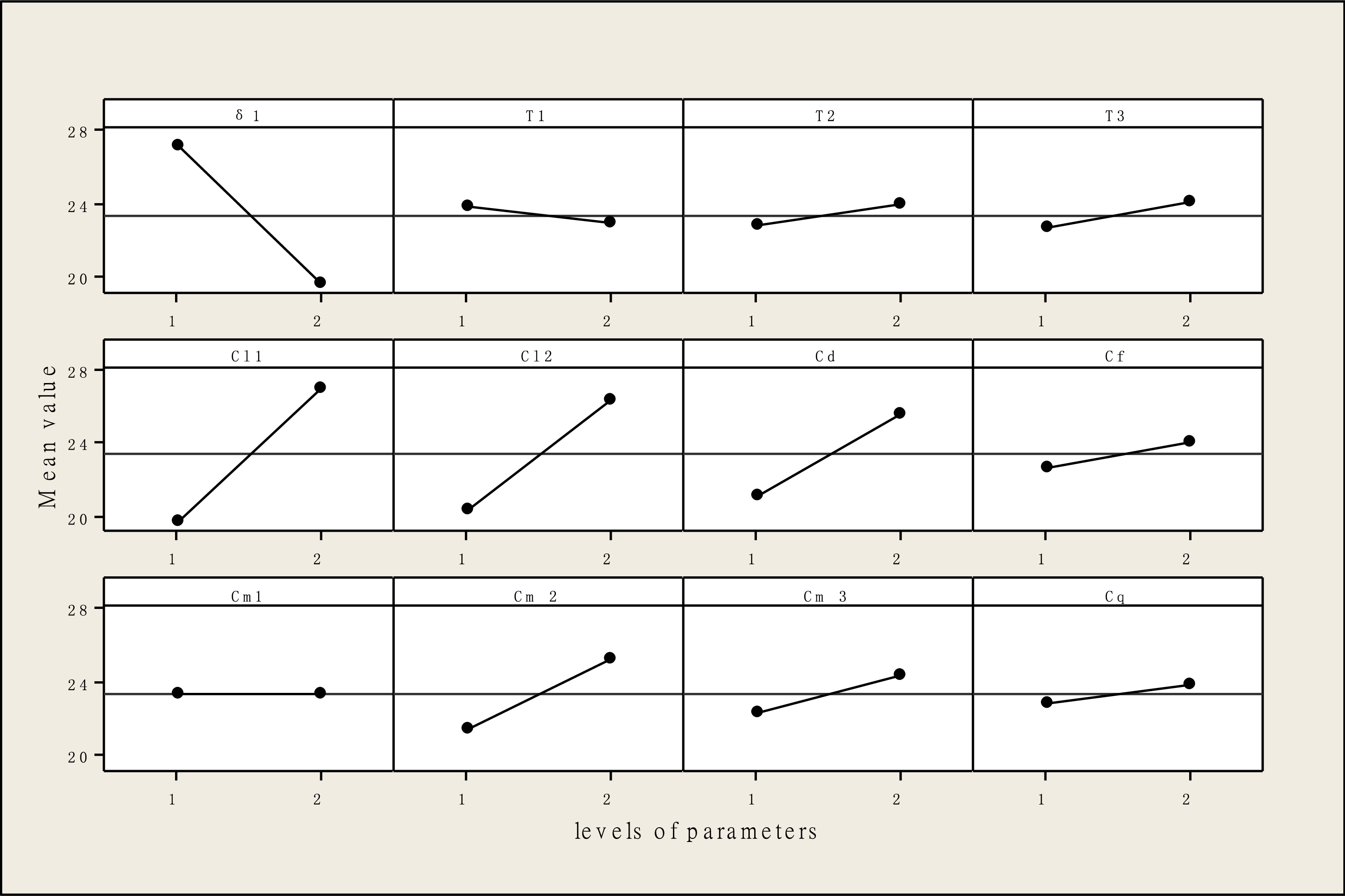
Main effects plot.

4.4.3 Analysis of results and discussion

Among the five factors that significantly affect ECT, Cl₁, Cl₂, Cd and Cm₂ have positive influences because they are used as cost parameters, and with the increasing of their values, the renewal cost of the system will increase, which results in the increasing of ECT. δ₁ shows negative effects because the larger of δ₁ is, the greater of the process shifts, then it is easier for the control chart to detect the out-of-control state. The shorter the out-of-control time is, the less the out-of-control cost is, and the smaller the ECT is.

As for Cm₁ and Cm_3, they have no-significant influences on ECT, which may be related to the relatively small occurrence probabilities of CM and PM. For CM, RM and PM, both true alert signal and false alert signal made by the control chart result in RM; during the operation, due to the monitoring effect of the control chart, the shutdown maintenance is mainly resulted by the true alert signal, so RM has the highest probability in the three kinds of maintenance. In this paper, ECT represents the expected cost per unit time of each of these scenarios, and the greater the occurrence probability of the scenario, the more significant the impact of maintenance costs on ECT. Consequently, Cm₂ has a significant effect on ECT while Cm₁ and Cm₃ are not significant.

5 Conclusion

This study considers a joint decision model for PM and control chart from the point of cost. Due to taking delayed monitoring into account, it can achieve a superior economic performance to the model without delayed monitoring period for the system with a low hazard rate during the early age of the production process.

According to the sensitivity analysis, it can be observed that Cl₁, Cl₂, Cd and Cm₂ demonstrate a significantly positive effect on ECT, thereby improving the management level of production operations to reduce the quality loss per unit time. Also, the management performance of RM should be improved to reduce the corresponding operation cost; furthermore, unplanned shutdown maintenance should be minimized as much as possible or maintenance and repair work should be arranged in the production interval to reduce the production shutdown and the cost per unit time for the renewal cycle.

The control chart involved in this model is a fixed parameters control chart. And there are usually multiple quality characters shifts when an equipment deterioration or failure occurs in practice. More than this, the quality characters could be relevant or auto-correlated. Therefore, further researcher efforts can be made in integrating other control charts, e.g., dynamic control chart, control chart for monitoring multivariate auto-correlated processes and else. In addition, on account of the high computational complexity of the integrated model, other potential optimization algorithms can also be adapted as a solution procedure.

Footnotes

Acknowledgments

The authors gratefully acknowledge the financial supports from the Nation Natural Science of China (No. U1404702 and 71871204), Program for Innovative Research Team (in Science and Technology) in University of Henan Province (No. 21RTSTHN018), the Humanities and Social Sciences Foundation of Ministry of Education of China (No.20YJCZH235), Science and Technology Project of Henan Science and Technology Department, China (No. 212102210338).

References

Savino

M.M.

, Brun

and Riccio

, Integrated system for maintenance and safety management through FMECA principles and fuzzy inference engine, European Journal of Industrial Engineering 5(2) (2011), 132–169.

Bahria

, Chelbi

, Dridi

I.H.

and Bouchriha

, Maintenance and quality control integrated strategy for manufacturing systems, European J. Industrial Engineering 12(3) (2018), 307–331.

Park

, Optimal production policy for economic production lot-sizing model with preventive maintenance[J], Quality Technology and Quantitative Management 2020(2), 1–18.

Liao

, Chen

and Yang

, Joint optimization of preventive maintenance and production scheduling for parallel machines system[J], Journal of Intelligent & Fuzzy Systems 32(1) (2017).

Bouslah

, Gharbi

and Pellerin

, Integrated production, sampling quality control and maintenance of deteriorating production systems with AOQL constraint, Omega 61(4) (2016), 110–126.

Lesage

and Dehombreux

, Simulation of manufacturing processes subject to maintenance and quality control: sensitivity analysis and numerical example, International Journal of Mechanical Engineering and Automation 2(3) (2015), 119–126.

Pandey

, Kulkarni

M.S.

and Vrat

, Joint consideration of production scheduling, maintenance and quality policies: a review and conceptual framework, International Journal of Advanced Operations Management 2(1) (2010), 1–24.

Linderman

, Mckone-sweet

K.E.

and Anderson

J.C.

, An integrated systems approach to process control and maintenance, European Journal of Operational Research 164(2) (2005), 324–340.

Zhou

and Zhu

, Economic design of integrated model of control chart and maintenance management, Mathematical & Computer Modelling 47(11) (2008), 1389–1395.

10.

Mehrafrooz

and Noorossana

, An integrated model based on statistical process control and maintenance, Computers & Industrial Engineering 61(4) (2011), 1245–1255.

11.

Yin

, Zhang

, Zhu

, et al., An integrated model of statistical process control and maintenance based on the delayed monitoring, Reliability Engineering and System Safety 133 (2015), 323–333.

12.

Xiang

, Joint optimization of

\bar{X}

control chart and preventive maintenance policies: A discrete-time Markov chain approach, European Journal of Operational Research 229(2) (2013), 382–390.

13.

Liu

, Jiang

and Zhang

, An integrated model of statistical process controland condition-based maintenance for deteriorating systems, Journal of the Operational Research Society 68(11) (2017), 1452–1460.

14.

Panagiotidou

and Nenes

, An economically designed, integrated quality and maintenance model using an adaptive Shewhart chart, Reliability Engineering & System Safety 94(3) (2009), 732–741.

15.

Liu

, Yu

, Ma

, et al., Economic and economic-statistical designs of an

\bar{X}

control chart for two-unit series systems with condition-based maintenance, European Journal of Operation Research 226(3) (2013), 491–499.

16.

Zhong

and Ma

, An integrated model based on statistical process control and maintenance for two-stage dependent processes, Communications in Statistics-Simulation and Computation 46(1) (2014), 106–126.

17.

Rasay

, Fallahnezhad

M.S.

and Zaremehrjerdi

, An integrated model of statistical process control and maintenance planning for a two-stage dependent process under general deterioration, European Journal of Industrial Engineering 13(2) (2019), 149–177.

18.

Mehdi

, Nidhal

and Anis

, Integrated maintenance and control policy based on quality control, Computers & Industrial Engineering 58(3) (2010), 443–451.

19.

Yin

and Makis

, Economic and economic-statistical design of a multivariate Bayesian control chart for condition-based maintenance, IMA Journal of Management Mathematics 22(1), 47–63.

20.

Wang

, A simulation-based multivariate Bayesian control chart for real time condition-based maintenance of complex systems, European Journal of Operational Research 218(3) (2012), 726–734.

21.

Salmasnia

, Kaveie

and Namdar

, An integrated production and maintenance planning model underVP-T² Hotelling chart, Computers & Industrial Engineering 118(4) (2018), 89–103.

22.

, Chen

and Pan

, Joint economic design of CUSUM control chart and age-based imperfect preventive maintenance policy, Mathematical Problems in Engineering 2018(6) (2018), 1–11.

23.

Khrueasom

and Pongpullponsak

, The integrated model of the Kolmogorov–Smirnov distribution-freestatistic approach to process control and maintenance,–, Science 29(2) (2017), 182–190.

24.

Charongrattanasakul

and Pongpullponsak

, Minimizing the cost of integrated systems approach to process control and maintenance model by EWMA control chart using genetic algorithm, Expert Systems with Applications An International Journal 38(5) (2011), 5178–5186.

25.

, Liu

, Cui

, et al., Reliability-oriented design of integrated model of preventive maintenance and quality control policy with time-between-events control chart, Computers & Industrial Engineering 129 (2019), 228–238.

26.

Bouslah

, Gharbi

and Pellerin

, Joint production, quality and maintenance control of a two-machine line subject to operation- dependent and quality-dependent failures, International Journal of Production Economics 195 (2018), 210–226.

27.

Cheng

, Zhou

and Li

, Integrated production, quality control and condition-based maintenance for imperfect production systems, Reliability Engineering & System Safety 175 (2018), 251–264.

28.

Salmasnia

, Soltani

, Heydari

, et al., An integrated model for joint determination of production run length, adaptive control chart parameters and maintenance policy, Journal of Industrial and Production Engineering 36(6) (2019), 401–417.

29.

Cheng

C.Y.

, Zhao

X.F.

, Chen

, et al., A Failure-rate-reduction Periodic Preventive Maintenance Model with Delayed Initial Time in a Finite Time Period[J], Quality Technology & Quantitative Management 11(3) (2014), 245–254.

30.

Atashpaz-Gargari

and Lucas

, Imperialist competitive algorithm: An algorithm for optimization inspired byimperialistic competition. Evolutionary Computation, CEC 2007. IEEE Congress on. IEEE 2007 (2007), 4661–4667.

31.

Ahmadzadeh

and Vahdani

, A location-inventory-pricing model in a closed loop supply chain network with correlated demands and shortages under a periodic review system, Computers & Chemical Engineering 101(6) (2017), 148–166.

32.

Kermani

M.A.M.A.

, Aliahmadi

, Salamat

V.R.

, et al., Supplier selection in a single-echelon supplychain with horizontal competition using Imperialist competitive algorithm, International Journal of Computer Integrated Manufacturing 28(6) (2015), 628–638.

33.

Ramezanian

, Mohammadi

and Cheraghalikhani

, Toward an integrated modeling approach for production and delivery operations in flow shop system: Trade-off between direct and routing delivery methods, Journal of Manufacturing Systems 44(7) (2017), 79–92.

34.

Seidgar

, Zandieh

and Mahdavi

, Bi-objective optimization for integrating production and preventive maintenance scheduling in two-stage assembly flow shop problem, Journal of the Chinese Institute of Industrial Engineers 33(6) (2016), 404–425.

35.

Ghorbani

, Esmaeili

and Alizadeh

, Improving OPTICS algorithm with imperialist competitive algorithm: choosing automatically best parameters, Advances in Computer Science: an International Journal 5(3) (2016), 21–27.

36.

Bilel

, Mohamed

N.Z.

, et al., An improved imperialist competitive algorithm for multi-objective optimization, Engineering Optimization 48(11) (2016), 1823–1844.

37.

Nikmehr

and Ravadanegh

S.N.

, Imperialist competitive algorithm: an algorithm for optimization inspired by imperialistic competition, Journal of Renewable & Sustainable Energy 21(1) (2015), 4661–4667.

Joint decision-making model of preventive maintenance and delayed monitoring SPC based on imperialist competitive algorithm

Abstract

Keywords

1 Introduction

2 Assumptions and notations

3.1 System analysis

3.2.1 Scenario 1 (S1)

4.1 Solution procedure

4.2 A numerical example

Table 2 Time and cost parameter values of a casting process Time/Cost parameter T 1 T 2 T 3 Cm 1 Cm 2 Cm 3 Cl 1 Cl 2 Cd C f C q Value 1 6 4 126 5000 2000 2 86 360 216 2

4.4.1 Parameters and experiment design

Table 5 Parameter- level setting in the proposed model Parameter δ 1 T 1 T 2 T 3 Cl 1 Cl 2 Cm 1 Cm 2 Cm 3 Cd Cf Cq Level1 0.5 1 4.5 2.5 5 50 10 400 100 400 50 2 Level2 1 2 9 5 10 100 20 800 200 800 100 4

Table 8 Regression variance analysis and general effect of ECT Source D.f. SS MS F-ratio P-value S R-Sq R-Sq (adjustment) Regression 12 759.291 63.274 27.10 0.01 1.52813 99.1% 95.4% Residual error 3 7.006 2.335 Total 15 766.296

5 Conclusion

Footnotes

Acknowledgments

References

3.2.1 Scenario 1 (S₁)

Table 2
Time and cost parameter values of a casting process

Time/Cost parameter T ₁ T ₂ T ₃ Cm ₁ Cm ₂ Cm ₃ Cl ₁ Cl ₂ Cd C_f C_q

Value 1 6 4 126 5000 2000 2 86 360 216 2

Table 5
Parameter- level setting in the proposed model

Parameter δ ₁ T ₁ T ₂ T ₃ Cl ₁ Cl ₂ Cm ₁ Cm ₂ Cm ₃ Cd Cf Cq

Level1 0.5 1 4.5 2.5 5 50 10 400 100 400 50 2

Level2 1 2 9 5 10 100 20 800 200 800 100 4

Table 8
Regression variance analysis and general effect of ECT

Source D.f. SS MS F-ratio P-value S R-Sq R-Sq (adjustment)

Regression 12 759.291 63.274 27.10 0.01 1.52813 99.1% 95.4%

Residual error 3 7.006 2.335

Total 15 766.296