An automatic brain tumor segmentation using modified inception module based U-Net model

Abstract

Manual segmentation of brain tumor is not only a tedious task that may bring human mistakes. An automatic segmentation gives results faster, and it extends the survival rate with an earlier treatment plan. So, an automatic brain tumor segmentation model, modified inception module based U-Net (IMU-Net) proposed. It takes Magnetic resonance (MR) images from the BRATS 2017 training dataset with four modalities (FLAIR, T1, T1ce, and T2). The concatenation of two series 3×3 kernels, one 5×5, and one 1×1 convolution kernels are utilized to extract the whole tumor (WT), core tumor (CT), and enhance tumor (ET). The modified inception module (IM) collects all the relevant features and provides better segmentation results. The proposed deep learning model contains 40 convolution layers and utilizes intensity normalization and data augmentation operation for further improvement. It achieved the mean dice similarity coefficient (DSC) of 0.90, 0.77, 0.74, and the mean Intersection over Union (IOU) of 0.79, 0.70, 0.70 for WT, CT, and ET during the evaluation.

Keywords

Brain tumor automatic segmentation deep neural network inception convolution

1 Introduction

A brain tumor is one of the deadliest tumors among people. There are several types of brain tumors available, where glioma is one of the primary tumors. It originates from the Glial cells [5]. Medical clinics diagnose a brain tumor with several methods in which analysis with images like Computed Tomography, Magnetic resonance imaging (MRI) are the most used method by a medical practitioner. MRI is preferable [9] because it gives a better image of soft tissues, organs, and it has a good signal-to-noise ratio compared to other imaging examinations. The World Health Organization (WHO) classifies glioma into four categories from grade I to IV [14 , 37] depends on malignancy level. WHO again classified glioma into two categories as Low-Grade Glioma (LGG) and High-Grade Glioma (HGG) based on the growth of cancer cells and the seriousness of glioma [5, 23]. LGG consists of grades II and III. HGG consists of grade IV. Manual segmentation of glioma is a complex task that takes more time to detect, localize, classify and segment tumors. The semi or fully automatic segmentation model has a deep neural network (DNN) which segments tumors and provides better results than manual segmentation. DNN plays a vital role in the healthcare field like disease detection, disease classification, decision making [29], tumor segmentation, etc. The medical practitioner gives immediate medication, therapy, surgery with these technology improvements. A dual pathway 3D CNN [19] with the 3D fully connected conditional random field (CRF) has 11 deep layers to detect brain lesions. A DNN [33] model detects plant disease, which gets leaf images and categorizes 13 diseases with an average precision of 94%. A Multi-scale Dense U-Net (MDU-Net) method [42] segments biomedical images. It minimizes overfitting issues and gives better accuracy. A DNN model with scaled principal component analysis (PCA) [22] is used to detect osteoarthritis earlier. It has been achieved by using statistical data which were collected from hospitals. A MultiResUNet [17] method has to segment multimodal biomedical images [10] that give better results compared to the original U-Net architecture [30].

2 Related work

Many researchers are working towards a fully automatic segmentation of brain tumors. Few research works are discussed in this section. A modified version [34] of the U-Net [30] and VGG16 architecture [31] method consists of two models to segment various brain tumor regions. The first model has 23-layers to segment WT from T2, FLAIR MRI modalities, and another model has 18-layers to segment enhance tumor (ET) and core tumor (CT) from T1ce MRI modality of a subject. The deep network has two modules; feature reuse and feature conformity modules [18]. The first module extracts more relevant features at each level, and another module removes noise and then enhances the fusion of feature maps. The feature reuse module is a modified version of the residual block with an additional 1×1 convolution layer in the residual path. The feature conformity module carries two parallel convolution layers with skip connections to limit noise from the direct fusion process. A triple cascade CNN [41] model has three CNN networks; WNet, TNet, and ENet are used to segment WT, CT, and ET subsequently. Bounding box automatically created in a training phase based on the labeled data available in the dataset and bounding box generated based on the segmentation results during the testing phase. It has multiple layers of the residual block with dilated convolution filters and anisotropic filters to improve segmentation performance.

A fully connected CNN SegNet [1] model segments WT and tumor parts such as edema, necrosis, ET. The evaluation of the model has been done by using BRATS 2017 datasets [3, 4]. The training parameters in the encoder block are less compared to VGG16 architecture. The CNN model with a 3×3 kernel [25] has two different architectures for HGG and LGG. An HGG model consists of 11 layers of CNN architecture, and an LGG model consists of 9 layers of CNN architecture. It has been achieved better segmentation results during evaluation with BRATS 2013 dataset [20] and BRATS 2015 [3] dataset. A two-pathway DNN [16] model extracts both the local features and global context using 7×7, 3×3, and 13×13 convolution kernels with a 40-fold speedup. In this two-pathway, the local path has 7×7 kernels, and the global path has 13×13 kernels. During the evaluation, it has achieved good segmentation results using the BRATS 2013 dataset. The training parameters in a Growing CNN (GCNN) with stationary wavelet transform (SWT) [24] are less compared to other related works. SWT detects features like entropy, mean, standard deviation, energy, homogeneity, contrast, and correlation from an input image. After feature extraction, the Random Forest (RF) algorithm classifies features, and then these feature maps are employed by GCNN to segment tumors. A 3D inception U-Net [26] diminishes image dimensions from 240×240×155 into 144×144×144 for lossless dimensionality reduction. The Inception module [7] comprises the original inception neural network, which has concatenation of 1×1, 3×3, and 5×5 convolution kernels followed by 1×1 kernel for 3D channel reduction. A Hybrid CNN [32] has a concatenation of two-path and three-path CNN. The concatenation output generates more numerous local features and global context.

The N4ITK algorithm [1 , 34] modifies the intensity of an image affected by inhomogeneity. This action reduces false-positive values, resulting in better results. Weiner filter [24] removes noise after the intensity normalization process. It performs smoothening operation toward edges and retains information about an image. Generally, the Normalization process gives two effects [21] upon giving input images. First, the contrast between bright and dark areas, and second, reduce the mean of an image. These two effects enhance the quality of an image. The Intensity normalization technique follows the N4ITK algorithm [1 , 34] to get zero mean and unit variance for better segmentation results. The intensity normalization technique is preferred [8 , 38] for pre-processing step to rescale the intensity of the images. Histogram normalization [43] has adjusted the histogram of the image and, it is implemented on FLAIR and T1ce modalities to get sufficient intensity distribution during the training phase. A combined Laplacian of Gaussian (LOG) filter and Contrast-limited adaptive histogram equalization (CLAHE) [2] pre-processing method is preferred before the segmentation task [38]. LOG eliminates unwanted noise, and CLAHE enhances the image. A three-stage [39] pre-processing method has been utilized before the segmentation task. Among the three stages, normalization is the first stage, and the second stage is a 3D median filter with a 3×3×3 kernel, and binary mask is the last stage to pick tissues in the brain.

The pre-processed images are feed into a segmentation block to segment tumors of the whole brain MR image, followed by the post-processing to deal with misclassified tumors. K-means clustering algorithm [43] segments tumor sub-regions with the T1ce modality. A volumetric constraint [25] has been utilized as a post-processing technique to deal with misclassified tumors. A connected component [21] removes flat blobs during the test stage. Generally, a conditionally random field (CRF) gives good performance to get sub-regions of a tumor. The CRF acts as a post-processing step that follows the segmentation task [26], but it degrades the performance of a model.

3 Methodology

This section comprises pre-processing techniques, data augmentation operation, deep neural network, and the modified Inception module.

3.1 Data pre-processing

The flowchart of a proposed methodology has shown in Fig. 1. It consists of intensity normalization, data augmentation, and a deep neural network. Generally, the MR images have artifacts and additional noises due to magnetic fields. The pre-processing removes undesirable noises. In the proposed model, the normalization process gets all MRI modalities for the pre-processing stage. These MR images have various intensities in every pixel. Different scale intensities take a longer time to train the model and may lead to errors. To avoid the said problems and preserve the texture of medical MR images, intensity normalization has taken place that returns images in a new intensity scale with a better texture. This normalization operation yields a negligible amount of classification errors. Z-score normalization is the preferred technique because it affords a good result over outliers [12] compared with other normalization techniques. So, the proposed model utilized Z-score normalization as a pre-processing step.

Fig. 1

Flowchart of the proposed methodology.

3.2 Data augmentation

Generally, a small dataset is not enough to train a model. The trained model with a small dataset gives more errors and less accuracy during a testing phase. So, the data augmentation follows data normalization [34] to get a new larger dataset from the existing smaller dataset. The data augmentation gives data invariability over the model, and it improves [17] the segmentation result. Augmentation processes like a flip left, flip right, a swirl, elastic transform, zooming, rotation, horizontal shift, and shear operations bring more data to the training stage. It eliminates over-fitting [25, 36] issues to get a good model. The proposed model utilizes these augmentation operations.

3.3 Deep neural network

The proposed deep neural network is the modified Inception module based U-Net (IMU-Net) model consists of encoder and decoder blocks similar to the original U-Net [30]. The proposed model has a modified Inception module (IM); it contains a concatenation of two series 3×3 kernels, one 5×5, and one 1×1 convolution kernels. The IM is a modified version of the original Inception Module. The introduced model consists of 5 levels; levels 1 to 4 have IM in IMU-Net, and level 5 consists of two sequences 3×3 convolution kernels. The detailed structure of the proposed IMU-Net has shown in Fig. 2. The IM generates feature maps from the given input or downsampling of previous output in the encoder path. Here encoder block accumulates all discriminative features and doubles the feature map channels.

Fig. 2

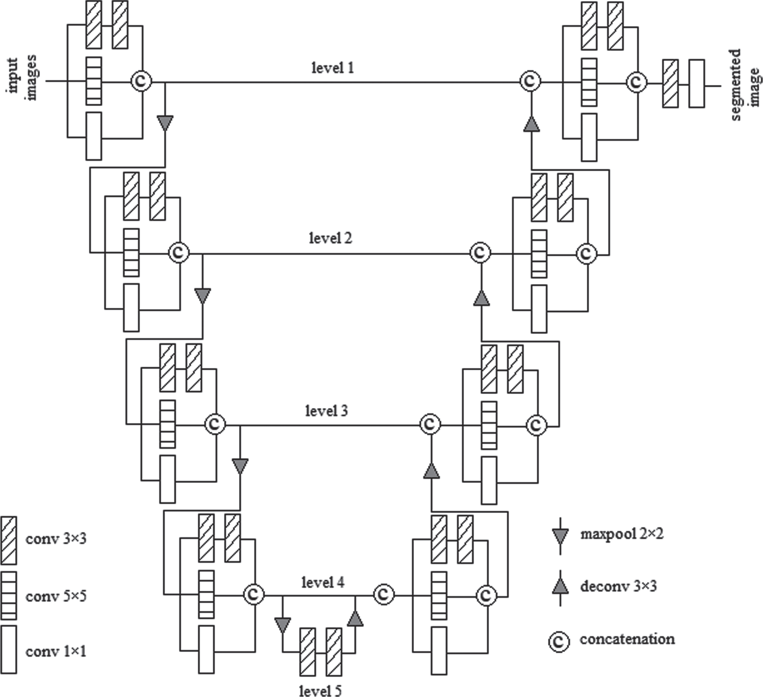
Modified inception module based U-Net (IMU-Net) architecture.

The decoder block of all levels consists of a concatenation of the preceding level upsampling output and the encoder block IM output of the same level. The IM follows the concatenation output on each level. The Feature channels are reduced as half using upsampling operation. The entire decoder block maximizes the spatial dimensions and minimizes the channels. The last decoder block IM output is feed into 64 kernels, and the final layer holds a sigmoid activation to classify tumors and background.

3.4 Modified inception module

The IM is a general block for levels 1 to 4 of the proposed IMU-Net model. The IM in the proposed model is the concatenation of two series 3×3 kernels, one 5×5, one 1×1 convolution kernels. The layer arrangement and kernel size of IM have shown in Fig. 3.

Fig. 3

Inception module.

The two sequences 3×3 convolution kernel in IM having some filters = [64, 128, 256, 512, 1024] for levels 1 to 5 respectively, and 5×5, 1×1 convolution kernels have numbers of filters = [32, 64, 128, 256] for levels 1 to 4 respectively. The depth of IM decreases with a 1×1 small convolution kernel and local features extracted from the 3×3 convolution kernel and generic features collected from the 5×5 convolution kernel. Among these convolution kernels, 1×1 kernel makes single point convolution, and 3×3 kernel deals with 9 pixels in an image and 5×5 kernels deal with 25 pixels in an image. Maxpool operation follows IM in encoder block, and IM follows upsampling operation in decoder block. Level 5 has concatenation of two series 3×3 convolution kernels without 5×5 and 1×1 convolution kernels.

In the encoder block, level 1 gets the initial shape of [240, 240, 4] MR image as an input has fed into IM, which produces output shape [240, 240, 128]. The subsequent maxpool layer creates [120, 120, 128] feature maps, then given to IM of level 2. It generates output shape [120, 120, 256]. The subsequent maxpool layer gives [60, 60, 256] feature maps, then fed into IM of level 3. It generates output in the shape of [60, 60, 512]. The subsequent maxpool layer generates [30, 30, 512] feature map shapes, then fed into IM of level 4. It produces output in the shape of [30, 30, 1024]. The following maxpool layer provides [15, 15, 1024] the shape of feature maps and feeds into level 5.

In the decoder path, the upsampling of level 5 yields a shape [30, 30, 512] feature maps. Level 4 has concatenation of preceding level 5 outputs and encoder block level 4 IM outputs which have a shape [30, 30, 1536]. The subsequent IM generates output in the shape of [30, 30, 1024]. [60, 60, 256] feature maps are created by upsampling level 4 outputs. Level 3 is the concatenation of upsampling level 4 outputs and encoder block level 3 outputs that have a shape [60, 60, 768]. The subsequent IM yields output with the shape [60, 60, 512]. The upsampling level 3 output has a shape [120, 120, 128]. Level 2 has concatenation of preceding upsample level 3 outputs and encoder block level 2 IM outputs, and it yields the shape [120, 120, 384]. The subsequent IM generates output with the shape of [120, 120, 256]. The upsampling of level 2 outputs create the shape [240, 240, 64]. Level 1 has concatenation of preceding upsample level 2 outputs and encoder block level 1 output, and it yields the shape [240, 240, 192]. The subsequent IM generates output with the shape of [240, 240, 128]. The preceding output [240, 240, 128] has followed by one hidden convolution layer, and then the final convolution layer with a 1x1 kernel produces the segmented output image in the shape of [240, 240, 1].

4 Implementation

This section illustrates the Dataset preparation, model configuration, and the training details.

4.1 Dataset

The proposed model selects a dataset from Medical Image Computing and Computer-Assisted Invention (MICCAI) and Brain Tumor Segmentation (BraTS) challenge. The BraTS 2017 training dataset has 285 training data (210 HGG and 75 LGG), where 50 HGG volumes and 12 LGG volumes are given randomly to a model. The shape of the MR image is [240, 240, 155], and each volume consists of 155 slices. The proposed model gets slices from 55 to 115 because the remaining slices do not contain useful information. The training dataset consists of four modalities FLAIR, T1, T1ce, T2, and labeled data for all subjects. T1 and T2 images are the most common MRI sequences. Cerebrospinal fluid (CSF) distinguishes T1 and T2 MRI sequences easily. T1 imaging has a dark spot on CSF, and T2 imaging has a bright spot on CSF. In the Flair sequence, CSF is dark like the T1 sequence but bright on abnormal tissues. The difference between CSF and abnormality is easy to find on the Flair sequence, and Flair is very sensitive to pathology. The T1 sequence infusion of Gadolinium (Gad) enhancement agent is beneficial in looking at tumor structures [40]. These four MRI input sequences are supplied into the proposed model to get WT, CT, and ET. The same proposed model has trained to get WT, CT, and ET effectively. The Ground truth result of the training dataset holds four labels namely;

Healthy pixel (Label ‘0’)

A Necrotic and non-enhance tumor (Label ‘1’)

Edema (Label ‘2’)

Enhance tumor (Label ‘4’)

From the above labels, Necrotic is the dead tissue which causes due to little blood or no blood supply to the brain tissue. High radiation, head injuries are the causes of a necrotic tumor. The non-enhancing tumor is commonly available in LGG. It represents a large portion of the whole tumor in the Flair sequence [40]. Label ‘1’ in the dataset has the combination of necrotic and non-enhanced tumors. In edema, the skull gets pressure when CSF flow increases around the brain. Label ‘2’ in the dataset has edema or brain swelling. Edema causes a reduction of the oxygen flow in the brain. It occurs in a part of the brain or entire brain that causes death if not treated. Gad agent highlights the affected lesions during active inflammation. The T1 weighted contrast-enhanced MRI sequence [13] has the highlighted aggressive lesion potion. It is called an enhanced tumor. Label ‘4’ in the dataset has the enhanced tumor. WT is a combination of labels 1, 2, 4. CT is a combination of labels 1, 4, and ET is labeled 4. The images from the dataset are free from noise, and it is skull stripped.

4.2 Model configurations

The proposed IMU-Net model has chosen Adam optimizer, dice loss as a cost function, DSC, and IOU as the evaluation metrics. The most preferred metrics for medical image segmentation are DSC and IOU. Generally, DSC performs similarity measures between Ground truth and predicted results. DSC has a value in the range of 0 (no match) to 1 (perfect match). DSC is well suited for class imbalance problems, and it deals with a large number of background voxels. IOU gives overlap between two samples. It is in the range of 0 to 1. Identical or complete overlap sample regions give 1, and no overlap sample regions give 0. It is highly dependent on the intersection zones. It measures successively when the input is sparse data. A Good model has higher DSC and IOU values. The main objective of the optimizer is to reduce the cost function value. The Adam optimizer belongs to the adaptive optimizer family. So, the learning rate has auto-tuned in the training stage. It takes the benefits of RMSprop, Adadelta optimizers and yields better results for sparse gradients in noisy environments. Table 1 gives the configuration parameters of the Adam optimizer, and these default values [11] give efficient results for computer vision applications using deep learning. The step size closer to zero gives an optimum value. Hence, the initial step size, 3e-06 selected to provide the optimum result for the proposed model. In Adam optimizer, the parameter vector update rules [11] have given in Eqs. (5) where β₁ is an exponential decay of the first momentum, β₂ is an exponential decay of the second momentum, ɛ is a small value to avoid divide by zero error, g_t is gradient value, and α is the learning rate. The relu activation function detects features faster and performs the model in a better direction. The final layer of the model carries the sigmoid activation function to distinguish tumors and the background of an image. It has attained with Google’s colab notebook, TensorFlow framework, and TensorLayer [15] library.

Table 1
Configuration parameters of Adam optimizer

S.No Proposed Model Adam Optimizer parameters

β₁ β₂ α ɛ

1. IMU-Net 0.9 0.999 3e-06 1e-08

S.No	Proposed Model	Adam Optimizer parameters
1.	IMU-Net	0.9	0.999	3e-06	1e-08

$θ_{t + 1} = θ_{t} - \frac{α}{\sqrt{{\hat{υ}}_{t} + ɛ}} {\hat{m}}_{t}$ (1)

The bias corrected first momentum ${\hat{m}}_{t}$ and bias corrected second momentum ${\hat{υ}}_{t}$ are given as, ${\hat{m}}_{t} = \frac{m_{t}}{1 - β_{1}^{t}}$ (2) ${\hat{υ}}_{t} = \frac{υ_{t}}{1 - β_{2}^{t}}$ (3)

The biased first momentum m_t and biased second momentum υ_t are given as, $m_{t} = β_{1} . m_{t - 1} + (1 - β_{1}) g_{t}$ (4) $υ_{t} = β_{2} . υ_{t - 1} + (1 - β_{2}) g_{t}^{2}$ (5)

4.3 Training details

The BRATS 2017 training dataset has unnormalized data that have different pixel intensity values. This high variance scaled data has a high impact on an error while training a model. So, the images from the dataset are given into Z-score normalization [12] to provide normalized data. The normalized data has a standard deviation close to 1 and a mean value close to 0. It has randomly partitioned into training and validation sets in the ratio of 80 : 20 from the 50 HGG and 12 LGG volumes. Both training set and validation set get HGG and LGG volumes after partition. The data augmentation process gets normalized data and produces eight various samples for each subject. The new dataset following the augmentation process is divided into batches where every batch consists of 5 images. The mini-batches reduce the computational cost, and it holds less memory. The normalization and eight distinct augmentation images of one subject with all MRI sequences have shown in Fig. 4. The input shape of the deep learning model is [5, 240, 240, 4], where the batch size is 5, 2D image shapes are [240, 240], and the number of MRI sequences is 4. The output shape of the deep learning model is [5, 240, 240, 1], where the tumor type is specified by 1. The proposed model has trained separately to get WT, CT, and ET. The non-differentiable DSC and IOU are used to measure the similarity between ground truth and predicted results. The evaluation metrics Hard DSC and Hard IOU had mentioned in Eqs. (7), where Ygt^t is the ground truth with the threshold value 0.5 and Yseg^t is the predicted result with the threshold value 0.5. Dice loss is the best choice to deal with an imbalanced dataset [6, 27]. It had measured from the soft DSC, and it is immune to an imbalanced dataset. Equation (8) gives Dice loss computation, where Ygt is the ground truth result without threshold, and Yseg is the predicted result without threshold.

Fig. 4

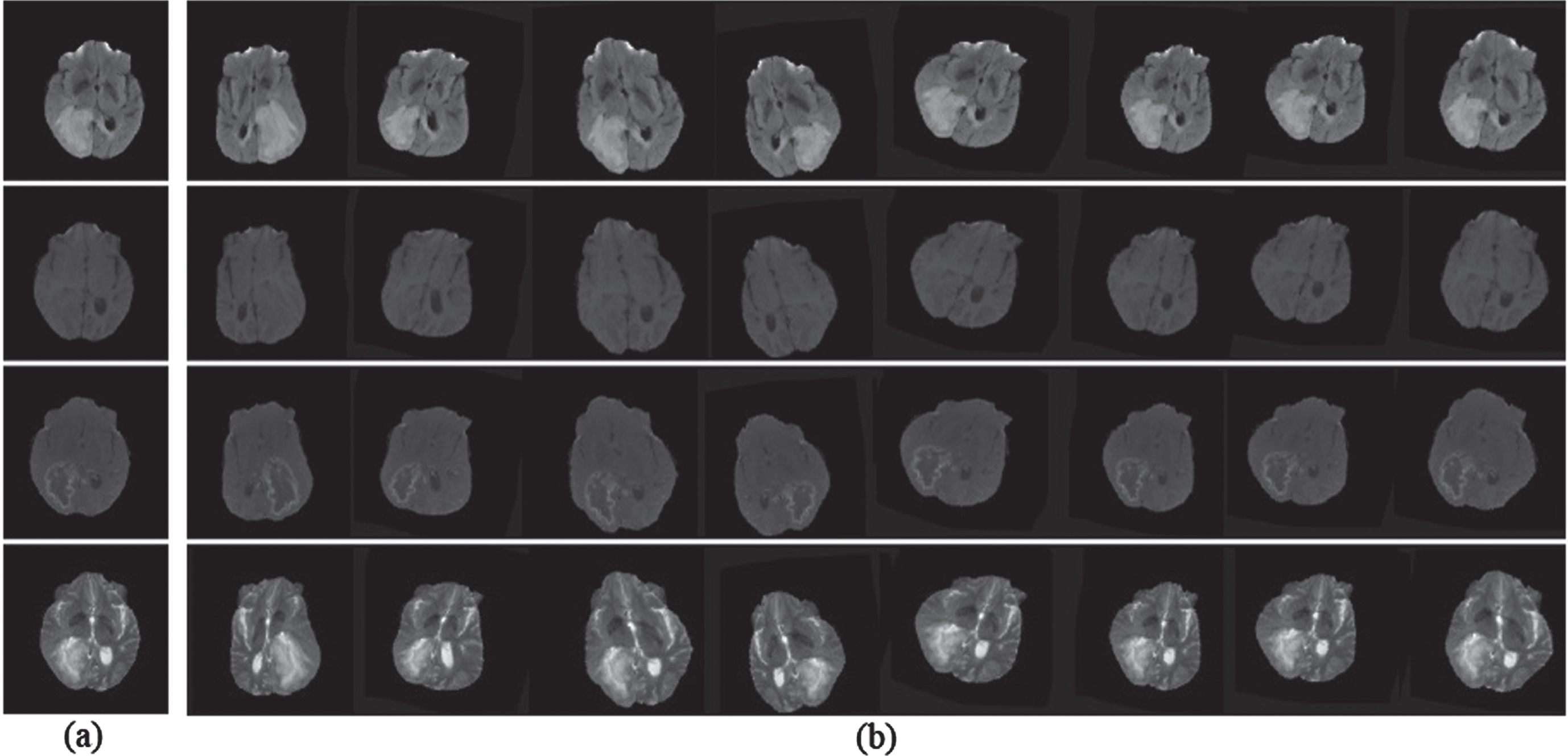
Flair, T1, T1ce, and T2 MRI sequences of (a) Normalized image, (b) Augmented image.

$DSC = \frac{2 ({Ygt}^{t} \cap {Yseg}^{t})}{{Ygt}^{t} + {Yseg}^{t}}$ (6) $IoU = \frac{{Ygt}^{t} \cap {Yseg}^{t}}{{Ygt}^{t} \cup {Yseg}^{t}}$ (7) $Dice loss = 1 - \frac{2 (Ygt \cap Yseg)}{Ygt + Yseg}$ (8)

5 Results and discussion

Triple cascaded DNN structure [41] comprises three sequence models viz WNet, TNet, and ENet. The original training images have cropped into 96×96×96×1 to eliminate unwanted background data. The testing phase is different from the training phase; the last layer follows an additional post-processing task to avoid misclassified tumors in the testing phase. The segmented image has a dimension of 96×96×96×2. WNet receives an input image which provides WT, and WT has passed into TNet, which provides TC, and TC has passed into ENet, which provides ET. The sequence models provide DSC as 0.90, 0.78, and 0.83 for WT, CT, and ET during the evaluation. A CNN [25] model contains the training phase and testing phase separately. Training images have 4×33×33 patches where the channels are 4. The final fully connected (FC) layer produces a segmented image in the shape of 5×1×1, which classifies five different tumor sub-regions. The CNN model has competed in BRATS 2015 challenges and obtains DSC as 0.78, 0.65, and 0.75 for WT, CT, and ET. The dropout regularization follows the maxpool layer to avoid overfitting towards a model. In the SegNet [1] model, both the encoder and decoder blocks have 13 convolution layers, and the last layer in the decoder path has a multi-class softmax activation function. The cropped image of shape 192×192×3 is generated from the original image to eliminate unwanted black parts of an image and reduces memory. The cropping data is fed into a model and generates segmented image 192×192×4. During the evaluation, the SegNet model gives DSC as 0.85, 0.81, and 0.79 for WT, CT, and ET using BRATS 2017 dataset.

A two-path CNN network [16] obtains local features from the local path and global context from the global path. Training images had divided into 4×33×33 patches where the channels are 4. The final layer of the model is a fully connected layer that produces a segmented image in the shape of 5×1×1, where it classifies five different tumor sub-regions. A local path is similar to the conventional CNN structure, and the aforementioned two-path CNN provides DSC as 0.85, 0.78, and 0.73 for WT, CT, and ET. The nested residual attention blocks (NRAB) [35] model contain an encoder path, decoder path, and skip connection. The NRAB has the input in the dimension of 240×240×4. The final layer predicts the multi-label classifications, which provide the output in the shape of 240×240×5. It furnishes DSC as 0.87, 0.80, and 0.72 for WT, CT, and ET. BU-Net [28] is a modified U-Net structure, and it has two modules; the Residual extended skip (RES) module and the Wide context (WC) module. The RES module creates middle-level features from the low-level features and the sub-regions of tumors classified by the WC module. BU-Net gets input MR image in the shape of 256×256×4 and gives segmented output in the dimension of 256×256×6. It provides DSC as 0.89, 0.78, and 0.73 for WT, CT, and ET during evaluation by using the BRATS 2017 dataset.

Table 2 presents a detailed comparison of the proposed method with existing methods. During an evaluation, the proposed model attains a mean DSC of 0.90, 0.77, and 0.74 for WT, CT, and ET, and a mean IOU of 0.79, 0.70, and 0.70 for WT, CT, and ET. IOU metric not investigated with existing methods [1 , 41]. IOU provides overlap between the predicted tumor regions and ground truth tumor regions. Data augmentation process not investigated with few existing methods [1 , 41]. The proposed model IMU-Net and WNet [41] are the best models for WT compared to other existing methods. SegNet and ENet [41] are the best models for CT and ET, respectively. Fig. 5 depicts the DSC and IOU of the proposed model for each epoch. Dice loss predicts a mismatch between prediction result and ground truth result. The predicted probabilities of the samples compared with ground truth samples without a threshold and binary conversion. The weights and biases are optimized based on the dice loss to obtain a good fit model. The cost function for each epoch has shown in Fig. 6, which decreases during evaluation. The Dice loss for WT, CT, and ET is reduced during training and stops at 0.09, 0.24, and 0.23. The training progress has halted before it becomes overfit. The ground truth and predicted output of one subject has shown in Fig. 7. The first row has WT, the second row has CT, and the third row has ET of Ground truth and predicted output using the proposed model. Existing methods were estimated using the DSC metric, whereas the proposed method uses DSC and IOU metrics for evaluation. It achieved better results than other existing methods. Finally, a physician makes a treatment plan based on the tumors such as WT, CT, and ET, other factors such as the patient’s age, health condition, tumor location, and size. Generally, treatment plans like surgery, radiation therapy, and chemotherapy decide by physicians concerning said conditions.

Table 2
Investigation on proposed model with existing methods

S.No Methods Input Output DSC IOU

WT CT ET WT CT ET

1 Proposed model 5×240×240×4 5×240×240×1 0.9 0.77 0.74 0.79 0.7 0.7

2 Wang et al. [41] 96×96×96×1 96×96×96×2 0.9 0.78 0.83 _ _ _

3 Pereria et al. [25] 4×33×33 5×1×1 0.78 0.65 0.75 _ _ _

4 Havaei et al. [16] 4×33×33 5×1×1 0.85 0.78 0.73 _ _ _

5 Sun et al. [35] 240×240×4 240×240×5 0.87 0.8 0.72 _ _ _

6 Alqazzaz et al. [1] 192×192×3 192×192×4 0.85 0.81 0.79 _ _ _

7 Rehman et al. [28] 256×256×4 256×256×6 0.89 0.78 0.73 _ _ _

S.No	Methods	Input	Output	DSC	IOU
1	Proposed model	5×240×240×4	5×240×240×1	0.9	0.77	0.74	0.79	0.7	0.7
2	Wang et al. [41]	96×96×96×1	96×96×96×2	0.9	0.78	0.83	_	_	_
3	Pereria et al. [25]	4×33×33	5×1×1	0.78	0.65	0.75	_	_	_
4	Havaei et al. [16]	4×33×33	5×1×1	0.85	0.78	0.73	_	_	_
5	Sun et al. [35]	240×240×4	240×240×5	0.87	0.8	0.72	_	_	_
6	Alqazzaz et al. [1]	192×192×3	192×192×4	0.85	0.81	0.79	_	_	_
7	Rehman et al. [28]	256×256×4	256×256×6	0.89	0.78	0.73	_	_	_

Fig. 5

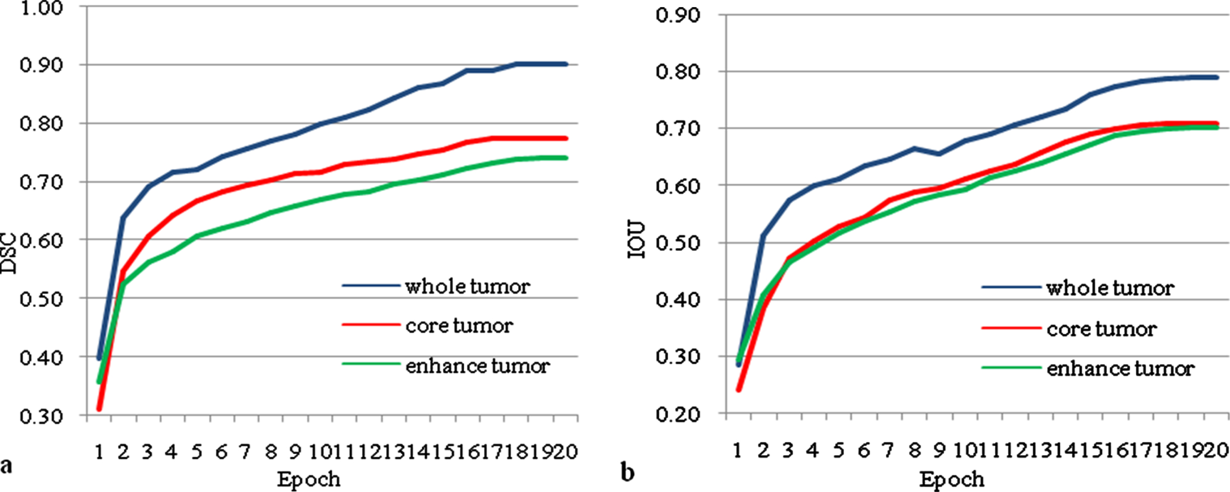
(a) Dice similarity co-efficient (DSC), (b) Intersection over union (IOU) of the proposed model IMU-Net Vs epoch.

Fig. 6

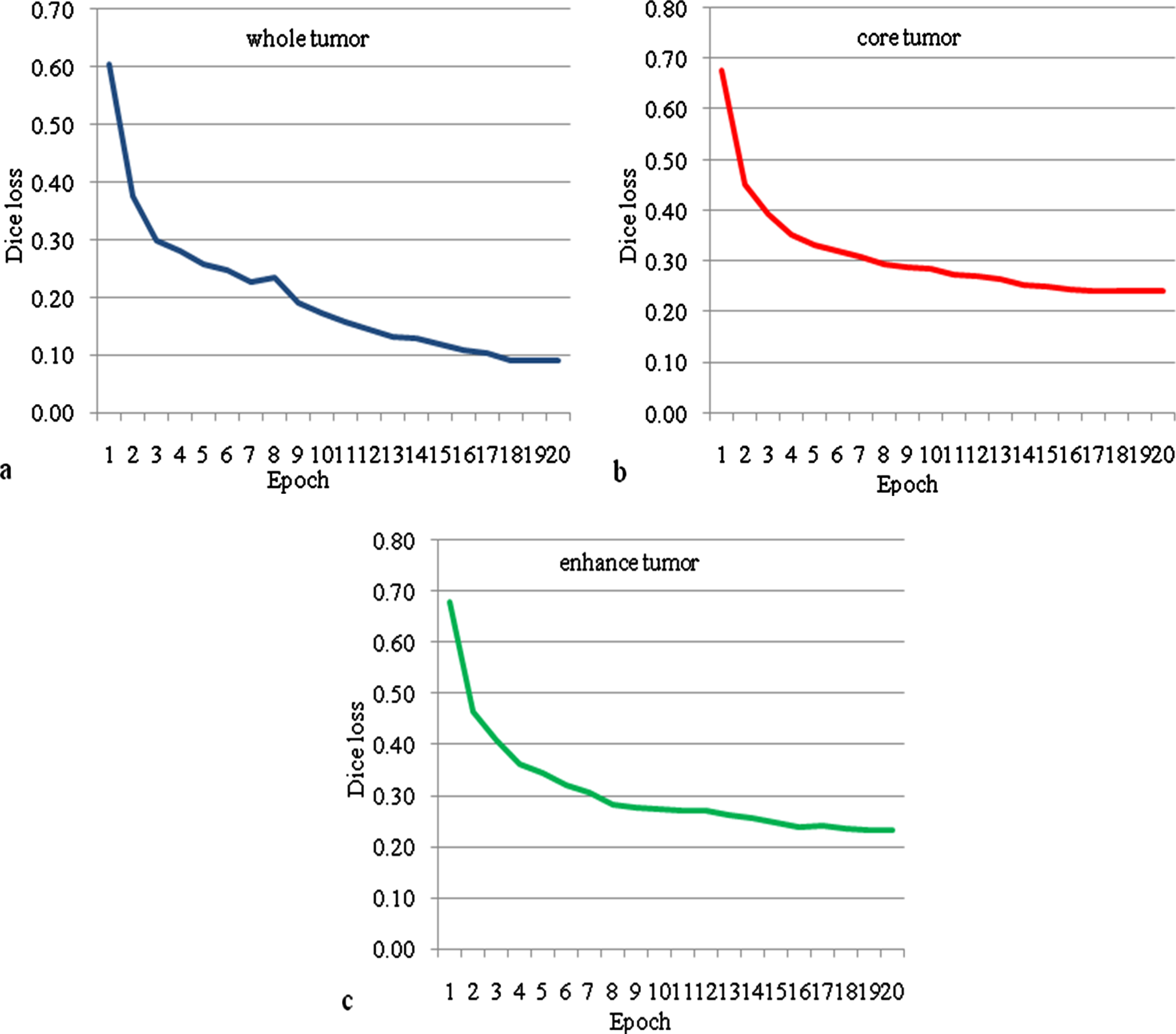
Dice loss of the proposed model IMU-Net for (a) whole tumor, (b) core tumor, (c) enhance tumor Vs epoch.

Fig. 7

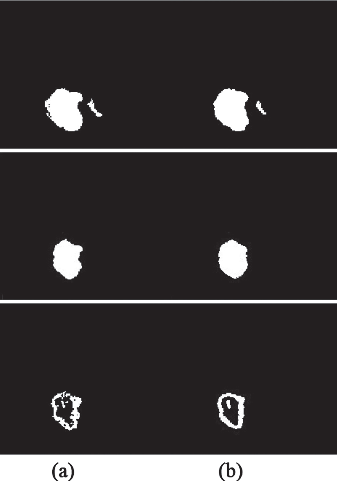
(a) Ground truth, (b) Predicted output of Whole tumor (WT), Core tumor (CT), and Enhance tumor (ET).

6 Conclusion

The proposed model has divided into three sub-tasks: data normalization, data augmentation, and tumor segmentation. The proposed model includes 36 convolution layers and four deconvolution layers. It has 63.59 million training parameters and takes 520 minutes approximately to train a model. The number of training parameters is less compared to existing deep learning methods. The proposed model utilizes the advantages of extracting features at a different scale of the modified inception module (IM). It gets local features, global context from U-Net architecture and reduces dice loss. It provides better segmentation results compared to existing methods for the WT. In the future, adapt with the different methodologies, improves segmentation results for CT and ET.

References

Alqazzaz

, Sun

, Yang

, et al., Automated brain tumorsegmentation on multi-modal MR image using SegNet, Comp Visual Media 5 (2019), 209–219. https://doi.org/10.1007/s41095-019-0139-y.

Vishnuvarthanan

, Pallikonda Rajasekaran

, Govindaraj

, Zhang

and Thiyagarajan

, An Automated Hybrid Approach Using Clustering and Nature Inspired Optimization Technique for Improved Tumor and Tissue Segmentation in Magnetic Resonance Brain Images, Applied Soft Computing Journal. https://dx-doi-org.web.bisu.edu.cn/10.1016/j.asoc.2017.04.023.

Menze

B.H.

, et al., The Multimodal Brain Tumor Image Segmentation Benchmark (BRATS),”, in IEEE Transactions on Medical Imaging 34(10) (2015), 1993–2024. doi:10.1109/TMI.2014.2377694.

Bakas

, Akbari

, Sotiras

, et al., Advancing the Cancer Genome Atlas glioma MRI collections with expert segmentation labels and radiomic features, Sci Data 4 (2017), 170117. https://doi.org/10.1038/sdata.2017.117.

Banerjee

, Mitra

, Masulli

and Rovetta

, Brain Tumor Detection and Classification from Multi-sequence MRI: Study Using Conv Nets, In: A. Crimi, S. Bakas, H. Kuijf, F. Keyvan, M. Reyes, T. van Walsum, (eds) Brainlesion: Glioma, Multiple Sclerosis, Stroke and Traumatic Brain Injuries, BrainLes 2018. Lecture Notes in Computer Science, vol 11383, 2019. Springer, Cham. https://doi.org/10.1007/978-3-030-11723-8_17.

Bertels

, et al., Optimizing the Dice Score and Jaccard Index for Medical Image Segmentation: Theory and Practice. In: Shen D. et al., (eds) Medical Image Computing and Computer Assisted Intervention –MICCAI 2019, MIC-CAI 2019. Lecture Notes in Computer Science, vol 11765, Springer, Cham. https://doi.org/10.1007/978-3-030-32245-8_11.

Szegedy

, et al., Going deeper with convolutions, 2015 IEEE Conference on Computer Vision and Pattern Recognition (CVPR), Boston, MA, USA, 2015, pp. 1–9. doi: 10.1109/CVPR.2015.7298594.

Zhou

, Ding

, Wang

, Lu

and Tao

, One-Pass Multi-Task Networks With Cross-Task Guided Attention for Brain Tumor Segmentation, in IEEE Transactions on Image Processing, vol. 29 (2020), pp. 4516–4529. doi: 10.1109/TIP.2020.2973510.

Chalela

J.A.

, Kidwell

C.S.

, Nentwich

L.M.

, Luby

, Butman

J.A.

, Demchuk

A.M.

, Hill

M.D.

, Patronas

, Latour

and Warach

, Magnetic resonance imaging and computed tomography in emergency assessment of patients with suspected acute stroke: a prospective comparison, Lancet 369(9558) (2007), 293–298 10.1016/S0140-6736(07)60151-2PMID: 17258669; PMCID: PMC1859855.

10.

Chen

, Bentley

, Mori

, Misawa

, Fujiwara

and Rueckert

, DRINet for Medical Image Segmentation, IEEE Trans Med Imaging 37(11) (2018), 2453–2462. doi:10.1109/TMI.2018.2835303. Epub 2018 May 10. PMID: 29993738.

11.

Kingma

D.P.

and Ba

, Adam: A method for stochastic optimization, arXiv: 1412.6980, (2014). https://arxiv.org/abs/1412.6980.

12.

Ellingson

B.M.

, Zaw

, Cloughesy

T.F.

, Naeini

K.M.

, Lalezari

, Mong

, Lai

, Nghiemphu

P.L.

and Pope

W.B.

, Comparison between intensity normalization techniques for dynamic susceptibility contrast (DSC)-MRI estimates of cerebral blood volume (CBV) in human gliomas, J Magn Reson Imaging 35 (2012), 1472–1477. https://doi.org/10.1002/jmri.23600.

13.

Giorgio

, Stromillo

M.L.

, Bartolozzi

M.L.

, et al., Relevance of hypointense brain MRI lesions for long-term worsening of clinical disability in relapsing multiple sclerosis, Multiple Sclerosis Journal 20(2) (2014), 214–219. doi: 10.1177/1352458513494490.

14.

Hanif

, Muzaffar

, Perveen

, Malhi

S.M.

and Simjee

, Sh, Glioblastoma Multiforme: A Review of its Epidemiology and Pathogenesis through Clinical Presentation and Treatment, Asian Pacific Journal of Cancer Prevention: APJCP 18(1) (2017), 3–9. doi: 10.22034/apjcp.2017.18.1.3.

15.

Dong

, Supratak

, Mai

, Liu

, Oehmichen

, Yu

and Guo

, TensorLayer: A Versatile Library for Efficient Deep Learning Development, In Proceedings of the 25th ACM international conference on Multimedia (MM ’17). Association for Computing Machinery, New York, NY, USA, 2017, 1201–1204. doi: https://doi.org/10.1145/3123266.3129391.

16.

Havaei

, Davy

, Warde-Farley

, Biard

, Courville

, Bengio

, Pal

, Jodoin

P.M.

and Larochelle

, Larochelle, Brain tumor segmentation with Deep Neural Networks, Med Image Anal 35 (2017), 18–31. doi: 10.1016/j.media.2016.05.004. Epub 2016 May 19. PMID: 27310171.

17.

Ibtehaz

and Rahman

M.S.

, MultiResUNet: Rethinking the U-Net architecture for multimodal biomedical image segmentation, Neural Netw 121 (2020), 74–87. doi: 10.1016/j.neunet.2019.08.025. PMID: 31536901.

18.

, Wang

, Kong

, et al., Hypergraph membrane system based F 2fully convolutional neural network for brain tumor segmentation, Applied Soft Computing Journal (2020), doi: https://doi.org/10.1016/j.asoc.2020.106454.

19.

Kamnitsas

, Ledig

, Newcombe

, Simpson

J.P.

, Kane

, Menon

, Rueckert

and Glocker

, Efficient multiscale 3D CNN with fully connected CRF for accurate brain lesion segmentation, 2017. doi: 10.17863/CAM.6936.

20.

Kistler

, Bonaretti

, Pfahrer

, Niklaus

and Büchler

, The virtual skeleton database: an open access repository for biomedical research and collaboration, . Published Nov, J Med Internet Res 15(11) (2013), e245. Published 2013 Nov 12.10.2196/jmir.2930.

21.

Kociołek

, Strzelecki

and Obuchowicz

, Does image normalization and intensity resolution impact texture classification? Comput Med Imaging Graph 81 (2020), 101716. doi: 10.1016/j.compmedimag.2020.101716. Epub 2020 Mar 6. PMID: 32222685.

22.

Lim

, Kim

and Cheon

, A Deep Neural Network-Based Method for Early Detection of Osteoarthritis Using Statistical Data, International Journal of Environmental Research and Public Health, 16(7) (2019), 1281. https://doi.org/10.3390/ijerph16071281.

23.

Louis

D.N.

, Perry

, Reifenberger

, et al., The World Health Organization Classification of Tumors of the Central Nervous System: a summary, Acta Neuropathol 131 (2016), 803–820. https://doi.org/10.1007/s00401-016-1545-1.

24.

Mittal

, Goyal

L.M.

, Verma

, Kaur

and Hemanth

D.J.

, Deep learning based enhanced tumor segmentation approach for MR brain images, Applied Soft Computing 78 (2019), 346–354.

25.

Pereira

, Pinto

, Alves

and Silva

C.A.

, Brain Tumor Segmentation Using Convolutional Neural Networks in MRI Images, IEEE Trans Med Imaging 35(5) (2016), 1240–1251. doi: 10.1109/TMI.2016.2538465. Epub 2016 Mar 4. PMID: 26960222.

26.

Punn

N.S.

and Agarwal

, Multi-modality encoded fusion with 3D inception U-net and decoder model for brain tumor segmentation, Multimed Tools Appl, (2020). https://doi.org/10.1007/s11042-020-09271-0.

27.

Zhao

, et al., Rethinking Dice Loss for Medical Image Segmentation, 2020 IEEE International Conference on Data Mining (ICDM), 2020, pp. 851&860. doi: 10.1109/ICDM50108.2020.00094.

28.

Rehman

M.U.

, Cho

, Kim

J.H.

and Chong

K.T.

, BU-Net: Brain Tumor Segmentation Using Modified U-Net Architecture, Electronics, 9(12) (2020), 2203.. https://doi.org/10.3390/electronics9122203.

29.

Riaz

and Hashmi

M.R.

, Linear Diophantine Fuzzy Set and Its Applications Towards Multi-attribute Decision-making Problems, 1 Jan. 2019:5417–5439.

30.

Ronneberger

, Fischer

and Brox

, U-Net: Convolutional Networks for Biomedical Image Segmentation, In: Navab N., Hornegger J., Wells W., Frangi A. (eds) Medical Image Computing and Computer-Assisted Intervention –MICCAI 2015. MICCAI 2015. Lecture Notes in Computer Science, vol 9351, 2015, Springer, Cham. https://doi.org/10.1007/978-3-319-24574-428

31.

Liu

and Deng

, Very deep convolutional neural network based image classification using small training sample size, 2015 3rd IAPR Asian Conference on Pattern Recognition (ACPR), 2015, pp. 730–734, doi: 10.1109/ACPR.2015.7486599.

32.

Sajid

, Hussain

and Sarwar

, Brain Tumor Detection and Segmentation in MR Images Using Deep Learning, Arab J Sci Eng 44 (2019), 9249–9261. https://doi.org/10.1007/s13369-019-03967-8.

33.

Sladojevic

, Arsenovic

, Anderla

, Culibrk

and Stefanovic

, Deep Neural Networks Based Recognition of Plant Diseases by Leaf Image Classification, Computational Intelligence and Neuroscience, vol. 2016, Article ID 3289801, 11 pages, 2016. https://doi.org/10.1155/2016/3289801.

34.

Srinivas

and Sasibhushana

, Rao, Segmentation of Multi-Modal MRI Brain Tumor Sub-Regions Using Deep Learning, J Electr Eng Technol 15 (2020), 1899–1909. https://doi.org/10.1007/s42835-020-00448-z.

35.

Sun

, Li

and Liu

, Semantic segmentation of brain tumor with nested residual attention networks, Multimed Tools Appl, (2020). https://doi.org/10.1007/s11042-020-09840-3.

36.

Sun

, Zhang

, Chen

and Luo

, Brain Tumor Segmentation and Survival Prediction Using Multimodal MRI Scans With Deep Learning, Front Neurosci 13 (2019), 810. doi: 10.3389/fnins.2019.00810.

37.

Taylor

O.G.

, Brzozowski

J.S.

and Skelding

K.A.

, Glioblastoma Multiforme: An Overview of Emerging Therapeutic Targets, Front Oncol 9 (2019), 963. doi: 10.3389/fonc.2019.00963. PMID: 31616641; PMCID: PMC6775189.

38.

Thillaikkarasi

and Saravanan

, An Enhancement of Deep Learning Algorithm for Brain Tumor Segmentation Using Kernel Based CNN with M-SVM, J Med Syst 43(4) (2019), 84. doi: 10.1007/s10916-019-1223-7. PMID: 30810822.

39.

Tong

, Zhang

, Weng

, et al., Kernel sparse representation for MRI image analysis in automatic brain tumor segmentation, Frontiers Inf Technol Electronic Eng 19 (2018), 471–480. https://doi.org/10.1631/FITEE.1620342.

40.

Upadhyay

and Waldman

A.D.

, Conventional MRI evaluation of gliomas, (Spec No 2, Spec Iss 2), The British Journal of Radiology 84 (2011), S107–S111. doi: 10.1259/bjr/65711810.

41.

Wang

, Li

, Ourselin

and Vercauteren

, Automatic Brain Tumor Segmentation Using Cascaded Anisotropic Convolutional Neural Networks, (2018). 10.1007/978-3-319-75238-9_16.

42.

Wang

, Feng

, Bu

, Cui

, Xie

, Zhang

, Feng

, Zhu

and Chen

, MDU-Net: A Convolutional Network for Clavicle and Rib Segmentation from a Chest Radiograph, Journal of Healthcare Engineering, vol. 2020 (2020), 9, Article ID 2785464. https://doi.org/10.1155/2020/2785464.

43.

Song

, Ji

, Sun

and Zheng

, A Novel Brain Tumor Segmentation from Multi-Modality MRI via A Level-Set-Based Model, J Signal Process Syst 87(2) (2017), 249–257. doi: https://doi.org/10.1007/s11265-016-1188-4.

An automatic brain tumor segmentation using modified inception module based U-Net model

Abstract

Keywords

1 Introduction

2 Related work

3 Methodology

3.1 Data pre-processing

3.3 Deep neural network

4.1 Dataset

4.2 Model configurations

Table 1 Configuration parameters of Adam optimizer S.No Proposed Model Adam Optimizer parameters β1 β2 α ɛ 1. IMU-Net 0.9 0.999 3e-06 1e-08

References

Table 1
Configuration parameters of Adam optimizer

S.No Proposed Model Adam Optimizer parameters

β₁ β₂ α ɛ

1. IMU-Net 0.9 0.999 3e-06 1e-08