An efficient hexagonal image framework using pseudo hexagonal pixel for computer vision applications

Abstract

Nature-inspired computing has been a real source of motivation for the development of many meta-heuristic algorithms. The biological optic system can be patterned as a cascade of sub-filters from the photoreceptors over the ganglion cells in the fovea to some simple cells in the visual cortex. This spark has inspired many researchers to examine the biological retina in order to learn more about information processing capabilities. The photoreceptor cones and rods in the human fovea resemble hexagon more than a rectangular structure. However, the hexagonal meshes provide higher packing density, consistent neighborhood connectivity, and better angular correction compared to the rectilinear square mesh. In this paper, a novel 2-D interpolation hexagonal lattice conversion algorithm has been proposed to develop an efficient hexagonal mesh framework for computer vision applications. The proposed algorithm comprises effective pseudo-hexagonal structures which guarantee to keep align with our human visual system. It provides the hexagonal simulated images to visually verify without using any hexagonal capture or display device. The simulation results manifest that the proposed algorithm achieves a higher Peak Signal-to-Noise Ratio of 98.45 and offers a high-resolution image with a lesser mean square error of 0.59.

Keywords

Computer vision Nature Inspired Computing hexagonal image color image Human Visual System

1 Introduction

In the fast-growing field of computer science and technology, natural computing has become a promising solution for upcoming researchers. Nature Inspired Computing (NIC) has inspired from the natural world led to many innovative algorithms and computations [1]. To bring a revolution in the application of computer vision, many extensive works are progressed in the hexagonal tessellation lattice. NIC methods are more flexible, robust, fast deliverable, easily understandable, and adaptable. Consequently, it is utilized to solve a broad range of computations and applications.

In order to replicate the characteristics of the Human Visual System (HVS), it is very significant that the spatial arrangement of machine vision sensors should be arranged based on the arrangement of high-density cones and rods in the human fovea. Nevertheless, today’s practical world adopts rectangular meshes rather than hexagonal meshes due to the ease of hardware implementation, availability, and familiarity with the cartesian coordinate system. There is a strong connection of hexagonal geometry with the human visual system as hexagonal pixels fit the shape of human fovea [2] as illustrated in Fig. 1. Moreover, the hexagonal lattice has typically seen in nature such as beehives, dragonfly eyes, bubble rafts, etc., [3].

Fig. 1

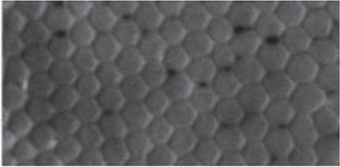
Photoreceptor cons and rods in human fovea.

A brief description of how the picture is taken by the human eye is as follows. On the posterior portion of the eye, the retina is a thin membrane (or tissue). The major aim of the retina is to capture the light data and transform them into neural signals that can be sent to the brain for further visual processing. The fovea is a small retinal area whose structure comprises highly dense hexagonal-shaped rods and cones that are placed on a hexagonal grid. This kind of spatial arrangement in hexagonal lattice provides added advantage over the square lattice when it comes to detecting straight and circular edges with higher accuracy [4].

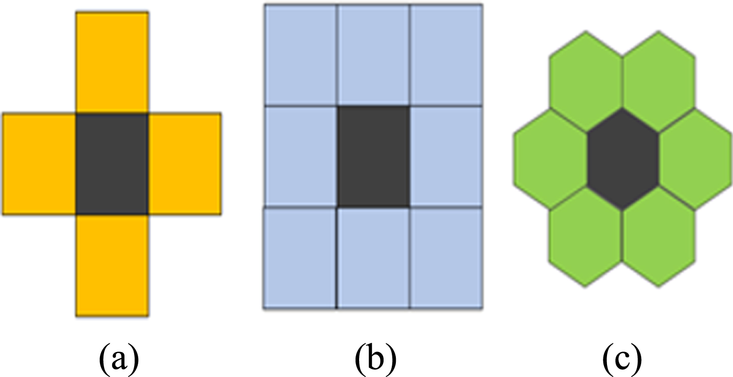
Given a 2-D image, in many instances, it is of a prominent challenge to build up a spatial domain structure that resembles HVS to achieve a real-time performance [5]. Rectilinear square mesh is generally used in camera sensors and display screens due to its ease of implementation in the cartesian coordinate systems and its orthogonal nature. But wherever the symmetric geometric computation between contiguous neighboring pixels is required, the square mesh does not satisfy this requirement. Even though commercially dedicated machinery visual sensors are trying to approximate photoreceptor densities seen in primate retinas, they can’t still reach and outperformed by HVS in terms of the wide range and the processing capabilities at the sensor level. This stimulus has given rise to the recent research about biological retinas to collect more information regarding the processing strategies with the ray of hope to the design and development of ideal visual sensors [6]. In practice, various lattice systems are accessible such as squares, triangles, and hexagons [7] as depicted in Fig. 2. These tessellation schemes allow us to tile a plane without any overlap and vacant spaces between them. All other spatial arrangements of tessellation will follow an uneven distance between neighborhood pixels and overlap between samples.

Fig. 2

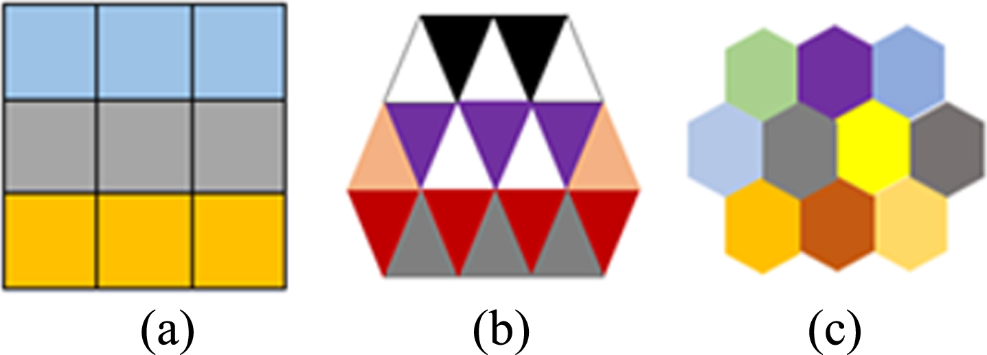
Common tessellation schemes a) square b) triangle c) hexagon.

Figure 2 a) illustrates the most common and simple tessellation that aligns with the cartesian coordinate system. Figure 2 b) is the triangular tessellation which is having a higher packing density than the square tessellations. Figure 2 c) is the hexagonal tessellation which is regarded to be the most efficient tessellation scheme that aligns with the HVS. It has many geometrical advantages like consistent neighbourhood pixels, higher packing density, equidistant neighbourhood connectivity, and better angular correction. Furthermore, the additional benefit of this geometric arrangement is derived from human anatomical thought of the primate’s perspective [8].

On the 2-D image frame, the image forms a group of hexagonal pixels, and this arrangement results in the sharp vision for capturing information. In addition to imitating the characteristics of the human retina, the hexagonal grid comprises other geometrical advantages such as the representation of curved structures more accurately, equidistance to the neighbouring pixels, and improved spatial isotropy for the efficient implementation of circular kernels which leads to the increase in accuracy when detecting both curved and straight edges [9]. Hexagonal architecture has arranged in a set of 7 hexagons whereas conventional square architecture exhibits 3×3 matrix units as demonstrated in Fig. 3.

Fig. 3

Pixel architecture a) hexagon b) square.

The cartesian coordinate system can address only traditional square lattice images only. Hence, the hexagonal grid image system needs a proper coordinate system for efficient addressing and storing the data. Different dominant addressing schemes to deal with the hexagonal structure are two –axes oblique coordinate addressing scheme [10, 11], three–coordinate symmetrical coordinate frame, and a single indexing scheme as shown in Fig. 4.

Fig. 4

Addressing schemes a) two-axes oblique b) three coordinates symmetrical *R³ c) relationship between *R³ and R³ d) single indexing-spiral architecture.

Using a two-axis oblique coordinate system, an ordered pair of vectors is employed to represent each hexagonal pixel in both horizontal and vertical direction as depicted in Fig. 4a. This system has the following advantages: (i) Complete - In 2-D space, a point can be represented efficiently and accurately; (ii) Unique - An exact ordered pair coordinates can be assigned to a point representation; (iii) Convertible - It is similar to the cartesian coordinate system and can be easily transformed to and from the co-ordinate system. In [12], the three-axis coordinate frame has been introduced and is also referred to as a symmetrical hexagonal coordinate frame. This coordinate frame uses three coordinates x, y, z as shown in Fig. 4b, and there exists a one-to-one mapping of a symmetrical hexagonal frame (*R³) and three-dimensional cartesian frames (R³) as shown in Fig. 4c. Any three-pixel coordinates follow the relationship which is given by Equation (1). The distance between the neighbouring pixel is unit distance. $x + y + z = 0$ (1)

Owing to the close and adjacent relationship between symmetrical hexagonal coordinate frame and three-dimensional, all geometrical transformation and theoretical explanation can be conveniently transferred to and from *R³ to R³. The structural symmetry property can be efficiently preserved in this scheme.

Spiral addressing is another way to represent the hexagonal structure based on a Hexagonal Discrete Fourier Transform (HDFT) method [13]. Hexagonal pixels are arranged in spiral clusters where each pixel having consistent 6 neighbouring pixels. The basic step in spiral addressing is the numbering each hexagon with a unique address from the middle of the image in raised powers of seven in a spiral curve pattern as shown in Fig. 4d. Primarily, the address has been applied to a group of 7 hexagons labelled consecutively like 0, 1, 2, 3, 4, 5, and 6.

As illustrated in Fig. 5, the structure can be dilated to place additional 6 hexagons consecutively and each address is multiplied by 10. For each newly installed hexagon, an address will be provided with respect to the centre pixel address as performed for the first seven hexagons. After that, the hexagons numbered form the cluster of size 7ⁿ (n = 1, 2, 3, . . .). A one-dimensional addressing scheme with a collection of 49 pixels is exposed in Fig. 4d. This architecture provides an additional benefit of fixing the centre of the image at the origin and consistent 6-neighbourhood connectivity which is helpful for numerous computer vision applications.

Fig. 5

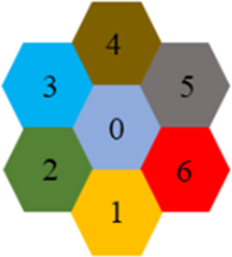
Cluster of basic seven hexagonal cells.

In this paper, 2-axes oblique co-ordinate system has been exploited to simulate the hexagonal grid. It will effectively make use of existing hardware implementation. The major outperforming contribution of this paper is as follows:

A new 2-D Interpolation Hexagonal Lattice Conversion (2IHLC) algorithm has been developed to attain an effective hexagonal mesh framework. This framework design will be employed for several image processing and computer vision applications.

An appropriate development of pseudo-hexagonal structure in the proposed 2IHLC algorithm yields a better peak signal-to-noise ratio, and a lesser mean square error.

More than 98%of the pixel contributes to the pseudo-hexagonal structure framework simulation and higher resolution images are obtained in the proposed 2IHLC algorithm.

The organization of this research article is as adhered. Section 2 summarizes the literature description of hexagonal image processing. Section 3 describes the hexagonal image lattice, representation, and processing. Section 4 states the proposed 2IHLC algorithm. The results and discussions are demonstrated in Section 5. Finally, Section 6 deals with a conclusion and all possible future work.

2 Related works

While there are obvious advantages of using hexagonal images, the dearth of the utilization of hexagonal lattice is mostly attributable to the inadequacy of hardware devices, including both sensors for collecting hexagonal images and devices for displaying them. In order to continue research advancements in this technology using the existing hardware, there is a need to build an effective resampling strategy so that we can benefit from the advantages that hexagonal lattice offers for the processing of images.

The Linear Hexagonal Resampling (LHR) technique can be determined to make it ready for display and processing using existing hardware devices [14]. The pixels in a real hexagonal structure are not organized in a spiral pattern. Instead, various addressing schemes and coordinate systems are introduced to simulate hexagonal grids [15, 16]. In this section, the details of hexagonal sampling and numerous resampling methodologies are illuminated to enable the conversion of square lattice to the hexagonal grid.

2.1 Hexagonal sampling

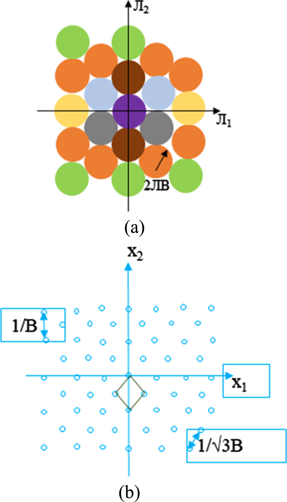
According to [17], a rectangular space sampling is not desirable because it has many disadvantages, such as spatial resolution varying with direction. As a result, the best sampling pattern will be a normal hexagonal pattern. Hexagonal sampling is considered as the best sampling scheme for signals that are band-limited over a circular region of the Fourier plane since the exact reconstruction of the waveform requires a lower sampling density than alternative schemes as shown in Fig. 6. For such signals, the hexagonal sampling use 13.4%fewer samples than rectangular sampling.

Fig. 6

Different sampling schemes a) rectangular sampling b) hexagonal sampling.

$x (n_{1}, n_{2}) = x_{a} (n_{1} T_{1}, n_{2} T_{2})$ (2) where x_a (T₁, T₂) represents the analog image, T₁ and T₂ signify the sampling intervals in the horizontal and vertical direction, x (n₁, n₂) denotes the rectangular sampled sequence. Let x_a (Ω₁, Ω₂)designates the Fourier transform of x_a (T₁, T₂). If it satisfies the condition: x_a (Ω₁, Ω₂) = 0, (Ω₁, Ω₂) R, then the image is signified as band-limited as exposed in Fig. 6a. Further, the image can be exactly reconstructed using Equation (3). $T_{1} < \frac{π}{w_{1}} and T_{2} < \frac{π}{w_{2}}$ (3) where W₁ and W₂ intend the horizontal and vertical bandwidth respectively. Hexagonal sampling can be represented in a similar way to rectangular sampling and it is expressed as. $x (n_{1}, n_{2}) = x_{a} (\frac{2 n_{1} - n_{2}}{2} T_{1}, n_{2} T_{2})$ (4) where x (n₁, n₂) represents the hexagonally sampled image as shown in Fig. 6b. In order to exactly recover the original image, it should be band-limited with a hexagonal band region through Equation (5). $T_{1} ⩽ \frac{4 π}{2 w_{1} + w_{2}} and T_{2} ⩽ \frac{π}{w_{2}}$ (5)

2.2 Resampling methodology

a)Alternate Pixel Suppressed (APS) Method

According to [18], the hexagonal grid upon rectangular grid can be obtained by alternatively vanquishing horizontal rows and vertical columns of the pre-existing rectangular grid. The equation for sub-sampling is as follows: ${pixel}_{{val}_{hex (i, j)}} = {\begin{matrix} {pixel}_{val (2 * i, 2 * j)}, if is even \\ {pixel}_{val (2 * i, 2 * j + 1)}, if i is odd \end{matrix}$ (6)

In this method, there is no one-to-one correspondence between the pixels in the hexagonal grid and rectangular grid as some of the pixels are suppressed. Zero values are assigned to the suppressed pixels. While doing the computations with the sub-sampled images, the suppressed pixels are not taken into account. Therefore, new sampled images have only a quarter of a pixel compared to a rectangular grid as depicted in Fig. 7.

Fig. 7

Mesh formation a) rectangular mesh b) sub-sampled hexagonal mesh.

b) Half-Pixel Shift (HPS) Method

The HPS method has been introduced to addresses the hexagonal lattice issues like imperfect hexagonal shape, lower intensity, and smaller resolution [19]. It is evaluated by applying the overlaps strategy between square and hexagonal pixels where these overlaps are framed mathematically using 8 separate circumstances. Every overlap scenario has sensed automatically and utilized to calculate the final hexagonal intensity. For each odd line, the midpoint is computed through simple interpolation equation (i.e., mid = (left _value + right _value)/2), discarding the left-most and right-most values, retaining only mid-point values. The hexagonal mapping equation is as follows: $p^{new} (x, 2 y) = p^{old} (x, 2 y)$ (7)

$\begin{matrix} p^{new} (x, 2 y + 1) \\ = \frac{p^{old} (x, 2 y + 1) + p^{old} (x + 1, 2 y + 1)}{2} \end{matrix}$ (8)

3 Features of hexagonal sampling scheme

The hexagonal sampling scheme offers several features as compared with existing schemes. Some of them are as follows:

3.1 More efficient sampling scheme

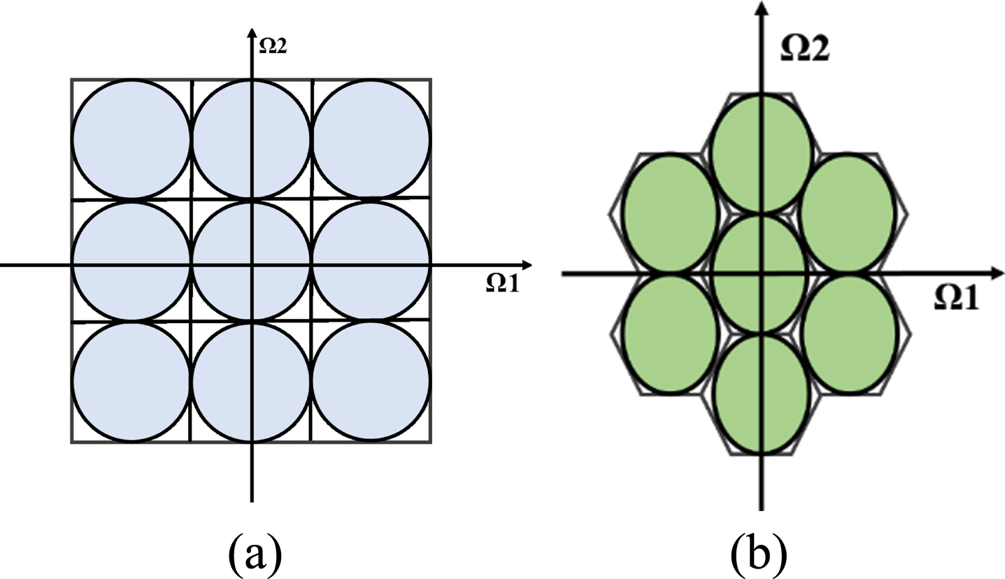
Aliasing is referred to as a process of insufficient sampling rate which leads to undesirable effects in the recovered signal. In [20], they investigated the fact that lesser samples are necessary for the regeneration of wave number limited input signal in hexagonal grid. Using this, the fundamental inference is that, the square lattice is not an efficient sampling scheme. Consequently, when using the 2-D isotropic function, the rhombic hexagon (120⁰) is considered as an effective sampling lattice as illustrated in Fig. 8. Here, the spacing between the sampling points is given by $\frac{1}{\sqrt 3 * B}$ and the spectrum is bounded by circles with radius 2πB as shown in Fig. 8a and 8b.

Fig. 8

Sampling lattice for a) circular function b) isotropic function.

3.2 Smaller quantisation error

Quantization error is a vital parameter to calculate the merit of the layout of different available sensors. The authors in [21, 22] developed an equation for calculating quantization error in hexagonal sampling lattice and proved that lesser quantization error can be achieved in comparison to square sampling lattice as depicted in Fig. 9.

Fig. 9

Spectral packaging for a) square and b) hexagonal.

3.3 Consistent connectivity

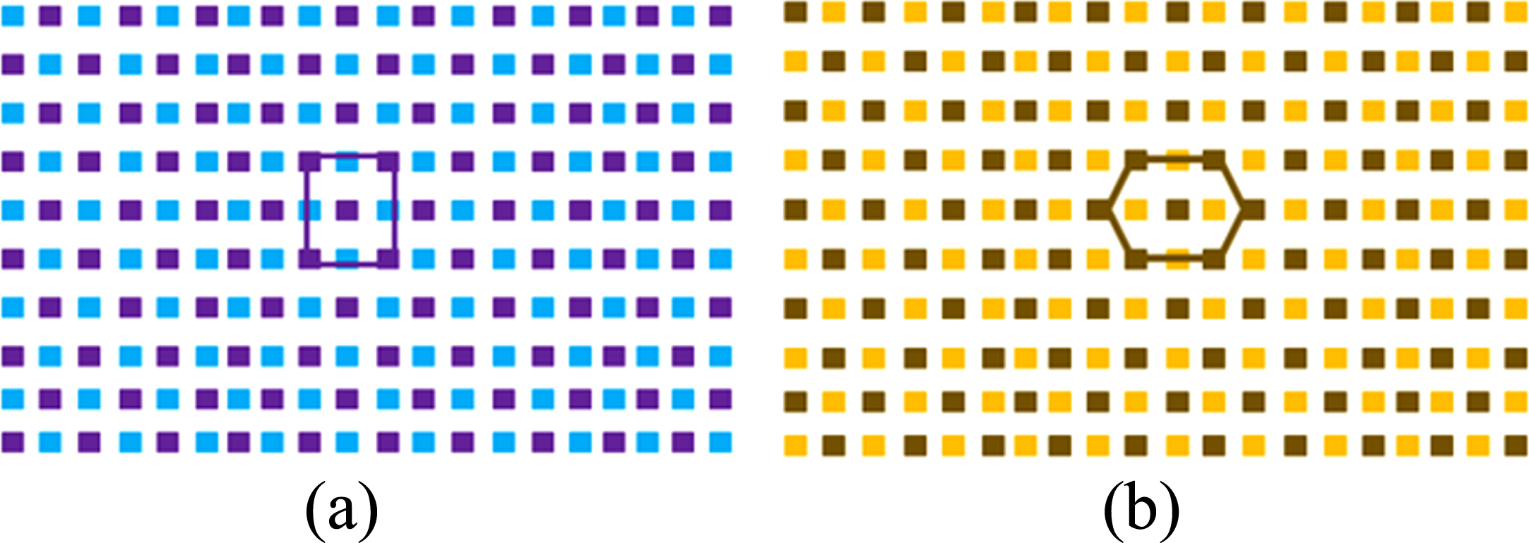
One of the fundamental concepts in digital image processing is the connectivity between the pixels. Two pixels are said to be connected, if they are neighbours and if they satisfy the specified condition of similarity [23]. In the case of a square grid, there is two-pixel neighbourhood. We consider the pixels are connected if they share a common edge or when they possess a common corner.

Accordingly, the square grid is having 4-neighbourhood and 8-neighbourhood pixels as illustrated in Fig. 10a and 10b. But in the case of the hexagonal grid, there is no choice of connectivity [24, 25]. We can define only, 6-neighbourhood connectivity and the neighbouring pixel share only one common edge and two common corners as illustrated in Fig. 10c. Due to the unavailability of choice of connectivity, many image processing as well as computer vision algorithms can be easily and efficiently implemented. The neighbourhood connectivity for the hexagonal grid is consistent and fixed to 6-way connectivity.

Fig. 10

Neighbouring pixels in (a,b) square lattice, (c) hexagonal lattice.

3.4 Equidistance

In the conventional square lattice image, there are two different types of distance measures are taken into account [26 –28]. The distance calculated between the adjacent pixels in the diagonal orientations is √2 times the corresponding horizontal orientation as shown in Fig. 11a. In the hexagonal grid, every hexagon is having consistent 6 neighbours and all are equidistant from the centre pixel along the six sides of the pixel as represented in Fig. 11b. Due to these features, the hexagonal sampling will be considered in the proposed 2IHLC algorithm and it is explained in the following section.

Fig. 11

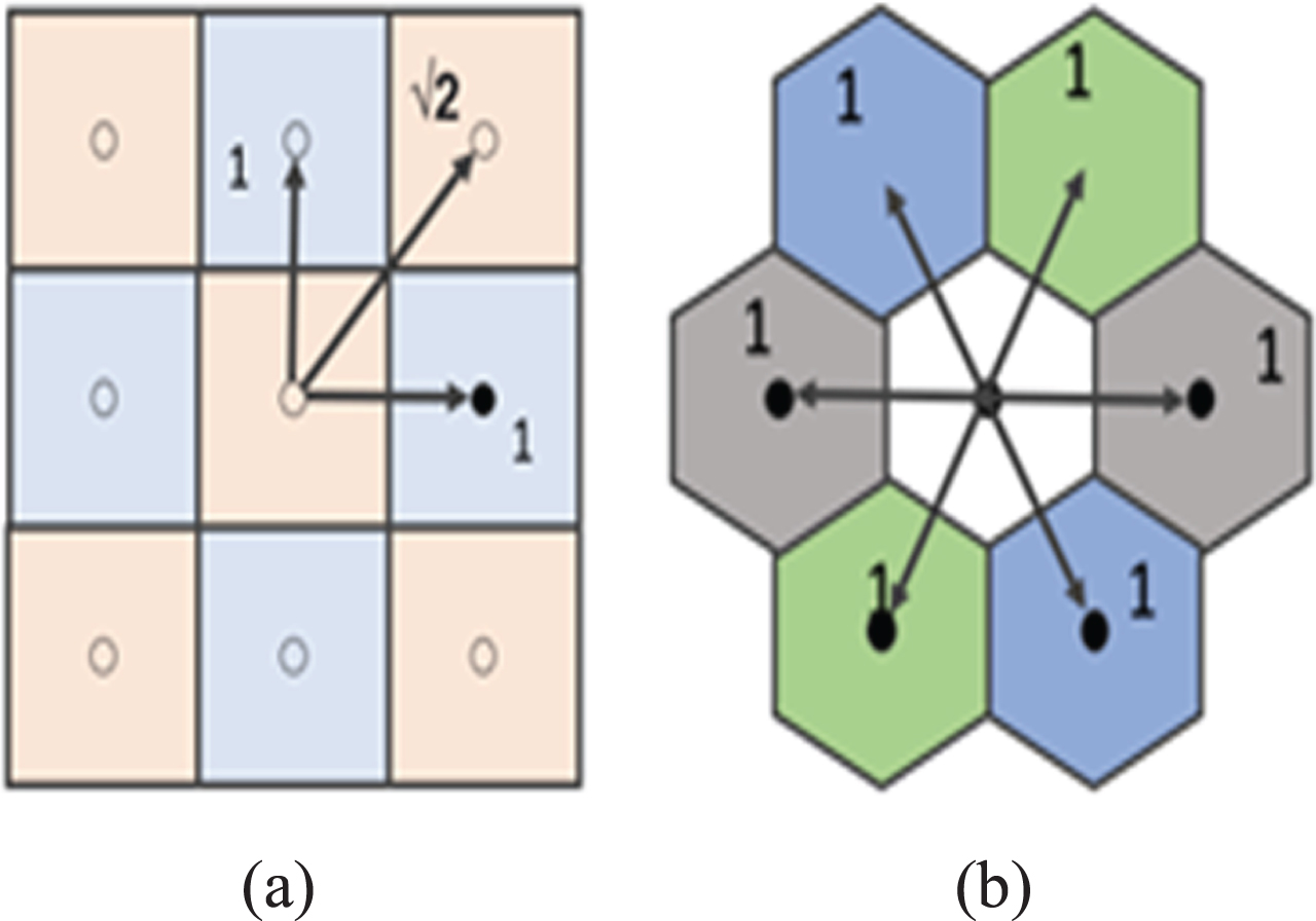
Distance measure for a) square b) hexagon.

4 Proposed 2IHLC Methodology

The resampling as well as conversion of square latticed images to hexagonal latticed image is mandatory in proposed 2IHLC algorithm. In this new technique, each pixel is represented by a n × n pixel block. The sub-pixel hexagonal image is employed for processing of image in virtual hexagonal environment. The flow of converting the square grid image into hexagonal grid image with the aid of proposed algorithm is depicted in Fig. 12. It utilizes the benefit of hexagonal image processing that can be directly used in the today’s world, where it lacks the availability of hexagonal image sensors.

Fig. 12

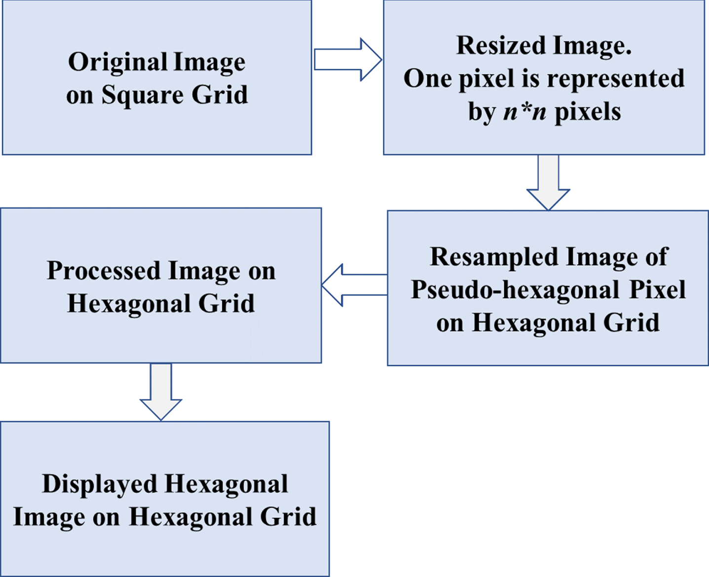
Processing of hexagonal images in proposed method.

Sub-pixel clustering effect is produced in the resampling process, which limits the loss of resolution effect. A 6×6 block of pixels represents each hexagonal pixel. Selection of the number of pixels that form the hexagonal pixel is collected separately and it is focused on two policy issues such as:

Arrangement of pixels should allow tessellation extraction without overlap and there are no gaps between the six-dimensional neighbours pixels;

Collection of pixels should resemble hexagons. For instance, Hexagonal pixel lattice should adhere to the properties of the geometry.

4.1 Hexagonal Pixel Simulation

Hexagonal image simulation in proposed method is typically achieved by resampling rectilinear square pixel centred images using pseudo software simulation. From a group of square sub-pixels, the proposed algorithm generates hexagonal pixels where each pixel is represented by n × n pixel block in order to enable the sub-pixel clustering and attain same resolution. For example, in Fig. 13, each pixel of the given image is represented by a 6×6-pixel block with same intensity as that of the original square grid image is used for the construction of hexagonal image. Square pixels which are used to create six pixels labelled as ‘1’ with the remaining pixels labelled as ‘0’ discarded.

Fig. 13

Hexagonal pixel arrangement from square pixel.

All square pixels in the input image can be transformed to hexagonal pixels using this method. Further, all hexagonal pixel clusters are arranged on the square grid as exposed in Fig. 14. The pixel-coloured yellow shows first row first column A (1,1) and pixel-coloured green implies first row first column A (1,2). Similarly, all the pixels are numbered like above where A represents the hexagonal structured image.

Fig. 14

Collection of hexagonal pixels.

Algorithm 1

Proposed 2IHLC Algorithm
Step 1: Start
Step 2: Read the image in any format
(jpg,bmp,*png)
Step 3: Extract the shape of the image.
Step 4: Define a zero matrix of size 6×6.
Step 5: Select the pixel positions marked 1 and fill
it with corresponding pixel intensity values.
Step 6: Create a bigger zero matrix which is 6 times
the size of the image.
Step 7: Fill the corresponding positions with the
corresponding intensity values.
Step 8: Perform left and up shifting by calculating
the pixel values needed to be shifted.
Step 9: Do the shifting till the pixels align correctly
with the neighbourhood pixels.
Step 10: Get the hexagonal structured image.
Step 11: End

The complete square pixels can be converted to pseudo hexagonal pixels through Algorithm 1. It utilizes a 2-axes oblique coordinate system that follows the row-column addressing so that we can make use of existing hardware to process the image. The row-column addressing in the proposed 2IHLC algorithm follows in a similar way to the familiar Cartesian coordinate system. Besides, the proposed method of hexagonal pixel simulation can also be employed on colour images.

As the colour image consists of three channels, the proposed algorithm should be applied two-three (RGB) channels separately and superimpose these results. The proposed hexagonal grid possesses the same symmetry in 0⁰, 60⁰, and 120⁰. This higher symmetry makes many image processing and computer vision applications more beneficial. For example, if the images are rotated on a hexagonal grid, more information of the image will be retained by the proposed 2IHLC algorithm when compared with the square grid.

5 Results and discussions

The effectiveness of the proposed 2IHLC algorithm has been evaluated in the Python platform and its system specification is demonstrated in Table 1. The performance of the proposed method is compared with the HDFT [13], LHR [14], APS [18], and HPS [19] methods in terms of Peak Signal-to-Noise Ratio (PSNR), Average Information Content (AIC), Mean Square Error (MSE), Average Running Time (ART), and Contrast Enhancement Index (CEI).

Table 1
System Specification

Simulation Tool Python 3.8

Operating System Windows 7 (64 bit)

RAM 8GB RAM

Processor Intel premium

Dataset Lena.jpg and Fruits.jpg

Image size 32×32, 64×64, 128×128, 225×225, 512×512

Simulation Tool	Python 3.8
Operating System	Windows 7 (64 bit)
RAM	8GB RAM
Processor	Intel premium
Dataset	Lena.jpg and Fruits.jpg
Image size	32×32, 64×64, 128×128, 225×225, 512×512

The comparative performance of these methods is enumerated in Table 2. To ensure that the comparisons were fair, all the methods have a similar network models as well as mapping strategies. Figure 15 and Figure 16 demonstrate the grey-scale image and color image with pseudo-hexagonal pixels simulated using the proposed 2IHLC algorithm. The pseudo hexagonal pixels can be seen in the zoomed view. Lena.jpg and fruits.jpg of different sizes are utilized for the proposed algorithm and verified.

Table 2

Comparitive Analysis of Different Methods

Methods	Percentage of Pixels Used	Image Enhancement Filters	Boundary of the Image	Image Central Position	Neighbouring Pixel
HDFT	60.25	Zero-order hold reconstruction filter	Hexagonal	Top-left corner	Hexagonal
LHR	45.00	Linear filter	Hexagonal	Centre	Hexagonal
APS	50.00	Gabor filter	Square	Top-left corner	Square
HPS	70.83	Gabor filter	Square	Top-left corner	Square
Proposed 2IHLC method	98.89	No filter	Hexagonal	Centre	Hexagon

Fig. 15

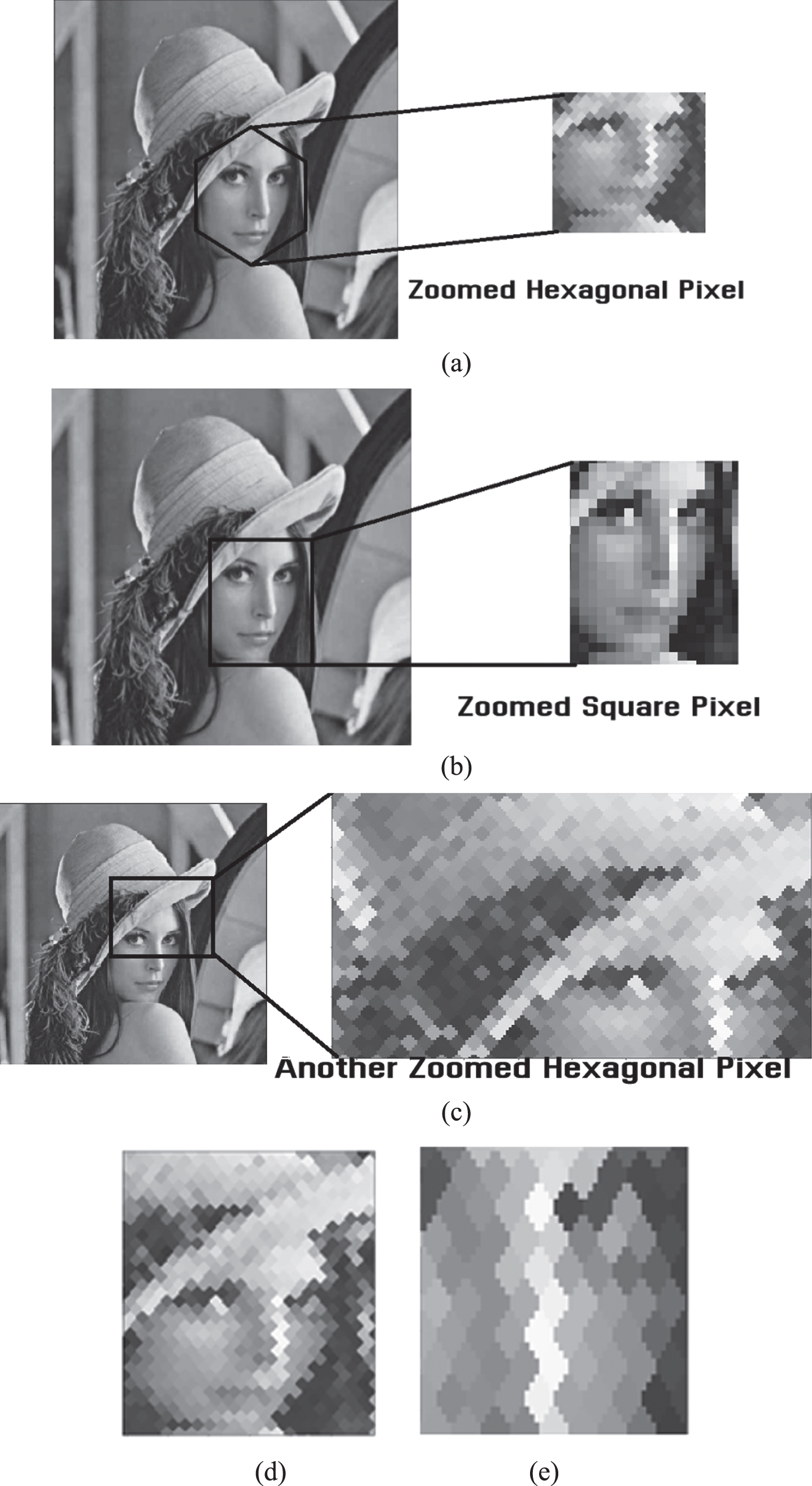
Simulation results of grey scale image uing proposed algorithmn a) with hexagonal pixels b) with square pixels c) another zoomed version of hexagonal pixels d) and e) higher zoomed version of hexagonal pixels.

Fig. 16

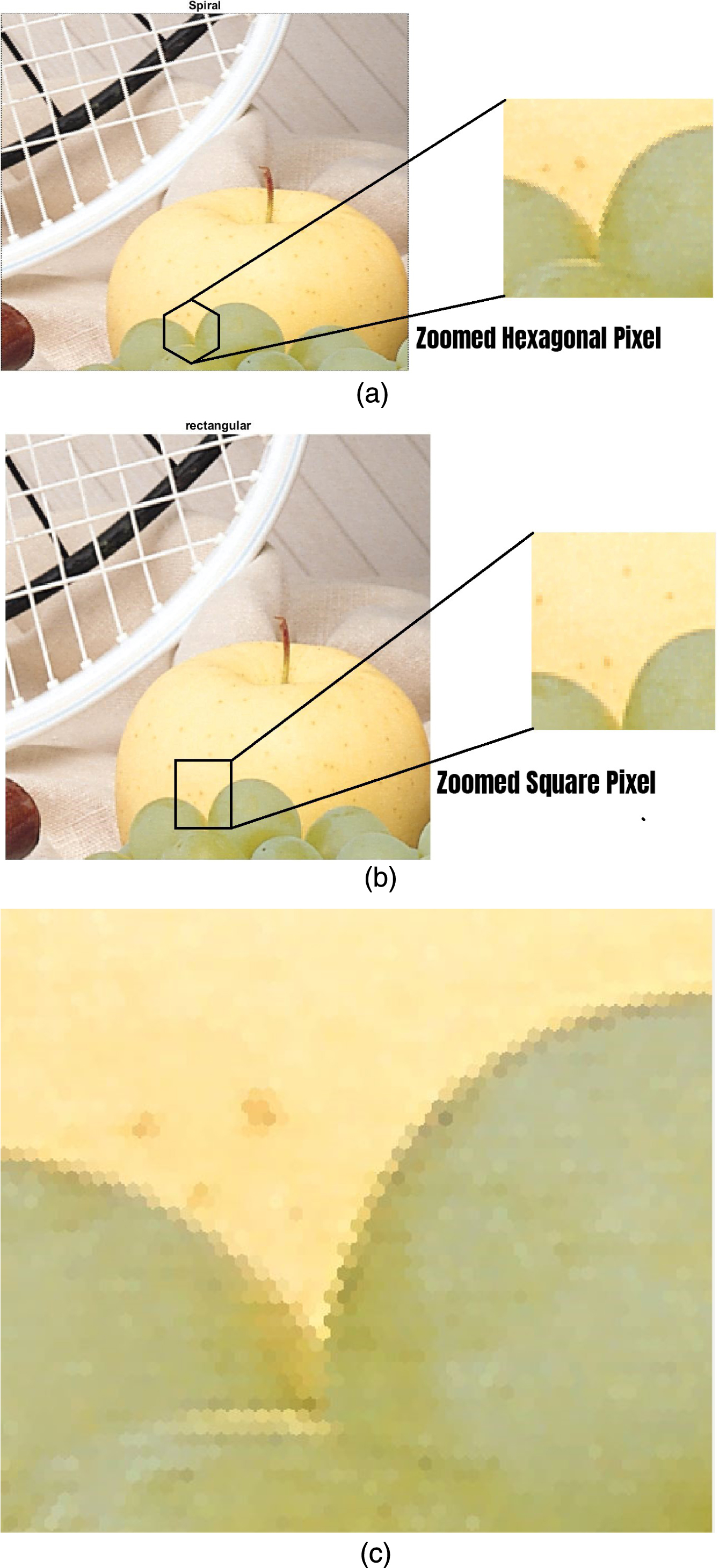
Simulation results of color image using proposed algorithmn a) with hexagonal pixels b) with square pixels c) zoomed view of hexagonal pixels.

From the Fig. 15 16, it is evident that the images simulated by the proposed algorithm provide equidistant, consistent connectivity pixels and high-resolution images. This is owing to the execution of efficient pseudo software simulation in the proposed 2IHLC method. It utilizes a 2-axes oblique coordinate system which follows the row-column addressing to process the image. Besides, the formation of hexagonal structure pixel in the proposed 2IHLC method follows high symmetric property where this higher symmetry makes many image processing and computer vision applications more beneficial.

5.1 Performance Analysis of PSNR

Typically, the input images are utilized for simulation may be corrupted owing to noise and hence the evaluation of PSNR is required to quantify the presence of noise in the image. PSNR can be expressed as follows: $PSNR = 10 {log}_{10} [\frac{N \times 255^{2}}{\sum_{i} \sum_{j} {(X_{ij} - V_{ij})}^{2}}]$ (9) where N implies the size of the image, X denotes the hexagonal processed image, and V indicates the original input image.

According to Fig. 17, it is evident that the proposed 2IHLC method yields a higher PSNR value as compared with existing methods under varying image sizes. In particular, the proposed 2IHLC still acquires with 96.8 PSNR value at the larger grey-scale image, whereas the HDFT method obtains 80 PSNR value only. The PSNR value of 2IHLC has enhanced by 14%, 13%, 11%, and 8%as compared to HDFT, LHR, APS, and HPS methods respectively.

Fig. 17

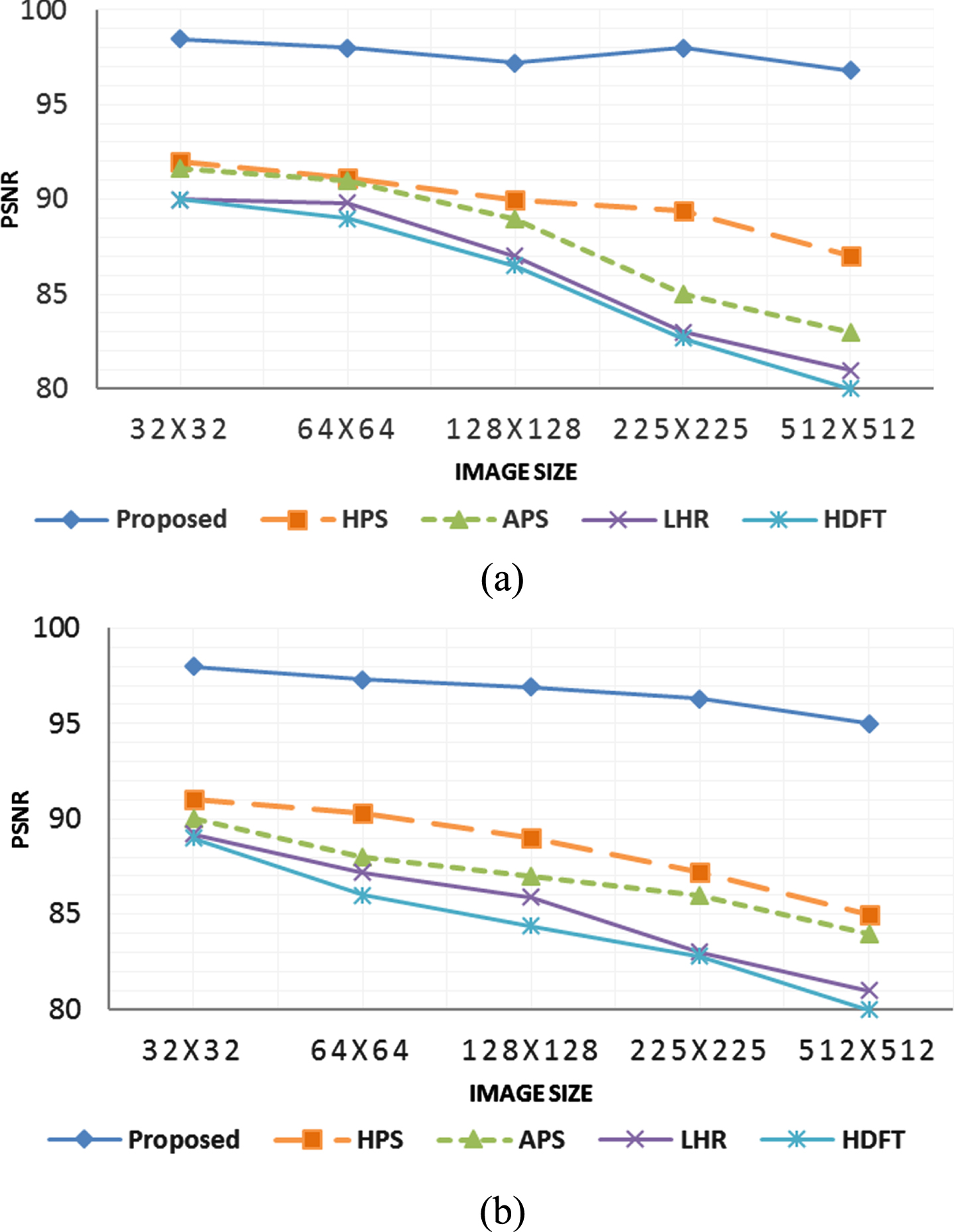
PSNR comparison for various methods under varying image sizes (a) Grey-Scale Image; (b) Color Image.

The rationale behind the PSNR enhancement is the consideration of the equidistant neighbourhood pixels and consistent connectivity from the centre pixel of the proposed method. This consistent connectivity reduces the noise components in the output image which paves a way to yield a noise-free result during the training phase. Furthermore, the pseudo hexagonal pixels in the proposed method produce the output color images with higher pleasant quality. In contrast, the existing methods did not preserve the consistent connectivity that causes undesired artefacts and degrades the image quality.

5.2 Performance analysis of AIC

The AIC of an image has been determined approximately from the simulated images. In general, a higher value of AIC denotes richer information of content and AIC can be calculated by $AIC = - \sum_{n} P_{n} {log}_{2} P_{n}$ (10) where P_n represents the probability where the difference between two neighbouring pixels is equivalent to n.

From Table 3, it is clearly manifest that the proposed 2IHLC method achieves maximum AIC value for both grey-scale and color images. In the case of color image, the proposed 2IHLC method maintains a higher AIC value of 7.62, whereas the HDFT, LHR, APS, and HPS are having 6.40, 6.68, 6.75, and 7.22 AIC respectively. This results owing to attaining an effective hexagonal mesh framework in the proposed 2IHLC method. The effective framework preserves the actual content more efficiently without loss any significant information. Additionally, more than 98%of the pixel contributes to the pseudo hexagonal structure framework simulation that leads to obtaining higher resolution images in the proposed 2IHLC. On the other hand, existing methods exploited complex conversion algorithms to retrieve the original information. They lose many valuable information while processing the high-resolution images.

Table 3

Comparison of AIC results for different methods

Image Size / Methods	Grey-Scale Image					Color Image
	HDFT	LHR	APS	HPS	Proposed	HDFT	LHR	APS	HPS	Proposed
32×32	6.01	6.18	6.22	6.34	6.92	6.12	6.25	6.30	6.98	7.12
64×64	6.20	6.25	6.28	6.42	6.98	6.23	6.37	6.42	7.04	7.27
128×128	6.23	6.30	6.33	6.53	7.03	6.30	6.43	6.57	7.13	7.42
225×225	6.28	6.32	6.30	6.62	7.10	6.35	6.54	6.68	7.20	7.50
512×512	6.30	6.36	6.45	6.67	7.15	6.40	6.68	6.75	7.22	7.62

5.3 Performance analysis of MSE

MSE is generally used to estimate the quality of the image where the higher value of MSE infer that large variation between the input image and hexagonal simulated image. It can be calculated as follows: $MSE = \frac{1}{N} \sum_{i} \sum_{j} {(X_{ij} - V_{ij})}^{2}$ (11) where N is the size of the image, X be the hexagonal processed image, and V denotes the original input image.

It is apparent from Fig. 18 that the proposed 2IHLC outperforms well as compared with existing methods for varying image sizes. The lower value of MSE is obtained by the proposed method because the variation between the input image and the hexagonal simulated image is smaller. Evidently, the proposed 2IHLC method achieves lesser MSE by 46%, 42%, 41%, and 39%as compared to HDFT, LHR, APS, and HPS methods respectively.

Fig. 18

Comparison of MSE for different methods (a) Grey-Scale Image; (b) Color Image.

The key reason behind the smaller MSE is the employment of the simpler operation on the whole image. Besides, the proposed 2IHLC does not require any interpolation filters for image enhancement. This leads to attain lower quantization error and sustain the simulated image with its natural appearance. Alternatively, the Gabor filter is necessitated in the APS and HPS methods for the pre-processing stage. This kind of filters yields more quantization error throughout the image and hence they elucidate a higher MSE value when compared with the proposed 2IHLC method.

5.4 Performance analysis of ART

According to Table 4, it is manifest that the proposed 2IHLC needs a lesser ART than APS and HPS methods. The ART value of the proposed 2IHLC has reduced by 22%, 19%, 14%, and 7%as compared to HDFT, LHR, APS, and HPS methods respectively. In the case of a larger size color image, the proposed 2IHLC method still preserves a minimum ART value of 25.25 ms, whereas the HDFT, LHR, APS, and HPS are having 33.07 ms, 30.98 ms, 29.89 ms, and 27.96 ms ART respectively. This is due to the fact that the proposed 2IHLC method operates with limited conversion parameters during the training phase. As a consequence, it necessitates lesser ART for managing the hexagonal structured image and supports for high-resolution images. This pseudo hexagonal structure maintains clarity in both grey-scale and color images. On the contrary, the existing methods exploit a more number of parameters for simulating the images. They do not evaluate the optimum learning rates for each conversion parameter which requires higher ART and produces a more complex structure.

Table 4
Comparison of ART (msec) results for various methods

Image Size / Methods Grey-Scale Image Color Image

HDFT LHR APS HPS Proposed HDFT LHR APS HPS Proposed

32×32 7.27 6.05 5.15 4.73 4.08 30.12 29.18 27.07 22.41 20.56

64×64 6.93 6.89 6.63 6.11 5.95 31.13 28.17 27.78 23.86 21.87

128×128 7.98 7.77 7.24 6.80 6.30 32.16 29.22 28.05 24.65 22.98

225×225 8.18 8.01 7.93 7.33 6.58 32.69 29.94 28.64 26.53 23.89

512×512 8.34 8.19 8.08 7.45 7.03 33.07 30.98 29.89 27.96 25.25

Image Size / Methods	Grey-Scale Image	Color Image
32×32	7.27	6.05	5.15	4.73	4.08	30.12	29.18	27.07	22.41	20.56
64×64	6.93	6.89	6.63	6.11	5.95	31.13	28.17	27.78	23.86	21.87
128×128	7.98	7.77	7.24	6.80	6.30	32.16	29.22	28.05	24.65	22.98
225×225	8.18	8.01	7.93	7.33	6.58	32.69	29.94	28.64	26.53	23.89
512×512	8.34	8.19	8.08	7.45	7.03	33.07	30.98	29.89	27.96	25.25

5.5 Performance analysis of CEI

CEI is one of the significant quantitative metrics for evaluating the contrast improvement of an input image and it is estimated by $CEI = \frac{C_{i}}{C_{o}}$ (12) where C_i implies the contrast values of the improved image and C_o denotes the contrast values of the original image. On examining the CEI values in Fig. 19, it is proven that the proposed 2IHLC method provides a higher CEI value when compared with existing methods. The CEI value of the proposed 2IHLC has improved by 80%, 74%, 79%, and 62%as compared to HDFT, LHR, APS, and HPS methods respectively. This is because of conserving the contour of each and every hexagonal structure pixel in the proposed 2IHLC method. It also provides a hexagonal simulated images to visually verify without using any hexagonal capture or display device. Higher CEI values expose that the proposed 2IHLC not only recovers the contrast of a simulated image but also enriches the original information in the healthcare image that is more appropriate for the diagnosis process. Conversely, the existing methods do not recover the contrast of a simulated image due to the selection of non-optimum pseudo hexagonal structure. It can be concluded from the aforesaid results that the overall performance of the proposed 2IHLC method outperforms well as compared with existing methods. The proposed method operates more efficiently and robustly in nature while managing various medical images.

Fig. 19

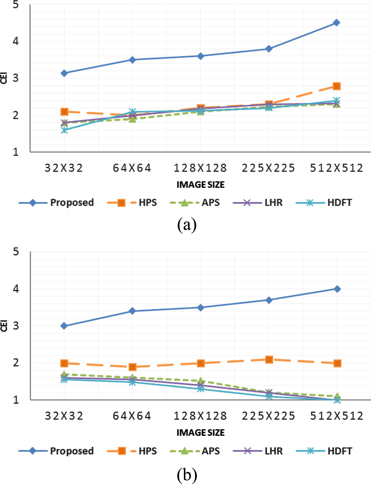
Analysis of CEI for various methods under varying image size (a) Grey-Scale Image; (b) Color Image.

6 Conclusion and future work

In this paper, a new and effective 2IHLC method is implemented in which hexagonal pixels are generated and allow the geometrical symmetry not only to contiguous neighbouring cells but also to the higher-order neighbouring cells. Even though the proposed 2IHLC method is not employing any interpolation filters for image enhancement, the image resolution has been retained and the percentage of unused pixels is very negligible. A highly parallel and real-time simulation is possible in the proposed method owing to consideration of equidistant neighbourhood pixels and consistent connectivity from the centre pixel.

The effectiveness of the proposed 2IHLC algorithm has been evaluated in the Python platform and results clearly manifest that the proposed method outperforms well as compared with existing state-of-the-art methods. In particular, the PSNR value of the proposed 2IHLC has enhanced by 14%, 13%, 11%, and 8%as compared to HDFT, LHR, APS, and HPS methods respectively. This higher PSNR value proves that the proposed method effectively retained the original information from the simulated images. It is capable to produce noise-free images and work accurately even for high-resolution images. Nevertheless, the proposed method has lack of hexagonal imaging and display device. Also, the memory is intensive with high-quality representation of images. In future work, the hex-convolutions will be introduced on hexagonally resampled images. It will also address the different addressing schemes for memory-efficient computations.

References

Choudhury

H.A.

, Sinha

and Saikia

, Application of nature-inspired algorithms (NIA) for optimization of video compression, Journal of Intelligent & Fuzzy Systems 38(3) (2020), 3419–3443.

Karkishchenko

and Mnukhin

, Hexagonal images processing over finite eisenstein fields, Procedia Eng 201 (2017), 287–295.

Wang

, Ni

and Guo

, Modulation transfer function of an imaging system with a hexagonal pixel array detector, Optik 179 (2019), 986–993.

Jing

, Coleman

, Scotney

, Biologically motivated spiral architecture for fast video processing, 2015 IEEE International Conference on Image Processing (ICIP). IEEE, (2015), 1–7.

Neubert

, Schubert

and Protzel

, An introduction to hyperdimensional computing for robotics, KI-Künstliche Intelligenz 33(4) (2019), 319–330.

Ribeiro

, Cardoso

, Bernardino

, Highly sensitive bio-inspired sensor for fine surface exploration and characterization, IEEE International Conference on Robotics and Automation (ICRA). IEEE (2020), 1–8.

Byanju

, Arne

, Hansen

and Akram

M.N.

, A comparative study of superimposition techniques for enhancing the projector resolution: Simulations and experiments, Displays 55 (2018), 80–89.

, Xiao

, Wang

and Qi

, A brain–computer interface based on miniature-event-related potentials induced by very small lateral visual stimuli, IEEE Transactions on Biomedical Engineering 65 (2018), 1166–1175.

Kalli

, Suresh

, Prasanth

and Muthumanickam

, An effective motion object detection using adaptive background modeling mechanism in video surveillance system, Journal of Intelligent & Fuzzy Systems 41 (2021), 1777–1789.

10.

Wang

, Zhong

and Zhang

, Spatial group sparsity regularized nonnegative matrix factorization for hyperspectral unmixing, IEEE Transactions on Geoscience and Remote Sensing 55 (2017), 6287–6304.

11.

Luo

, Zhang

and Su

, Hexagonal Convolutional Neural Networks for Hexagonal Grids, IEEE Access 7 (2019), 142738–142749.

12.

Coleman

, Scotney

and Gardiner

, Tri-directional gradient operators for hexagonal image processing, Journal of Visual Communication and Image Representation 38 (2016), 614–626.

13.

, Implementation of a simulated display for hexagonal image processing, Displays 50 (2017), 63–69.

14.

Gardiner

, Coleman

S.A.

and Scotney

B.W.

, Multiscale edge detection using a finite element framework for hexagonal Pixel-based images, IEEE Transactions on Image Processing 25 (2016), 1849–1861.

15.

Luczak

Ed.

, Rosenfeld

, Distance on a hexagonal grid, IEEE Transactions on Computers, C-25 (1976), 532–533.

16.

Ahir

and Satyanarayana

R.V.S.

, Three-Dimensional Image Compression Using 2.5 D Spatial Subsampling and Reconstruction Using 2.5 D Morphological Filters, IUP Journal of Telecommunications 11 (2019), 22–35.

17.

Mersereau

R.M.

, The processing of hexagonally sampled two-dimensional signals, Proceedings of the IEEE (1979), 930–949.

18.

Jeevan

K.M.

and Krishnakumar

, An algorithm for the simulation of pseudo hexagonal image structure using MATLAB, International Journal of Image, Graphics and Signal Processing 57 (2016), 57–63.

19.

Fadaei

and Rashno

, A Framework for Hexagonal Image Processing Using Hexagonal Pixel-Perfect Approximations in Subpixel Resolution, IEEE Transactions on Image Processing 30 (2021), 4555–4570.

20.

Petersen Daniel

and Middleton

, Sampling and reconstruction of wave-number-limited functions in N-dimensional Euclidean spaces, Information and Control 5 (1962), 279–323.

21.

Kamgar-Parsi, Behzad , Sander

W.A.

, Quantization error in spatial sampling: comparison between square and hexagonal pixels, Proceedings CVPR’89: IEEE Computer Society Conference on Computer Vision and Pattern Recognition. IEEE, (1989), 1–10.

22.

Parsi Behrooz

and Kamgar-Parsi

, Evaluation of quantization error in computer vision, IEEE Transactions on Pattern Analysis and Machine Intelligence 11(9) (1989), 929–940.

23.

Richard

, Rafael

, Digital Image Processing, 2nd Edition, Addison-Wesley, November (2001).

24.

Mylopoulos John

and Pavlidis

, On the topological properties of quantized spaces, I. the notion of dimension, Journal of the ACM 18 (1971), 239–246.

25.

Golay, Marcel

, Hexagonal parallel pattern transformations, IEEE Transactions on computers 18(8) (1969), 733–740.

26.

Sonya Coleman

, Bryan Scotney

, Bryan Gardiner , Design of Feature Extraction Operators for Use on Biologically Motivated Hexagonal Image Structures, MVA (2009),1–7.

27.

Serra

, Introduction to mathematical morphology, Computer vision, graphics, and image processing (1986), 283–305.s

28.

Cuevas

, Rodríguez

and Alejo-Reyes

, Clustering Model Based on the Human Visual System, Recent Meta-heuristic Computation Schemes in Engineering. Springer 948 (2021), 169–192.