
Abstract
This paper deals with the design and development of a novel approach, centered on the creation and development of a fuzzy controller to analyze electroencephalogram (EEG) data. The fuzzy controller makes use of the functions associated with the different regions of the brain to correlate multiple Brodmann areas to several outputs, where a normal analysis would associate only one region to one output. This controller was designed to quickly adapt to any data imported into it. The current implemented framework supports a math study. The math subjects’ outputs were attuned to their related study which involved transcranial direct current stimulation (tDCS), which is a form of neurostimulation. Anode affinity, cathode affinity, calculation, memory, and decision making were the outputs focused on for the math study. This task is best suited to a fuzzy controller since interactions between Brodmann areas can be analyzed and the contributions of each area accounted for by indicating which regions have stronger and weaker effects on any given output.
Keywords
Introduction
Problem background
Electroencephalography (EEG) is a tool used to better understand the inner working of the human brain. By utilizing the bioelectrical potentials generated by the cortex nerve cells within the brain, it is possible to identify which areas of the brain are active [1]. EEG can be either invasive or non-invasive based on the equipment used, but it is more commonly non-invasive with the advancements made since its invention. EEG is an important part of understanding neurological disorders, such as, epilepsy, brain tumors, and locating head damages [2, 3]. Transcranial direct current stimulation (tDCS) is a form of neurostimulation that has been researched, in recent years, as a means of treating cognitive deficiencies. tDCS is a noninvasive stimulation for the brain. By using a pair of electrodes, it is possible to excite the cerebral cortex. The range of applications is vast, ranging from medical issues to learning and training [4]. In the medical field, tDCS has been applied to different neuropsychiatric diseases and disorders including depression, epilepsy, electroanalgesia, stroke, schizophrenia, and Parkinson’s disease [4]. tDCS can also be used to enhance performance during cognitive tasks. There have been studies that report tDCS can facilitate training-related performance improvements during simple motor tasks as well as enhancements in the planning abilities of subjects [5, 6]. Cosmo (2015) found that there was an increase in cortical connectivity after stimulation of the left dorsolateral prefrontal cortex (DLPFC) in sixty attention-deficit/hyperactivity disorder (ADHD) patients. His results suggested that the effects of tDCS are selective based upon the patient. The contributors to variability within individuals include genetics, gender, age, hormone level, and time of day. In tDCS, parameters such as electrode size, current intensity, and current density also affect stimulation, which can lead to an even greater variability between studies [7].
Problem description
Electroencephalography (EEG) measures the bioelectrical signals within the brain. This is done with the aid of an EEG cap that holds the electrodes in place. The cap electrodes then measure the bioelectrical potential relative to a determined ground electrode. These potentials are generated by the cortex nerve cells within the brain [1]. This allows for the collection of brain activity from the surface of the scalp. In this way, it is not necessary to use any invasive methods, as EEG data collection can be done by contacting the surface of the scalp. Unlike magnetic resonance imaging (MRI), EEG can only collect the electrical signals on the surface of the scalp. In order to find the sources of the EEG signals, Standardized Low Resolution Brain Electromagnetic Tomography (sLORETA) can be used to calculate the origin of the signals within the brain. LORETA provides a 3-D model of the brain with the excitation and area of excitation detailed at any given point and time desired [2]. The data is recorded and sent back into MATLAB to finish the final section of the problem. The final interpretation of the data is subject to a level of uncertainty. Due to this, it is a perfect application for an artificial intelligence fuzzy logic controller as this would allow for data to be processed with membership values. With this fluidity in the data analysis, it is possible to complete parts of the analysis before explicitly categorizing certain aspects of the data. Then, the output of the controller can be used to better understand the data, the process of tDCS, and how to improve future sessions. Fuzzy sets’ ability to handle ambiguity allows a more streamline approach to analyze data gathered from sLORETA. During the analysis of the generators in the brain, there is a spread of multiple regions used throughout the session. Fuzzy set theory can be used to analyze the frequency and the likelihood of each region being related to the task at hand. This can identify the most used region, as well as other related area of the brain related to the task in question.
With these regions mapped out, tDCS can be used to better target the generators employed for the task. Fuzzy logic can then be useful to determine which areas to target and which configuration best fits each individual going through tDCS stimulation. A fuzzy set controller can thus be designed to take in multiple conditions to be considered, including seemingly abstract details, which could account for initially unseen connections between variables and outputs.
Research scope and objectives
With tDCS gaining more popularity in recent years, it is important to understand how exactly it affects the subject’s brain. Tools like EEG, TMS, and MRI have been used through the years. Each has its advantages and disadvantages, as discussed earlier. By using EEG, one can observe the activity on the surface of the scalp, but not where that activity comes from within the brain. With MRI, it is possible to observe the inner workings of the brain, but the technology limits movement and most machines require one to be stationary inside a tube. The solution to these problems involves developing a series of models that show where the generators in the brain activate on the scalp. This is the forward solution, i.e. taking into account how the activity flows normally. Through data from multiple studies, Standardized Low Resolution Brain Electromagnetic Tomography (sLORETA) can be used to solve the inverse problem. With the source localization built into sLORETA, the activity on the surface of the scalp allows sLORETA to determine where the activity within the brain originated [15].
Literature review
tDCS is accomplished by polarizing the human brain’s resting membrane potential. If administered for several minutes, the excitability can outlast the time stimulated, allowing tDCS to be used for neurological and psychiatric disorders. Early studies by Nitsche and Paulus (2000) showed that the effects produced by applying tDCS at 1 mA for 10 minutes while using 35 cm2 electrodes could last up to one hour after stimulation [3]. It was also shown that higher current intensities produced greater changes to the cortical excitability, between 1 mA and 0.2 mA. Since then, 35 cm2 electrodes have been in common use. This suggests that a higher current produces a greater and longer lasting effect, but it is uncertain if the current density, and not the intensity, is causing these lasting effects [4, 6].
tDCS administration
For most studies, the main parameters are current intensity (mA), electrode size (cm2), electrode placement, and duration. Current density (mA/cm2) is calculated from dividing the current intensity over the electrode area. Most studies follow the findings of Nitsche and Paulus (2000) about polar specific tDCS where the anode excites, and the cathode inhibits. It is also suggested that higher current intensities and longer stimulation produces stronger and more lasting effects. This was later challenged by further studies that showed that there is a nonlinear relationship between current intensity and stimulation, and further by the lack of difference in efficacy between two or three different current intensities of anodal tDCS [5]. Ho and colleagues (2015) researched the impact of current intensity (mA) and electrode size (cm2) on motor cortical excitability. These are factors that relate to current density (mA/cm2), which is considered an important factor in the outcome of tDCS. By manipulating these key parameters, the outcome of the stimulation can be altered [4].
Standard parameters for administration of tDCS
tDCS administrating parameters can be changed, but usually they are kept within certain bounds. Current intensity usually ranges from 0.2 mA to 2 mA, for safety reasons. It was also suggested by Ho et al. (2016) that the following are the significant parameter relationships: “1) size of the electrode relative to the size of the target, 2) location of the electric field relative to the target area and 3) direction of the electric field relative to the neuronal orientation” [4].
The size and shape of the electrodes compared to the area of stimulation matters. Tailored electrodes are thought to result in a greater increase in excitability when compared to standard non-tailored electrodes [4]. When an electrode is larger than the target area, it may not effectively stimulate the underlying cortex as the current distribution becomes diffused to the point where it is functionally inert. In common practice, electrodes are placed centered over the hotspot, but computational modeling suggests that the peak current densities are actually in-between the electrodes, closer to the anode. The motor hotspot likely still receives some stimulation, but the peak current densities may be peripheral to the hotspot. The electric field also has a direction, as it travels through the brain, which interacts with the neuronal orientation. The standard montage involves the anode on the motor cortex with the cathode on the contralateral supraorbital area to produce excitability, while the opposite orientation produces no excitability. The mechanisms underlying tDCS and its effects are likely multifactorial, and therefore, it is important to consider all the factors involved. If any factor is suboptimal, such as current direction, the excitability could be reduced or negated all together [4].
Long- and short-term effects of tDCS
tDCS has been performed in hundreds of reported studies to date, all of which have not seen any serious side effects, in healthy controls and patient populations [6, 7]. The extent of side effects is limited to slight itching under the electrode, headache, fatigue, and nausea. Side effects are usually limited to a minority of cases of more than 550 subjects [7, 8]. These studies have shown the safety of tDCS. In patients with skin diseases, it is possible that non-intact skin will experience tissue heating. tDCS has shown no evidence of toxic effects to date over the thousands of subjects worldwide. There have been numerous studies explicitly focused on safety [7–9]. Poreisz et al. (2007) reviewed the adverse effects of 77 healthy subjects and 25 patients over the course of 567 1-mA stimulations [8]. The side effects experienced were broken down by the following percentages: 75% mild tingling sensations, 30% light itching sensation, 35% moderate fatigue, and 11.8% headache. Most of these did not differ from the placebo stimulation. The most severe side effect reported was skin lesions on the site of the electrode [9].
Efficiency of tDCS and potential complications
An optimal set of parameters is not defined for tDCS. It is unclear whether alteration of treatment parameters such as session frequency, number of sessions, or current intensity enhances the efficacy of tDCS. Alonzo et al. (2012) found that over a five-day period, subjects who received tDCS daily, as opposed to twice daily, had greater neuronal excitability. It is important to note that the amount of sessions received and not the frequency of sessions may have favored the results of the daily tDCS [10]. To measure the effects of tDCS, a few methods can be used. The excitability can be measured in the motor cortex using transcranial magnetic stimulation (TMS). Electromyography (EMG) can be used to record the motor evoked potentials (MEPs) [4].
tDCS efficiency and efficacy
Clark et al. (2012) were able to apply tDCS to reduce the time required for subjects to learn a skill [11]. From their fMRI studies, it was determined that the right inferior frontal (RINF/RIF) and right parietal cortex (RPAR), as well as the temporal, cingulate and other brain regions, make up the parts of the brain involved with concealed threat-related objects in the naturalistic environments. Eighty-three healthy subjects participated in varying levels of tDCS at different scalp locations. The second form utilizes fMRI to measure the blood oxygen level dependent (BOLD). The BOLD responds were compared for the scenes with concealed threats and those without. FMRI values were collected as the participants started as novice and proceeded through intermediate then to expert. Readings were also collected an hour after stimulation. These results are relative to the individual’s baseline and were taken immediately after training. As stated earlier, Alonzo et al. (2012) found that over a five day period, subjects who received tDCS daily, as opposed to twice daily, had greater neuronal excitability [10]. By using surface electromyography (EMG), it was possible to measure the motor evoked potentials (MEPs) from the first dorsal interosseus (FDI). The readings were taken with respect to the baseline measured during the trials.
Methods of software analysis for tDCS
With tDCS becoming more popular, further in-depth analysis of what happens in the brain during stimulation is needed. Computational simulations allow the independent determination of the most likely patterns of current flow and current density during tDCS. Sadleir et al. (2010) used a finite element model to depict several individuals. Models of entire heads were created which included data for the conductivity of bone, scalp, blood, CSF, muscle, white matter, grey matter, sclera, fat, and cartilage. Sadleir et al. (2010) observed current densities beneath the electrodes were large in tissues such as skin, muscle, and CSF. In lower conductivity areas, such as fat and bone, the current densities were lower even near the electrodes [12]. In 2009, Hyun Sang used 3-D high resolution finite element analysis (FEA) to gain a precise analysis of the electromagnetic effect of tDCS [13]. A realistic head model was developed with anisotropy of the white matter and the skull. Their results show that the skull anisotropy, tissue anisotropy, and white matter affect current flow. The skull anisotropy induces a strong shunting effect, which causes a shift in the stimulated area. The white matter strongly affects the current flow, which changes the current field distribution inside the brain. Tissue anisotropy significantly affects how the brain is stimulated in its deeper areas. It is also important to note that the brain is made up of three sub-regions, each with its own conductivity. These sections include one soft bone layer which is surrounded by two hard bone layers. Only one compartment was used in this study [13].
Chang-Hwan Im et. al (2009) also modeled the conductivity and the electric field of a head using 3 D finite element method (FEM). By using the structural metrics from MRI data, a finite element model was extracted. The scalp surface was roughly approximated as a sphere, allowing the use of spherical coordinates. By optimizing the angles and locations of the electrodes based on the data, Chang-Hwan was able to create a model showing optimized electrode locations for a given target area deep in the brain [14].
Significance of this research work
As shown by the available published literature, there has been a recent increase in tDCS research. Its vast range of potential uses allows tDCS to be used for medical applications as well as task-oriented situations. While many studies have shown the benefits of tDCS, there are very few reported studies that explore how the initial generating neurons are affected. By utilizing EEG data, and solving the inverse problem, it is possible to determine where the surface data originated from. This would show if the areas targeted by tDCS stimulation were indeed stimulated, as intended. A postulate here is that through fuzzy sets, it is conceivable to analyze multiple subjects and discern if tDCS was applied, as well as where the maximum stimulation occurred for each subject. Moreover, other key factors can be determined as well, such as how long the stimulation lasted and how much it changed over time. In this way, a better understanding of control and tDCS subjects can be developed. This research work focused on using that understanding to aid in tDCS administration. By doing so, tDCS can better enhance the brain regions determined to be most utilized during the task at hand. Since the methodology is set up specific rules to analyze the data and determine conclusions, it can be applied to any task.
Materials and methods
Field data
The conducted study used tDCS data from a previous research investigation carried out between 2015 and 2017 that involved collecting EEG data via mobile and stationary amplifiers in a pilot study focused on the impact of low current brain stimulation on math understanding and calculations. Data was collected using a 64-channel mobile EEG amplifier from tDCS subjects. During the study, undergraduate math students were monitored. They were divided into two groups of individuals, one of which was the control group and the other the experimental group. All the participants consisted of freshman and sophomore engineering students at The University of Alabama. The students were enrolling in a pre-calculus algebra course (i.e. Math 112). Phase one included a baseline assessment of the study group, in which basic EEG data was taken, without tDCS. After the baseline recording were taken, a video discussing intermediate algebra calculations was shown, while still taking EEG data. Two baseline assessments were made with different videos.
Low current brain stimulation was administered to the experimental group, with the anode (positive electrode) placed on P3, based on the 10–20 international system of EEG electrode placement shown in Fig. 1. This is due to P3 being associated with calculations and reasoning. The cathode (negative electrode) was place at T4 based on the 10–20 international system. The experimental group was administered 2 mA over 20 minutes for each instance. The control group was given a sham condition in which the administration provided was 1.0 mA, lasting for 30 seconds. To replicate the same experience, the control subjects were treated as though they were given tDCs for the full 20 minutes. After watching the algebra video, subjects completed calculations based on instructions received from the video. Data collection was gathered from 64 electrode sites e.g. Fp1, Fp2, F7, F3, Pz, F4, F8, T3, C3, Cz, C4, T4, T5, P3, Pz, P4, T6 O1 & O2. The maximum sampling rate was 2048 Hz.

10–20 international electrode placement [16].
Test data was processed through a data acquisition program called asalab. The built-in tools of asalab allowed for an effective filtering of the acquired data. After the filtering was done, the data needed to be converted into a format that LORETA can read in order to calculate the source localization to determine where the initial neuron that generated the surface excitation was located. By using the EEGLAB interactive MATLAB toolbox developed by Swartz Center for Computational Neuroscience, it was possible to convert the data taken with asalab to LORETA.
Figure 2 shows unfiltered data represented in EEGLAB. These high spikes, which are noise in the data, will be accounted for during the filtering process.
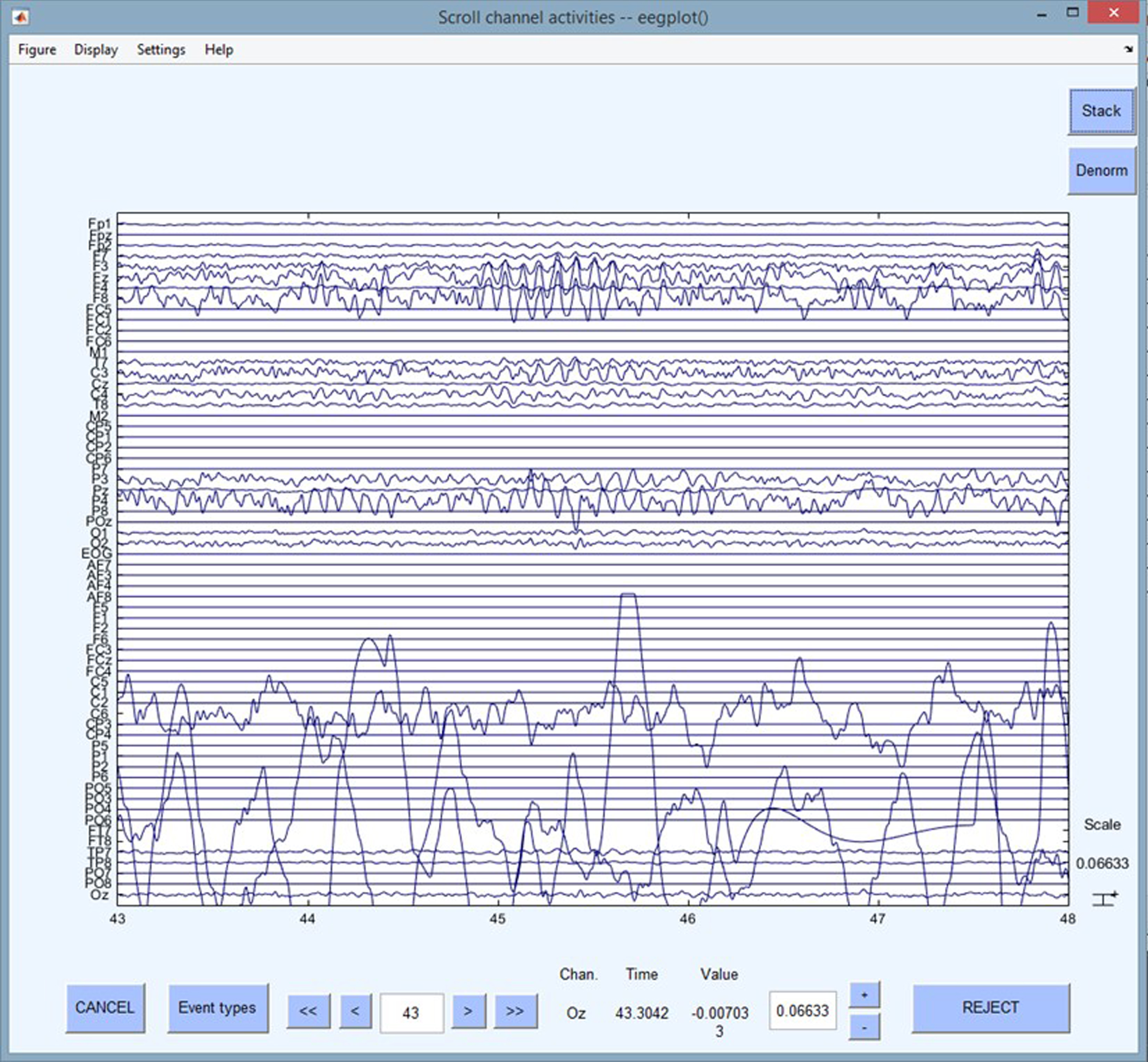
Unfiltered data represented in EEGLAB.
In order to streamline the filtering process, a MATLAB script was written. The first section of the script allows for multiple subjects and sessions to be loaded at once from a file location on the computer. The script first looks into the folder detailed in the script. It then makes a list of every type of file of the specified type. In this case, set files were taken. The script proceeds to iterate through each file until every file has been processed.
The processing of the data starts with loading the data from the list of files. Once loaded, the unused channels are removed and only the specified channels requested in the script will remain. At this point, the script loads the standard locations of the remaining channels to be later used for interpolation purposes. The script runs ICA, followed by a purge of any bad channel components. This is when the channel locations from earlier allows for interpolating back any rejected data using the location of the channels nearby. The script then sections the data off into segments based on length or parameters defined in the script. These segments are subsequently filtered before they are standardized in length to be loaded into LORETA.
Before the collected data could be used, certain parameters, such as the electrode configuration, needed to be established within LORETA. When input into LORETA, the electrodes were still in the 10–20 international system, but sLORETA uses Talairach coordinates, which corresponded to where the electrodes are on the scalp spatially. It is possible to measure these spatial coordinates per individual, but LORETA has built in models that were averaged over many participants to compute mean coordinates relative to each channel location. LORETA then took these coordinates and calculated a transformation matrix for sLORETA or eLORETA with a chosen regularization method. The EEG files could then be processed with sLORETA using the transformation matrix. This produced viewing files that can be observed over any given time frame.
Time frames were chosen based on the checkpoints determined to better understand what occurred during the study. Based on its overall time, the session was broken up into five sections and analyzed with sLORETA. The start window showed how the brain is adapted to tDCS and the task conducted. The next section of the data made it possible to examine how the brain adapted to the task. During the third section of the data, the brain was well enthralled in the task at hand. The fourth section was used to observe how well the brain maintained focus. Finally, data from the last section was used to determine how the brain reacted as the activity is finishing, and how well the stimulation lasted. Example data from sLORETA is shown in Fig. 3.

Data from sLORETA data showing cross sections of brain activation.
Based upon the collected data, as well as correlations from the available literature, it was possible to develop a set of fuzzy inputs and outputs. Fuzzifying the results was based on the region of the brain being active, and level of activation. The rules that defined the controller were developed based on the data and programmed with MATLAB’s Fuzzy Toolbox through a Mamdani controller scheme, a centroid based method. The resulting controller was then tested at known states to compare desired stimulation and the resulting output parameters.
The fuzzy controller was used to analyze the data by correlating the levels of activation of every participant at each given time. This fuzzy controller determined trends in the data. Once trained, the controller was able to establish whether or not tDCS had an impact on the brain. It also assessed the level of activation to expect in future studies, as well as which regions were most activated during the task, along with any secondary regions that showed to share/hinder the activation of the main region of the brain. The controller was constructed in an input/output user friendly fashion. There is also the potential to incorporate additional rules, inputs, and outputs to the controller, as needed. A flowchart depicting the in-depth methodology followed in this research study is shown in Fig. 4.

Research Project Flowchart.
EEG data was recorded using asalab, and simple noise filters were applied. The data was then exported for use in EEGLAB. At this point, a better understanding of EEGLAB was necessary to filter the data and prepare it for sLORETA. The data was then exported in a form that sLORETA could read and use.
Initially, one set of data was filtered and analyzed to determine key parameters to analyze the data e.g. filtering thresholds, segment lengths, Brodmann areas and activation. These parameters were later used to process and analyze the remaining data sets. Data from this analysis were used to generate inputs and outputs for the fuzzy controller. The rules for the input and outputs were setup to establish the functionality of the controller as it takes and processes data. Developing a fuzzy controller prototype furthered the understanding of how the EEG data should be filtered and analyzed. Afterwards, the remaining data points were filtered and processed with sLORETA.
The fuzzy controller was developed to identify trends in the activity over time, location, and duration. The controller was tuned to increase its accuracy in determining these trends. It was then enhanced to assess how best to improve stimulation on the grounds of how well each subject matched up to the rest of the study group. In the case of single individual trials, there is no comparison group, so the controller was based on the individual’s previous stimulation trials. The accuracy of the controller was critiqued further with discussion from domain experts in tDCS administration at the University of Alabama. Lastly, the controller’s heuristics were fine-tuned to account for additional variables.
Determining inputs
An initial analysis of the data was done to see which Brodmann areas had the highest excitation among all the candidates during the sessions. The Brodmann areas are the sections of the human brain responsible for controlling the receptors throughout the body that recollect sensations associated with touch, pain, temperature, and localization of touch. This region is also important for skilled and coordinated movements as well as motor learning. The areas of interest and excitation in voxels were Brodmann areas 7, 9, 10, 11, 20, 21, 39, and 47. Their locations can be seen in Fig. 5. Due to the nature of Brodmann areas, there are multiple stimuli that excite any given area. For this reason, the following descriptions of the Brodmann areas focus on the generalized role along with any relevant notes. A broader explanation of each area can be found in the Cortical Functions Reference Manual (2012). Areas will be presented in numerical order starting with Brodmann area 7 [17]. Brodmann area 7 is referred to as the somatosensory association cortex. It is part of the parietal cortex, which is believed to play a role in visuo-motor coordination, such as reaching to grasp an object. The region that Brodmann area 7 (the superior parietal lobe) is associated with rhyme detection and semantic categorization tasks, along with temporal context recognition. Some additional processes worth noting are association with working memory (motor, visual, auditory, emotional, verbal) [17].
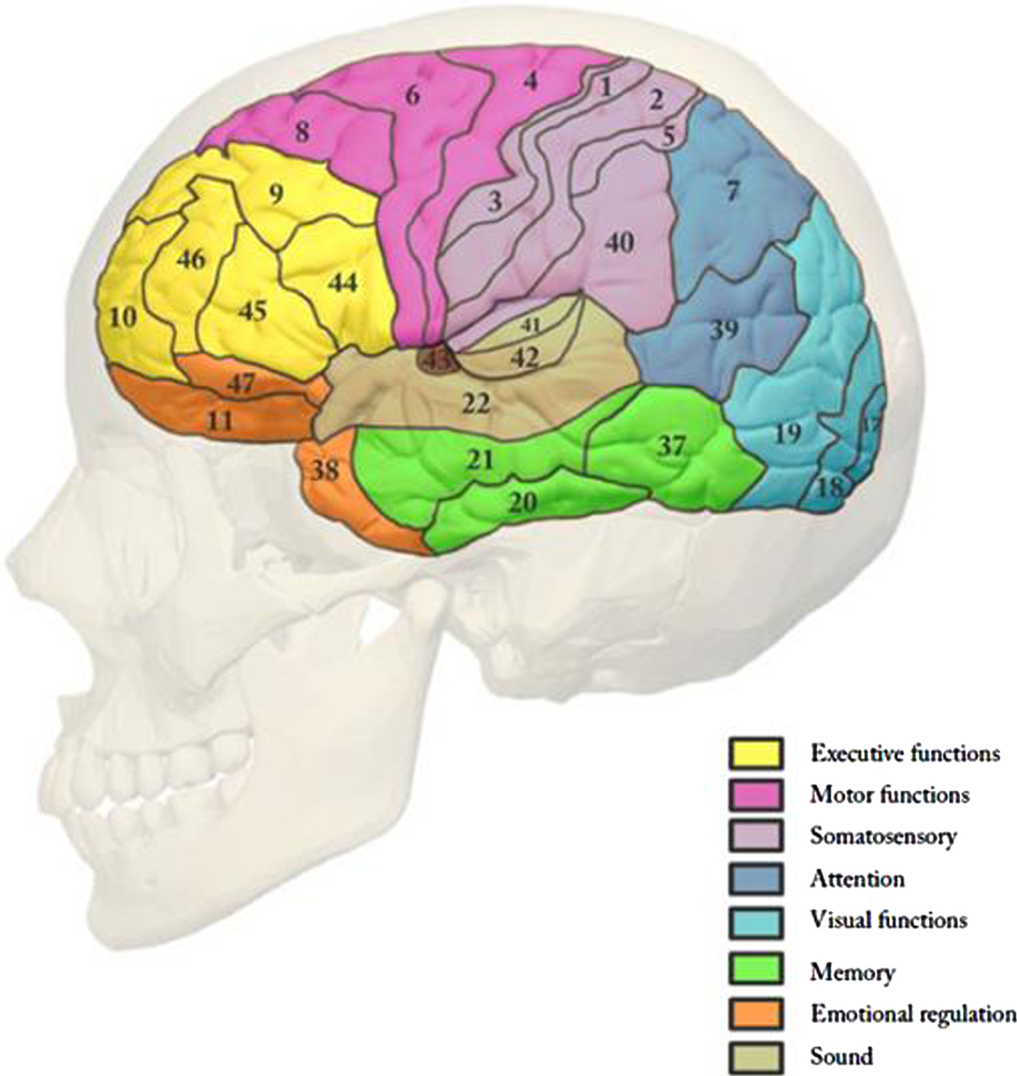
Brodmann Cortical Areas [17].
The dorsolateral prefrontal cortex includes Brodmann areas 9 and 46, by a more restricted definition, but in a broader definition, it also includes areas 9 through 12 along with 45 through 47. Areas 9 and 10 are significate in brain operations involving memory. More specifically, in memory encoding, memory retrieval, and working memory. Brodmann areas 9 and 10 show certain executive functions as well. These include “executive control of behavior”, “inferential reasoning”, and “decision making”. There is a long list of additional processes, but the ones of note to this study include: Error processing/detection, attention to human voices, and calculation/numerical processes [17].
Area 11, the orbitofrontal area, is associated with general olfaction, nonspeech processing, decision making involving reward, and face name association. This area covers the medial part of the ventral surface in the frontal lobe, meaning that it is near areas 9, 10, and 47 [17].
The inferior temporal gyrus is area 20, which is part of the temporal cortex. This area is believed to be a major part of high-level visual processing and recognition memory. Also, worth noting is visual fixation and dual working memory task processing. Area 21 is the middle temporal Gyrus. Its exact function is unclear, but holds connections to processing distance, recognition of known faces, deductive reasoning and accessing word meaning while reading [17].
Area 39 is the angular gyrus. This area is associated with a number of processes including language, mathematics and cognition, including theory of mind. The left side in particular involves calculations, arithmetic learning, and abstract coding of numerical magnitude [17].
Lastly, the inferior prefrontal gyrus is area 47. Area 47 is involved in many functions related to language and emotion. Other processes include working memory, nonspatial auditory processing, decision making, and deductive reasoning [17].
A fuzzy controller based on the Mamdani control algorithm was developed to identify trends in the activity over time, location, and duration. The unique part of a Mamdani controller is its rule base. It works by determining the input’s degree of membership in the rule-antecedent, computing the rule consequences, and then totaling the rule consequences to determine the fuzzy set “control action". The degree of membership is based upon the chosen operator. Following this, the rule consequences can be determined by clipping the consequence to the maximum value of such a membership. The final output of the control is then de-fuzzified and utilized as an input in a feedback loop.
The controller was tuned to increase its accuracy in determining these trends. It was then enhanced to assess how best to improve stimulation on the grounds of how well each subject matched up to the rest of the study group. In the case of single individual trials, there is no comparison group, so the controller was based on the individual’s previous stimulation trials. The data was organized into columns based on Brodmann Area and the rows were based on time. In the controller creator script, there is clear distinction between the required inputs that need to be changed and then the rest of the script that can be changed, as desired, to add additional functionality. The script is commented to allow for easier visualization and aids the user in finding areas to add unique nuances for their data set. The most impactful section for the output of the controller is the rule generation. This is where the most thought and time was focused. Figure 6 shows the process of rule generation for the math study. The Brodmann areas are first associated with the Brodmann cortical regions shown in the blue column. The rule column provides a more detailed explanation of each input. These descriptions are then mapped to the chosen outputs based on their perceived effect on each output. The green, blue, and yellow lines represent high, medium, and low effect, respectively [17].

Rule generation for the math study.
The order of rules determines how the rules appear in the rule viewer. Figure 7 illustrates the appearance of the rule viewer. It is a visual representation of each individual rule. The inputs can be changed to observe how the outputs react. This can be used to understand how each rule affects the output. The input at the bottom left of the rule viewer can be changed to subject data to see the breakdown for each subject.

MATLAB rule viewer showing the breakdown of outputs based on rules.
The process of creating rules in the script is shown in Fig. 7. The script requires a specific syntax for the rules. The “==” sign is used for variables to show that particular variable is equal to high, med, or low. “BA39==High =>Calculations=High” means that when Brodmann area 39 is high then this output calculations is high. There is also coding for “or” and “and” shown by | for or and & for and. In addition, the “∼=” sign can be used to show that the output is true when the input is not equal to low. “BA39∼=High & BA20==High=>Cathode Affinity = High” means that when Brodmann 39 is not low and Brodmann area 20 is high then there is a high Cathode Affinity. The rule variable is setup with the first rule, being the rule(1)=. The rest of the rules should follow the same format of rule(end +1)= which adds the current rule to the end of the rule matrix, which ultimately is merged into the controller. At the bottom of the rule viewer, the culmination of the rules and the defuzzification method are indicated by the red lines on the right-hand side (Fig. 7).
This study focused on tDCS data; thus, the outputs include anode affinity, cathode affinity, calculations, decision, and memory. The full outputs are shown in a heat map displayed in Fig. 8. To offset the fact that defuzzification with the centroid method never gives a score of 100, the data has been normalized. The script was run, and data analyzed incrementally which allowed the rules to be evaluated and tuned each iteration for more accurate results. The script also displays z-scores based on local and global data as shown in Figs. 9 and 10, respectively. Each subject has a C or an E after their subject number, such as 1 C and 3 E. The C stands for “control” and E for “experiment”. The E subjects are the tDCS stimulated individuals.
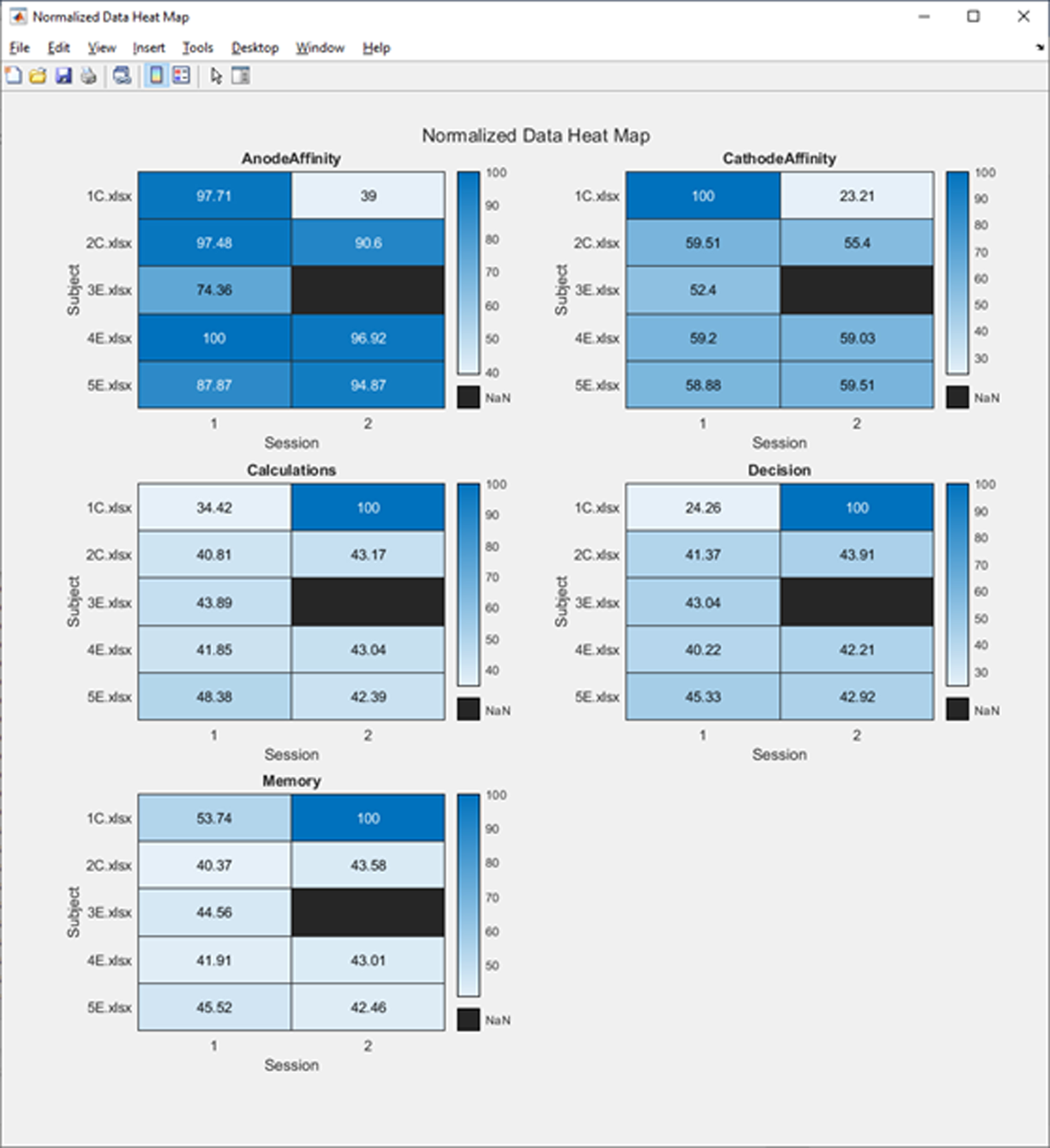
Math study normalized data.

Math local z-score heat map.
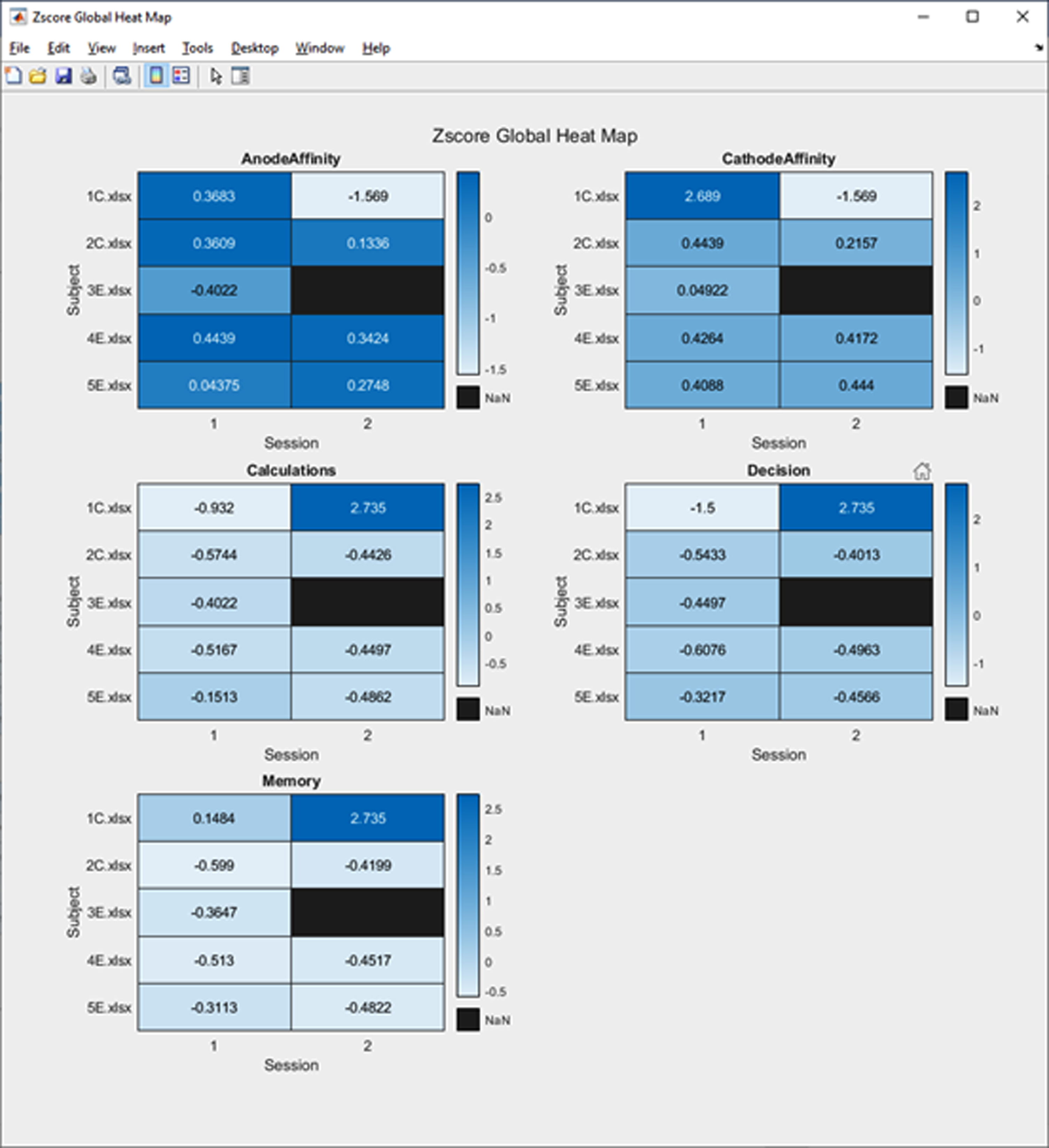
Math global z-score heat map.
An additional analysis (Fig. 11) interprets the out-puts as data points in a 5th dimensional space. This allows for the distance formula to be utilized to determine how different (far away) or similar (close) the datapoints are. The heatmap is used to show the distance from one session to the next. The darker colors represent data that is further apart, and the lighter colors represent data that shares a similar area in 5th dimensional space, representing sameness in the datapoints.
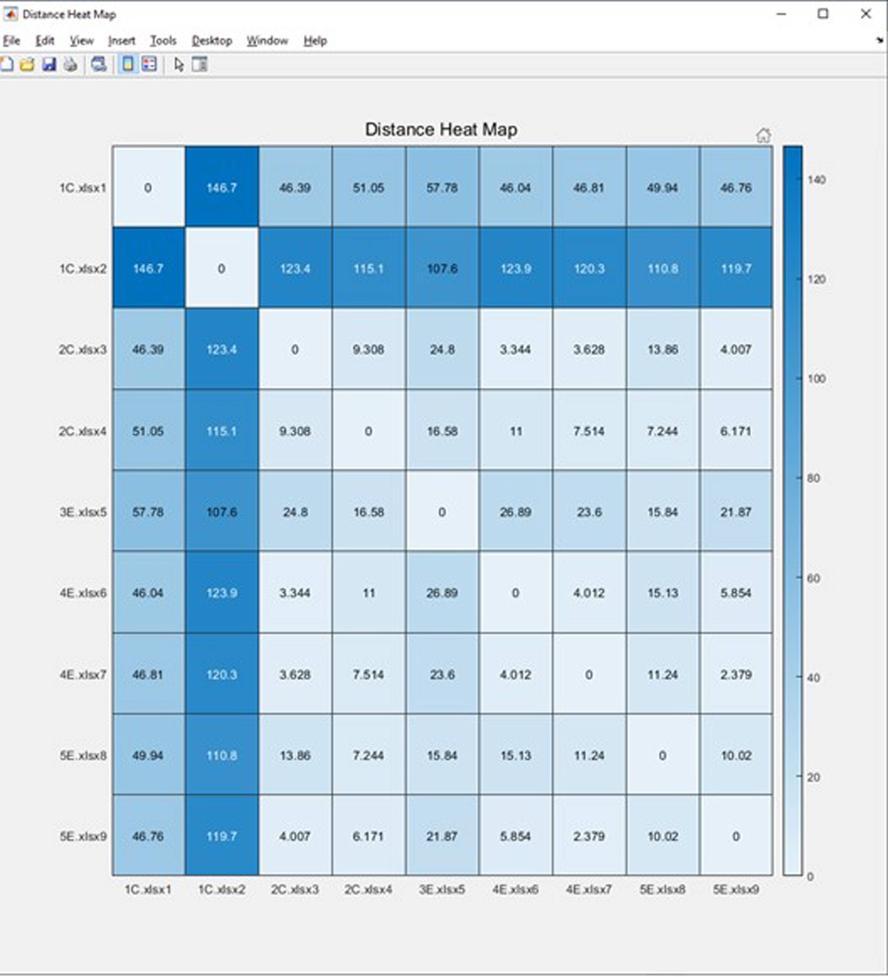
Math Distance Heat Map.
Since this study involved the analysis of tDCS data, the point of interest is on how that stimulation affected the activation of the brain. For a stream-lined discussion and responses, rankings of the out-puts are shown in Fig. 12. The numbers in the chart indicate calculations means that among all of the five outputs, calculations was the lowest. Conversely, a one indicates that this output was the highest, and therefore, the most activated area during the session.

Ranking of Math Study Data.
In Table 1, Subject 1 C was excluded in the heatmap made automatically with MATLAB as this subject was skewing the data. Subject 1C’s rankings are displayed in Table 1, along with the other subjects. Subject 1 C was a control subject and therefore did not receive an application of tDCS. In session one, Subject 1 C showed the most activation in the cathode region of the brain. While the subject did not receive any stimulation, this still indicates it was a region of interest in this particular session. As for the rest of the subject’s outputs, memory and calculations over decision making were favored. This indicates that Subject 1 C focused on remembering the skills taught and applying them. The need for decision making was lower due to the level of consideration in determining the final answer of the given math problem or the approach along the way.
Subject 2 C was also a control subject. This subject’s cathode and anode affinity mirrored that of the other control subject. This indicates that without outside intervention, stimulation, these areas of the brain experienced the most activation. The subject acted differently than the other control subject though. Subject 2 C favored decision making and memory over calculations. This indicates that the subject focused more on the accuracy of their approach over the actual calculations. This could signal that the subject was discerning how to best guess the answer.
Subject 3 E was the first experiment subject. The benefits of tDCS will be analyzed for the experimental subjects. The activation in the subject’s brain showed favor to the cathode over the anode. Since the rankings of these nodes were lower than the rest, this means the activation was stimulated elsewhere in the brain. The calculations and decision making were tied for highest with memory coming in third. This indicates that less activation was needed for memory as decision making and calculations were already underway.
Subject 4 E was also an experimental subject. In the subject’s application of tDCS, the subject favored the anode over the cathode. The rest of the subject’s outputs mirrored Subject 1 C, favoring memory and calculations over decision making. Again, focusing on remembering the skills taught and applying them, rather than the decision-making process, allowed for more consideration in calculating the final answer of the problem in question.
Subject 5 E belonged to the experimental group as well. This was the first to strongly favor the cathode over the anode, ranking first in cathode affinity and last in anode affinity. Favoring the anode is an important discovery. Subject 5 E can use that knowledge to aid in further tasks where stimulation is available. Subject 5 E also ranked first with memory, meaning that the stimulation aided in remembering how to do the calculations. Decision making was the lowest meaning that the subject felt confident in the approach chosen. Session two involved a different math problem, but the experimental and control subjects remained the same. Subject 3 E did not return for his second session. The data analyzed is presented in Table 2, along with the changes between the sessions in Table 3. The changes are represented with a + or a –if there was a change of at least 5%. If the change was less than 5%, then ∼= is indicated in the table.
Session 1 Ranking
Session 2 Ranking
Change between session (+for 5%, –for –5%, ∼= for <5%)
Subject 1 C saw some big changes in the second session, maxing out calculations, decision making, and memory. The cathode affinity and anode affinity activations both went down. The placebo effect from the first session might have worn off, since the control subjects were made to believe they received tDCS as well. It is also worth noting that the rankings of the anode affinity and cathode affinity swapped for this subject. This data was ultimately removed from the overall analysis since the activation was over two standard deviations above the average. This could be due to too much body movement or other types of “noise” that could not be accounted for with the filtering in place.
The next participant was Subject 2 C which saw similar changes to Subject 1 C. This again could be the brain becoming “wise” to the sham tDCS setting the subject was given, thus removing the placebo effect. All of the other outputs went up from the first session with calculations and decision taking the leading roles, indicating that memory was not needed for this session. Like Subject 1 C, the anode affinity and cathode affinity swapped ranking order for Subject 2 C.
Subject 4 E seemed to attune to the stimulation more for this session, showing similar ranking to Subject 5 E in session one. The cathode affinity ranking went up to first while the anode went down to last, but the actual change within the brain was less than 5%. Subject 4 E remained within 5% for most of their outputs besides decision, which saw an increase. Calculations and memory still retained the higher ranks showing focus on working the problem and not decisions related to the problem.
The last analyzed participant, Subject 5 E, maintained affinity for the anode, and also experienced an increased activation in that region. The cathode affinity saw less than 5% change. The other outputs saw an overall decrease in activation with decision becoming the top output followed by memory and calculations. More thought went into the accuracy of the approach rather than the calculations themselves. This could indicate that the subject had to make a logical guess.
From the results gained in this study, it is clear the developed fuzzy controller excels in handling data sets where low, med, and high are not exact and multiple variables exist. Thus, the fuzzy controller was able to handle the ambiguity inherent of EEG and tDCS data, by creating its own bounds, and help discerning important insights in the neurological processes present in the brains of the study’s participants.
This paper discussed the design and development of a novel approach, centered on the creation and development of a fuzzy controller to analyze electroencephalogram (EEG) data. The fuzzy controller made use of the multiple functions associated with the different brain regions to correlate multiple Brodmann areas to multiple outputs, where a typical analysis would associate only one region to one output. The controller was designed to adapt to any data imported into it, in this example, not just a math study. The math subjects’ outputs were attuned to their related study which involved transcranial direct current stimulation (tDCS), which is a form of neurostimulation. Anode affinity, cathode affinity, calculation, memory, and decision making were the focus for outputs for the math study. This task is well suited to a fuzzy controller since interactions between Brodmann areas can be analyzed and the contributions of each area identified for indicating which regions have stronger and weaker effects on any given output.
Moreover, the developed fuzzy controller adapts itself as more data is added by adjusting the bounds of what is considered low, medium, or high. Therefore, the more data fed into the controller, the more accurate it will become. Researchers are able to quickly upload and compare data to previous sessions, allowing them to adjust their next session based on any insight gained. This insight could include any number of observations such as determining areas of the brain to analyze further or finding a potentially harmful trend in the data. In that regard, investigators can gather data for each scenario and group them based on the areas of the brain excited during the subjects’ performance. These areas of the brain would then be interpreted into the outputs of interest. This process can be utilized for any study that can be mapped out with rules. Thus, the fuzzy controller excels in handling the ambiguity of the data, by creating its own bounds based on what is present.