In the present paper, the notion of the linearly correlated difference for linearly correlated fuzzy numbers is introduced. Especially, the linearly correlated difference and the generalized Hukuhara difference are coincident for interval numbers or even symmetric fuzzy numbers. Accordingly, an appropriate metric is induced by using the norm and the linearly correlated difference in the set of linearly correlated fuzzy numbers. Based on the symmetry of the basic fuzzy number, the linearly correlated derivative is proposed by the linearly correlated difference of linearly correlated fuzzy number-valued functions. In both non-symmetric and symmetric cases, the equivalent characterizations of the linearly correlated differentiability of a linearly correlated fuzzy number-valued function are established, respectively. Moreover, it is shown that the linearly correlated derivative is consistent with the generalized Hukuhara derivative for interval-valued functions.
In the theory of fuzzy sets, the difference operation of fuzzy numbers was originally presented by the Zadeh’s extension principle. However, this difference appears to be inconvenient when considering the derivative of fuzzy functions. In 1983, Puri and Ralscu [10] introduced the concept of Hukuhara difference (H-difference) of fuzzy numbers based on the corresponding difference of sets, and then they proposed the Hukuhara derivative (H-derivative) of fuzzy functions. Afterwards, Kaleva [7] considered the Cauchy problem of fuzzy differential equations by using the H-derivative. Unfortunately, the H-difference does not always exist for any two fuzzy numbers. Meantime, the length of the support of the fuzzy solution obtained by using the H-derivative is non-decreasing. Using the same H-differnce, Bede and Gal [2] proposed the strongly generalized derivative of fuzzy number-valued functions by defining the one-sided differentiability. In essence, the strongly generalized differentiability is divided into two types for fuzzy number-valued functions. Under this type of differentiability, the fuzzy differential equation can have two solutions, which correspond to the fuzzy solution with nondecreasing and nonincreasing support, respectively. In general, these two solutions do not always effectively reflect the actual problem when the support of the solution does not change monotonically. Although this method overcomes some shortcomings of the H-derivative, it brings difficulties in determining and selecting the switching points, which are derived from the change of the differentiability of the fuzzy functions. To overcome the shortcoming of H-difference, Stefanini [13] presented the generalized Hukuhara difference (gH-difference) for interval and fuzzy numbers. The gH-difference is well-defined for interval-numbers, but still does not always exist for fuzzy numbers. Hereafter, the gH-derivative of fuzzy number-valued functions was proposed by Bede and Stefanini [3]. Due to the selectivity of gH-difference, we are still facing the problem of handling the switching points when checking the gH-differentiability of fuzzy functions. Moreover, Bede and Stefanini [3] also proposed the concept of the generalized derivative (g-derivative) based on the generalized difference (g-difference). After that, Gomes and Barros [6] further improved the definition of the generalized difference. Although the g-difference is well-defined for fuzzy numbers, the complexity of the definition makes it difficult to calculate the g-derivative.
It is well known that the arithmetic operations of fuzzy numbers are based on the Zadeh’s extension principle. From the similar operations of random variables, the arithmetic operations of fuzzy numbers actually imply the interactivity of two fuzzy numbers. Inspired by this idea, Carlsson et al. [4] defined the arithmetic operations of interactive fuzzy numbers by using the generalized extension principle. Usually, the interactivity among a set of fuzzy numbers is characterized by a certain joint distribution function. Using the difference of interactive fuzzy numbers, Barros and Pedro [1] presented the notion of the interactive fuzzy derivative of fuzzy number-valued functions. A deeper analysis shows that the interactive fuzzy derivative is closely related to the H-derivative and gH-derivative of fuzzy number-valued functions. In practical applications, for some autocorrelated fuzzy dynamic processes, such as the population dynamic model [8], the interactive fuzzy derivative exhibits its superiority. The linear correlation (or the complete correlation) is a special kind of interactive relationship in fuzzy numbers, because it corresponds to a special kind of joint distribution function. Generally speaking, for two fuzzy numbers with linearly correlated interactivity, there is a pair of real numbers such that one of the fuzzy numbers is represented by the other. Based on this representation, Esmi et al. [5] introduced the so-called the set of linearly correlated fuzzy numbers. In fact, this type set can be regarded as a space linearly spanned by a given fuzzy number provided that some algebraic and topological structures are introduced. Interestingly, the structure of the space depends on the symmetry of the given fuzzy number. Specifically, the space is linear when the given fuzzy number is non-symmetric, it is also a linear subspace of the fuzzy number space . However, it is a semi-linear space when the given fuzzy number is symmetric. In particular, the space composed of all compact intervals can also be regarded as a space of linearly correlated fuzzy numbers linearly spanned by a symmetric fuzzy number, because any compact interval is symmetric. To establish the calculus theory in the space of linearly correlated fuzzy numbers, by applying abstract calculus theory in functional analysis, Esmi et al. [5] recently proposed the Fréchet derivative of linearly correlated fuzzy number-valued functions by a suitable linear isomorphism. Furthermore, Pedro et al. [9] established the theory of calculus for linearly correlated fuzzy number-valued functions. However, the definitions of the Fréchet derivative and the Riemann integral of this kind of functions depend on the symmetry of a basic fuzzy number A. At present, almost all the results related to fuzzy calculus are established for the case where A is a non-symmetric fuzzy number. In [12], the author reconsidered the calculus for linearly correlated fuzzy number-valued functions. Especially, the derivative and the Riemann integral are proposed by introducing an appropriate operator where A is a symmetric fuzzy number. The purpose of this paper is to introduce a novel difference and a unified definition of the derivative for linearly correlated fuzzy number-valued functions regardless of whether A is a non-symmetric or symmetric fuzzy number.
Preliminaries
In this section, we will review some basic notions associated with fuzzy numbers which are derived from [1, 9–11]. Throughout this paper, let denote the set of all real numbers. Meantime, we use the notation to denote the class of fuzzy sets with the following properties:
A is normal, i.e., there exists such that A (x0) =1;
A is fuzzy convex, that is, A (λx + (1 - λ) y) ≥ min {A (x) , A (y)} for all and all λ ∈ [0, 1];
A is upper semicontinuons;
A is compactly supported, i.e., is compact, where the symbol cl denotes the closure of a set.
In general, the set is called the space of fuzzy numbers. Given a fuzzy number and 0 < α ≤ 1, the α-level set can be defined by and the support of A is . From the previous properties of a fuzzy number A, it is easy to verify that, for each α ∈ [0, 1], the corresponding level set [A]
α is a bounded and closed subset in . Usually, a triangular fuzzy number A can be denoted by the triple (a ; b ; c), where a ≤ b ≤ c. Then, the α-level set is given by
According to Zadeh’s extension principle, the addition ⊕ and the scalar · in can be defined by
where χ{0} is the characteristic function of {0}, , . Moreover, for any α ∈ [0, 1], the α-level sets of B ⊕ C and λB satisfy
where [B]
α + [C]
α denotes the Minkowski sum of two closed intervals [B]
α and [C]
α.
A fuzzy number is said to be symmetric with respect to if the membership function A (x) satisfies
for all . Naturally, x∗ is called the symmetry point of A. Otherwise, we say that A is non-symmetric if there exists no such that the equality (1) holds. Note that the symmetry point x∗ is unique if A is symmetric.
Given , one can define the operator , which associates each tuple (q, r) in to the fuzzy number ΨA (q, r) in . Here, the fuzzy number ΨA (q, r) is defined as ΨA (q, r) = qA ⊕ χ{r}, where χ{r} stands for the characteristic function of the real number r. In other words, it is also a membership function of r in the fuzzy sense. For simplicity, the expression qA ⊕ χ{r} is simplified to qA + r. Based on representation of the level sets of the addition and the scalar multiplication, the α-level set of ΨA (q, r) can be represented by
for all α ∈ [0, 1]. Furthermore, the set denotes the range of the operator ΨA. It is easy to check that since every real number can be identified with the fuzzy number . So we can obtain an inclusion relationship for some .
Generally, if , then there is always a tuple such that B = ΨA (q, r) = qA + r. Therefore, we call B is an A-linearly correlated fuzzy number. Meanwhile, the set is also called the set of A-linearly correlated fuzzy numbers.
The set of linearly correlated fuzzy numbers
In this section, we will introduce the algebraic operations on the set of linearly correlated fuzzy numbers based on whether the basic fuzzy set is symmetric.
A is non-symmetric
In essence, the operator ΨA is injective if and only if is non-symmetric. So ΨA is a bijection from to . Therefore, the structure of the set depends on the symmetry of A. Using the operator ΨA, the addition ⊕A and the scalar multiplication ⊙A on can be defined by
where and . Under these two operations, the triple constitutes a vector space on . Obviously, it is a linear subspace of . So the triple is called the space of A-linearly correlated fuzzy numbers. Similarly, the subtraction between B and C can be defined by
It is easy to verify that . Moreover, the norm is defined by
where , ∥ · ∥ ∞ stands for the infinity norm of 2-dimensional Euclidean space .
Notice that the operator ΨA is a linear isomorphism between and . Therefore, the completeness of implies that the space of A-linearly correlated fuzzy numbers is a complete normed linear space of dimension 2. In addition, the metric induced by the norm ∥ · ∥
ΨA is given by
where . The metric d
ΨA has the following properties:
Proposition 3.1.Let and . Then
(i) d
ΨA (B ⊕ AD, C ⊕ AD) = d
ΨA (B, C);
(ii) d
ΨA (λ ⊙ AB, λ ⊙ AC) = ∣ λ ∣ d
ΨA (B, C);
(iii) d
ΨA (B ⊕ AD, C ⊕ AE) ≤ d
ΨA (B, C) + d
ΨA (D, E).
Proof. (i) By the definition of the metric d
ΨA, we have
(ii)
(iii) Note that d
ΨA is a metric on . By the triangle inequality of d
ΨA, we get
where the last equality we have used the result (i) of the proposition.□
A is symmetric
Let be a symmetric fuzzy number with the symmetry point x∗. For any , by Theorem 3.6 in [5], the operator ΨA (q, r) is generally not injective and its inverse image . Usually, the preimage of ΨA contains two elements unless q = 0. Then, we can introduce a binary relation on .
Definition 3.1. Let be a symmetric fuzzy number with the symmetry point x∗ and let ≡A be a binary relation on . We say that the element (q1, r1) is in binary relation ≡A to the element (q2, r2), which is abbreviated as (q1, r1) ≡ A (q2, r2), if q1 = q2, r1 = r2 or q1 = - q2, r1 = 2q2x∗ + r2.
Proposition 3.2. ([12]). Let be a symmetric fuzzy number with the symmetry point x∗. The binary relation ≡A is an equivalence relation on .
Using the equivalence relation ≡A on , for any , the equivalence class of (q, r) can be defined by
Note that each equivalence relation contains at most two elements for any . If q = 0, then the equivalence class has only one element, i.e., [(0, r)] ≡A = {(0, r)}. If q ≠ 0, then the equivalence class has exactly two elements. In this case, the abscissas of these two elements are always a pair of opposite numbers.
Moreover, the quotient set of under the equivalence relation ≡A is defined by
Now we define the operator , which associates an equivalence class [(q, r)] ≡A in to the fuzzy number in . It is easy to see that is a bijection from to .
Without loss of generality, we assume that the first coordinate q ≥ 0 of the representative element [(q, r)] ≡A of each equivalence class in . Then, the addition and the scalar multiplication in can be defined by
for all and .
Remark 1. In the definition of addition, it should be emphasized that we require that the addition can be carried out only for those elements whose first coordinate elements in the equivalence class have the same sign. In the definition of scalar multiplication, when λ < 0, we take (- λq, 2λqx0 + λr) as the representative element to ensure that the first coordinate is nonnegative. Actually, two equivalence classes [(λq, λr)] ≡A and [(- λq, 2λqx0 + λr)] ≡A are coincident.
Using the operator and the addition and scalar multiplication defined on , the corresponding addition ⊕A and the corresponding scalar multiplication ⊙A in can be defined by
for all and .
Proposition 3.3.([12]). Let be a symmetric fuzzy number with the symmetry point x∗. If and , then
(i) ;
(ii) .
By the addition ⊕A and the scalar multiplication ⊙A in , the subtraction between B and C in can be presented by
Proposition 3.4.([12]). Let be a symmetric fuzzy number with the symmetry point x∗. If , , then
(i) B ⊕ AB = 2 ⊙ AB,
(ii) ,
(iii) ,
(iv) ,
(v) λ ⊙ A (B ⊕ AC) = λ ⊙ A (B) ⊕ A
λ ⊙ A (C),
(vi) (λ + μ) ⊙ AB = λ ⊙ AB ⊕ A
μ ⊙ AB, where λμ ≥ 0.
Remark 2. From Proposition 3.4, we know that the distributive law (λ + μ) ⊙ AB = λ ⊙ AB ⊕ A
μ ⊙ AB holds only when λμ ≥ 0. Furthermore, it is easy to see that the triple can not form a linear space. Proposition 3.3 shows that the difference between any two fuzzy numbers in always exists, but is not equal to 0 unless B degenerates into an ordinary real number.
Proposition 3.5.Let be two symmetric fuzzy numbers with the symmetry points and , respectively. Suppose that qi, pi ≥ 0 and such that . Then
(i)
;
(ii)
, .
Proof. (i) Since qi, pi ≥ 0 (i = 1, 2), it follows that qi = 0 is equivalent to pi = 0, i = 1, 2. If q1 = p1 = 0, then we can obtain
Then, we have
which implies that the result (i) holds true. If qi > 0 and pi > 0, i = 1, 2, then we can infer that
Using the similar argument as Lemma 5 in [9], we conclude that the result (i) still holds.
(ii) If λ ≥ 0, it can be inferred that
which leads to
Therefore, we can obtain
If λ < 0, then we have
Thus, we can obtain
Therefore, it follows that
□
Remark 3. From Proposition 3.5, it can be seen that the addition ⊕A and the scalar multiplication ⊙A of linearly correlated fuzzy numbers are independent of the choice of the basic symmetric fuzzy number A. This result can be regarded as a complement of Lemma 5 in [9].
LC-difference of linearly correlated fuzzy numbers
As can be seen from subsection 3.2, the natural definition of the subtraction using the addition ⊕A and the scalar multiplication ⊙A does not meet for any provided that A is a symmetric fuzzy number. In this section, we shall introduce the notion of the linearly correlated difference (LC-difference for short) of A-linearly correlated fuzzy numbers.
A is non-symmetric
Since A is non-symmetric, for any , there exists a unique pair of numbers such that B = ΨA (q, r). Note that ΨA is a linear isomorphism between and and is a linear space. Then, we can introduce the notion of the LC-difference of A-linearly correlated fuzzy numbers.
Definition 4.1. Let A be a non-symmetric fuzzy number. For any , the LC-difference of B and C is defined by
where (q, r) and (p, s) are two pairs of numbers such that B = ΨA (q, r) and C = ΨA (p, s), respectively.
Remark 4. The properties of the linear isomorphism ΨA implies Definition 4.1 and the difference introduced in subsection 3.1 are coincident. That is, for any .
A is symmetric
From subsection 3.2, when A is a symmetric fuzzy number, we know that is a bijection from the quotient set to . Taking into account the characteristic of the elements contained in the equivalence class in , we first introduce the notion of the LC-difference on .
Definition 4.2. Let A be a symmetric fuzzy number with the symmetry point x∗ and let . The LC-difference of [(q, r)] ≡A and [(p, s)] ≡A is defined by
From Definition 4.2, we will introduce the notion of the LC-difference in by using the bijection .
Definition 4.3. Let A be a symmetric fuzzy number with the symmetry point x∗. For any , the LC-difference of B and C is defined by
where and .
Example 1. Let A = (0 ; 1 ;2) be a symmetric triangle fuzzy number with the symmetry point x∗ = 1 and let B = (-1 ; 0 ;1), C = (3 ; 5 ;7). Obviously, we get B = A - 1 and C = 2A + 3. Furthermore, we can obtain , . Then, we have
Proposition 4.1.Let be a symmetric fuzzy number with the symmetry point x∗. If , then (i) ;
(ii) ;
(iii) ;
(iv) .
(v) .
Proof. (i) By Definition 4.3, it is obvious.
(ii) Since , there exist two pairs of numbers (q, r) and (p, s) with q, p ≥ 0 such that
Without loss of generality, assume q ≥ p, by Definitions 4.2 and 4.3, it follows that
Then, we can infer that
(iii) It is a direct consequence of Definitions 4.2 and 4.3.
(iv) From (ii) and (iii), we can obtain
(v) Similar to (ii), we assume and . The proof is divided into four cases.
Case 1: If λ ≥ 0 and q ≥ p, then we get
Case 2: If λ ≥ 0 and q < p, then we obtain
Case 3: If λ < 0 and q ≥ p, then we have
Case 4: If λ < 0 and q < p, then we can infer that
□
Remark 5. For any , the LC-difference and the difference of B and C exist, but, in generally, if A is a symmetric fuzzy number. It can be seen that the LC-difference has better properties from Propositions 3.4 and 4.1.
Now we introduce a corresponding norm on the quotient set by using the infinity norm ∥ · ∥ ∞ on . For any , we define
Accordingly, the norm on can be defined by
It should be noted that is only a normed space, not a normed linear space. Using the norm on , the induced metric on can be defined by
Remark 6. According to the definition of the metric , it is easy to verify that the operator is an isometric isomorphism from to . Since the quotient set as a metric subspace is complete, we can infer that the metric space is also complete.
Proposition 4.2.Let be a symmetric fuzzy number with the symmetry point x∗. If , , then
(i) ;
(ii) ;
(iii) ;
(iv) .
Proof. (i) Using the definition of the metric , it is obvious.
(ii) By Proposition 4.1, we can obtain
(iii) Assume
If q ≥ p, then we have
If q < p, then it follows from Proposition 4.1 that
By (i) and (ii), we can obtain
(iv) Using the triangle inequality and (iii), the proof is similar to (iv) of Proposition 3.1.□
LC-difference of interval numbers
As a special case of symmetric fuzzy numbers, in this part, we will examine the LC-difference of interval numbers.
For any closed interval [a-, a+], equivalently, we can treat it as a symmetric fuzzy number with the membership function A (x), where A (x) =1 if x ∈ [a-, a+], A (x) =0 if x ∉ [a-, a+]. For simplicity, we denote by the set of all closed intervals on represented by the corresponding membership function. The length of A is denoted by len (A) = a+ - a-. In fact, for any α ∈ [0, 1], the α-level set [A]
α = [a-, a+]. For intuitiveness, we still use the symbol [a-, a+] to represent the interval number A. Obviously, . Thus, for any , it is a symmetric fuzzy number with the symmetry point .
Proposition 4.3.Let be an interval number with the symmetry point . For any , there exists a pair of numbers with q ≥ 0 such that B = qA + r.
Proof. Assume len (A) = a+ - a-, len (B) = b+ - b-. Since , it follows that len (A) >0. Take and , where . Clearly, q ≥ 0. Then, for any α ∈ [0, 1], we can obtain
which implies B = qA + r. □
Corollary 4.1.Let be an interval number with the symmetry point . For a given , if (q, r) is a pair of numbers with q ≥ 0 such that B = qA + r, then .
Proof. According to the statement in section 3.2, it is a direct consequence of Proposition 4.3. □
Example 2. Let A = [-1, 1] and B = [2, 6] be two interval numbers. Then we have , , len (A) =2 and len (B) =4. By Proposition 4.3, we take q = 2, . So we get B = 2A + 4. Meantime, we also obtain B = -2A + 4 by Corollary 4.4.
Based on Proposition 4.3 and Corollary 4.4, we can explicitly obtain the notion of the LC-difference between two interval numbers.
Definition 4.4. Let be an interval number with the symmetry point and let be two interval numbers. Suppose that (q, r) and (p, s) are two pairs of numbers with q, p ≥ 0 such that B = qA + r and C = pA + s. Then the LC-difference of B and C is given by
Example 3. Let A = [0, 2] be an interval number with the symmetry point and let B = [-2, 4], C = [1, 3]. According to Proposition 4.3 and Corollary 4.4, we can obtain
Thus, we have
By Definition 4.4, it follows that
As an extension of Hukuhara difference (H-difference) of interval numbers, the generalized Hukuhara difference (gH-difference) of two interval numbers was introduced by Stefanini in [13]. Specifically, for any , the gH-difference of B and C is defined by
Explicitly, if B = [b-, b+], C = [c-, c+] and D = [d-, d+], then the foregoing gH-difference can be represented by
Remark 7. Note that the gH-difference always exists for any two interval numbers and the gH-difference depends on the relationship between the length of two interval numbers. Then, the gH-difference can also be represented by
The result below will reveal the relationship between the LC-difference and gH-difference of interval numbers.
Proposition 4.4.Let be an interval number with the symmetry point and let be two interval numbers. Then
Proof. Assume and , where q, p ≥ 0, , , and . By Definition 4.4 and Remark 6, if q ≥ p, i.e. len (B) ≥ len (C), then we get
If q < p, i.e., len (B) < len (C), then we can obtain
□
Furthermore, the above result can be extended to the case of A-linearly correlated fuzzy numbers by using the α-level sets.
Corollary 4.2.Let be a symmetric fuzzy number with the symmetry point x∗. If , then .
Remark 8. It is well known that the gH-difference of any two fuzzy numbers does not necessarily exist. The Corollary 4.6 shows that the gH-difference always exists for any two A-linearly correlated fuzzy numbers.
LC-derivative of linearly correlated fuzzy number-valued functions
Using the LC-difference of fuzzy numbers, in this section, we shall introduce the notion of the linearly correlated derivative (LC-derivative for short) of linearly correlated fuzzy number-valued functions.
Definition 5.1. Let be a fuzzy number and let I be an interval. The mapping is called a linearly correlated fuzzy number-valued function.
Remark 9. From [9], if is a linearly correlated fuzzy number-valued function, then there exists a pair of real-valued functions such that f (t) = q (t) A + r (t). In particular, the pair of functions q and r is unique if A is a non-symmetric fuzzy number. Otherwise, there may be an infinite number of pairs of functions if A is a symmetric fuzzy number.
Example 4. Let A = (-1 ; 0 ;1) be a symmetric triangle fuzzy number with the symmetry point x∗ = 0. Obviously, it is easy to check that f (t) = cos tA + sin t = - cos tA + sin t = | cos t|A + sin t = - | cos t|A + sin t, t ∈ [0, π]. Moreover, if we let q (t) switch arbitrarily between cos t and - cos t, then we still have f (t) = q (t) A + sin t.
In fact, for the case where A is symmetric, if we restrict q to have same sign on the interval I, then there are at most two pairs of functions (q, r) and (p, s) such that f (t) = q (t) A + r (t) = p (t) A + s (t), t ∈ I. Especially, if , f degenerates into an ordinary real-valued function. Furthermore, if is a symmetric fuzzy number with the symmetry point x∗, then there are exactly two pairs of functions (q, r) and (p, s) with p (t) = - q (t) and s (t) =2q (t) x∗ + r (t), t ∈ I. Similar to the equivalence of introduced in section 3.2, we construct the equivalence class of binary function pairs by using the functions q with the same sign on I. Without loss of generality, we assume q (t) ≥0 on I, the equivalence class is defined by
To facilitate the discussion of the differentiability, we introduce the canonical form of a linearly correlated fuzzy number-valued function f (t) = q (t) A + r (t) provided that A is a symmetric fuzzy number.
Definition 5.2. ([12]) Let I be an interval and let be a symmetric fuzzy number with the symmetry point x∗. Suppose that f (t) = q (t) A + r (t) is a linearly correlated fuzzy number-valued function. Then the canonical form of f is defined by
where
Example 5. Let A and f be given as in Example 4. By Definition 5.2, q0 (t) = | cos t| and r0 (t) = sin t. Meantime, we have
Then, the canonical form of f is f (t) = q0 (t) A + r0 (t) = | cos t|A + sin t.
Using the LC-difference of fuzzy numbers, we will present the corresponding derivative of the linearly correlated fuzzy number-valued function based on whether A is a symmetric fuzzy number.
Definition 5.3. Let be a non-symmetric fuzzy number and let be a linearly correlated fuzzy number-valued function with f (t) = q (t) A + r (t). For t0 ∈ (a, b), we say that f is left (right) LC-differentiable at t0 provided that the following limit
exists in the sense of the metric d
ΨA. Correspondingly, the limit value is called the left (right) LC-derivative of f at t0. For convenience, the left and right LC-derivative are denoted by and , respectively.
Definition 5.4. Let be a non-symmetric fuzzy number and let be a linearly correlated fuzzy number-valued function with f (t) = q (t) A + r (t). For t0 ∈ (a, b), we say that f is LC-differentiable at t0 provided that f is both left and right differentiable and . Meantime, the LC-derivative is denoted by f′ (t0).
Proposition 5.1.Let be a non-symmetric fuzzy number and let be a linearly correlated fuzzy number-valued function with f (t) = q (t) A + r (t). Then f is left (right) LC-differentiable at t0 if and only if q and r are left (right) differentiable at t0. Furthermore, (), where () and () are left (right) derivatives of q and r at t0.
Proof. Since is a complete normed linear space, there exists a unique pair of numbers such that . Then
The case for the right LC-derivative is similar, so we omit it here. □
Corollary 5.1.Let be a non-symmetric fuzzy number and let be a linearly correlated fuzzy number-valued function with f (t) = q (t) A + r (t). Then f is LC-differentiable at t0 ∈ (a, b) if and only if q and r are differentiable at t0. Furthermore, f′ (t0) = q′ (t0) A + r′ (t0).
Proof. It is a direct consequence of Definition 5.4 and Proposition 5.1. □
Remark 10. In general, a linearly correlated fuzzy number-valued function is said to be LC-differentiable on I if f is LC-differentiable for every t0 ∈ I. At the endpoints of I, we only consider one-sided differentiability of f. By Corollary 5.2, a necessary and sufficient condition for the LC-differentiability of f is that q and r are differentiable.
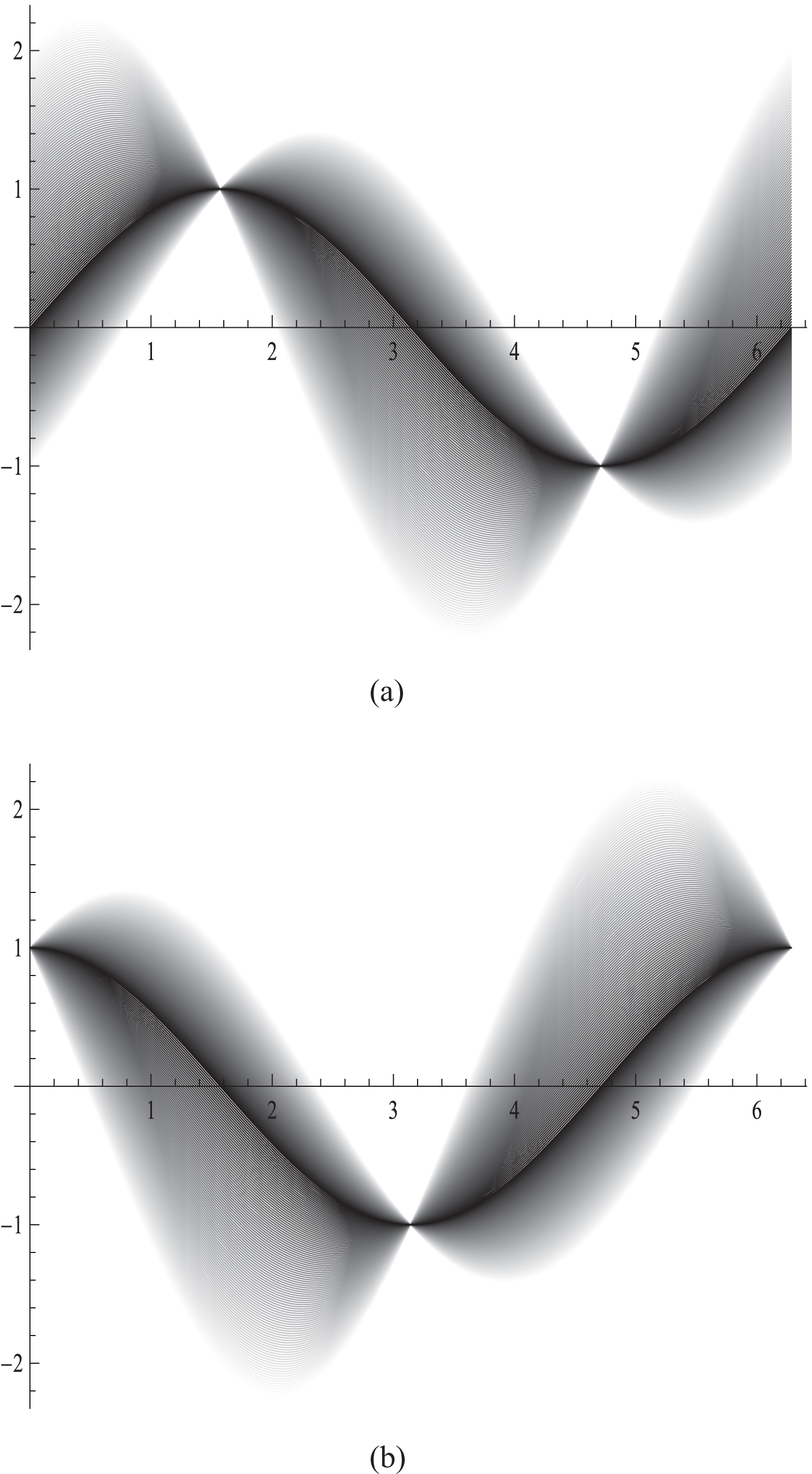
Example 6. Let A = (-1 ; 0 ;2) be a non-symmetric triangle fuzzy number and let f (t) = cos tA + sin t, t ∈ (0, 2π). Since q (t) = cos t and r (t) = sin t are differentiable on (0, 2π), it follows that f (t) is LC-differentiable on (0, 2π). Moreover, f′ (t) = q′ (t) A + r′ (t) = - sin tA + cos t. Fig. 1 shows the the grayscale images of the function f (t) and the derivative function f′ (t) in (0, 2Π), respectively.
The grayscale images of the function f (t) = cos tA + sin t (a) and the derivative function f′ (t) = - sin tA + cos t (b)
Now we will introduce the LC-differentiability of a linearly correlated fuzzy number-valued function where A is a symmetric fuzzy number.
Definition 5.5. Let be a symmetric fuzzy number with the symmetry point x∗ and let be a linearly correlated fuzzy number-valued function with the canonical form f (t) = q0 (t) A + r0 (t). For t0 ∈ (a, b), we say that f is left (right) LC-differentiable at t0 provided that the following limit
exists in the sense of the metric . Correspondingly, the limit value is called the left (right) LC-derivative of f at t0. Similarly, the left and right LC-derivative are also denoted by and , respectively.
Definition 5.6. Let be a symmetric fuzzy number with the symmetry point x∗ and let be a linearly correlated fuzzy number-valued function with the canonical form f (t) = q0 (t) A + r0 (t). For t0 ∈ (a, b), we say that f is LC-differentiable at t0 provided that f is both left and right differentiable and . Similarly, the LC-derivative is also denoted by f′ (t0).
Example 7. Let A = (-1 ; 0 ;1) be a symmetric triangle fuzzy number with the symmetry point x∗ = 0 and let be a linearly correlated fuzzy number-valued function with the canonical form f (t) = q0 (t) A + r0 (t), where
Using the definition of the LC-difference, we can obtain
Then we can infer that . By Definition 5.6, f is LC-differentiable at t = 0. However, neither nor exist.
Remark 11. Example 7 shows that the LC-differentiability of a linearly correlated fuzzy number-valued function at some point cannot be completely characterized by the differentiability of the representation functions of its canonical form, when the basic fuzzy number is symmetric. Meantime, this example also shows that the LC-differentiability is weaker than the differentiability defined by the representation functions of its canonical form in [12].
However, the following equivalence characterization of the LC-differentiability of linearly correlated fuzzy number-valued functions in a certain interval can be obtained by appending a continuity condition.
Proposition 5.2.Let be a symmetric fuzzy number with the symmetry point x∗ and let be a continuous linearly correlated fuzzy number-valued function with the canonical form f (t) = q0 (t) A + r0 (t). Then f is left (right) LC-differentiable at t0 if and only if q0 and r0 are left (right) differentiable at t0.
Proof. We only prove that f is left LC-differentiable at t0, the case for the right LC-differentiability is similar. According to the definition of the LC-difference, we can obtain
where
For the left LC-differentiability, t - t0 < 0, then we have
Necessity: If f (t) is left LC-differentiable at t0, then the left limit
Thus, the completeness of the metric space implies that there exists with α ≥ 0 such that
Therefore, we can infer from (3) that
Furthermore, it follows that
In addition, the continuity of f implies that q0 and r0 are continuous on (a, b). Then, it follows from (4) that the following two limits
exist. Therefore, we conclude that q0 and r0 are left differentiable at t0.
Sufficiency: By (2), the left differentiability of q0 and r0 implies that the limits
exist. For simplicity, we write and . Then, we get
Therefore, we can infer from (3) that
Therefore, we obtain that
By Definition 5.5, we know that f (t) is left LC-differentiable at t0.□
Corollary 5.2Let be a symmetric fuzzy number with the symmetry point x∗ and let be a continuous linearly correlated fuzzy number-valued function with the canonical form f (t) = q0 (t) A + r0 (t). Then f is LC-differentiable at t0 ∈ (a, b) if and only if q0 and r0 are both left and right differentiable at t0 and satisfy one of the following conditions
or
where () and () denote the left and right derivatives of q0 (r0) at t0, respectively.
Proof. By Definition 5.6, f is LC-differentiable at t0 ∈ (a, b) if and only if f is both left and right differentiable at t0 and . Using the proof of Proposition 5.3, we can obtain
where α and β are given as in (4), and are given by
Then, the relation is equivalent to
Obviously, we have . The following proof will be divided into five cases:
Case 1: If , then . By (2), we have . Then the condition (i) holds true.
Case 2: If , then there exists δ > 0 such that
By (2), we can obtain
Thus, the condition (i) is true.
Case 3: If , the proof is similar to Case 2.
Case 4: If , then there exists δ > 0 such that
From (2), it follows that
which means the condition (ii) holds true.
Case 5: If , the proof is similar to Case 4. □
Remark 12. From the proof of Corollary 5.4, it is easy to see that the canonical form of the derivative f′ (t0) is f′ (t0) = q1 (t0) A + r1 (t0), where
Similarly, q1 (t0) and r1 (t0) can also be defined by and .
Remark 13. When is a symmetric fuzzy number, the Corollary 5.4 shows that the differentiability of q0 and r0 is a sufficient but not necessary condition for the LC-differentiability of a continuous linearly fuzzy number-valued function f. The equivalence characterization of the LC-differentiability is consistent with the result (Proposition 4.6) in [12]. It should be noted that q1 and r1 in the canonical form f′ (t0) can also be defined by and . In addition, the differentiability of f on the interval I can be similarly defined as in Remark 10 provided that A is a symmetric fuzzy number. By Corollary 4.6, for an LC-differentiable linearly fuzzy number-valued function f on I, the LC-derivative f′ (t) and the gH-derivative coincides, that is, .
Example 8. Let A = (0 ; 1 ;2) be a symmetric triangle fuzzy number with the symmetry point x∗ = 1 and let f (t) = q (t) A + r (t) = tA + cos t, t ∈ (- π, π). By Definition 5.3, the canonical form of f is f (t) = q0 (t) + r0 (t), where
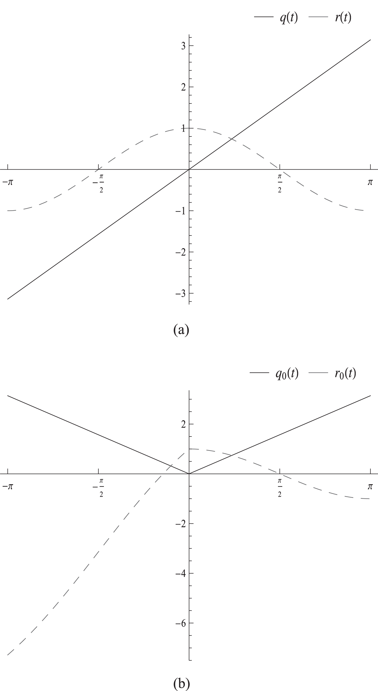
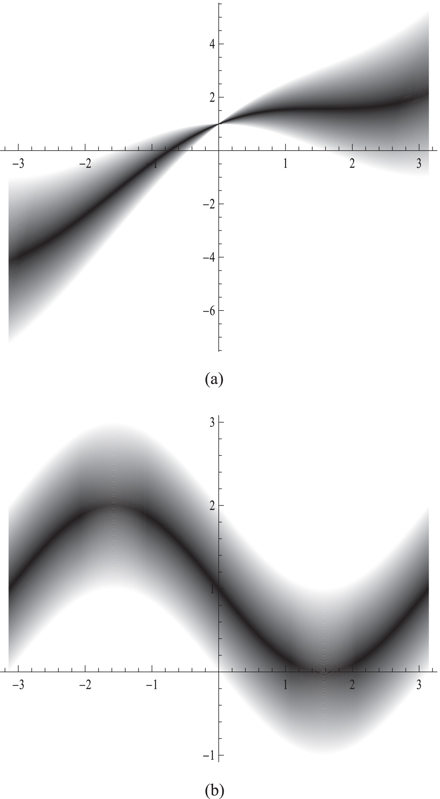
Fig. 2 shows the representation functions q and r of the function f (t) = q (t) A + r (t) and the representation functions q0 and r0 of the canonical form f (t) = q0 (t) A + r0 (t). Obviously, q0 and r0 are both left and right differentiable at t = 0, and , and . Then q0 and r0 satisfy the condition (ii) of Corollary 5.4. Hence we know that f is differentiable at t = 0 and f′ (0) = A + 3. Furthermore, we conclude that f is differentiable on (- π, π) and f′ (t) = q1 (t) A + r1 (t) = A - sin t, t ∈ (- π, π). Fig. 3 shows the grayscale images of the function f (t) = tA + cos t and the derivative function f′ (t) = A - sin t in (- π, π), respectively.
The representation functions q and r of the function f (t) = q (t) A + r (t) (a) and the representation functions q0 and r0 of the canonical form f (t) = q0 (t) A + r0 (t) (b).
The grayscale images of the function f (t) = tA + cos t (a) and the derivative function f′ (t) = A - sin t (b).
Interval-valued functions are essentially special cases of symmetric fuzzy number-valued functions, then we can also consider the differentiability of these types of functions. According to Proposition 4.5, the LC-derivative f′ (t) and the gH-derivative are coincident. Let be an interval number with the symmetry point and let be an interval-valued function with f (t) = [f1 (t) , f2 (t)], where f1 (t) ≤ f2 (t). By Proposition 4.3, f (t) can be written as the canonical form f (t) = q0 (t) A + r0 (t), where
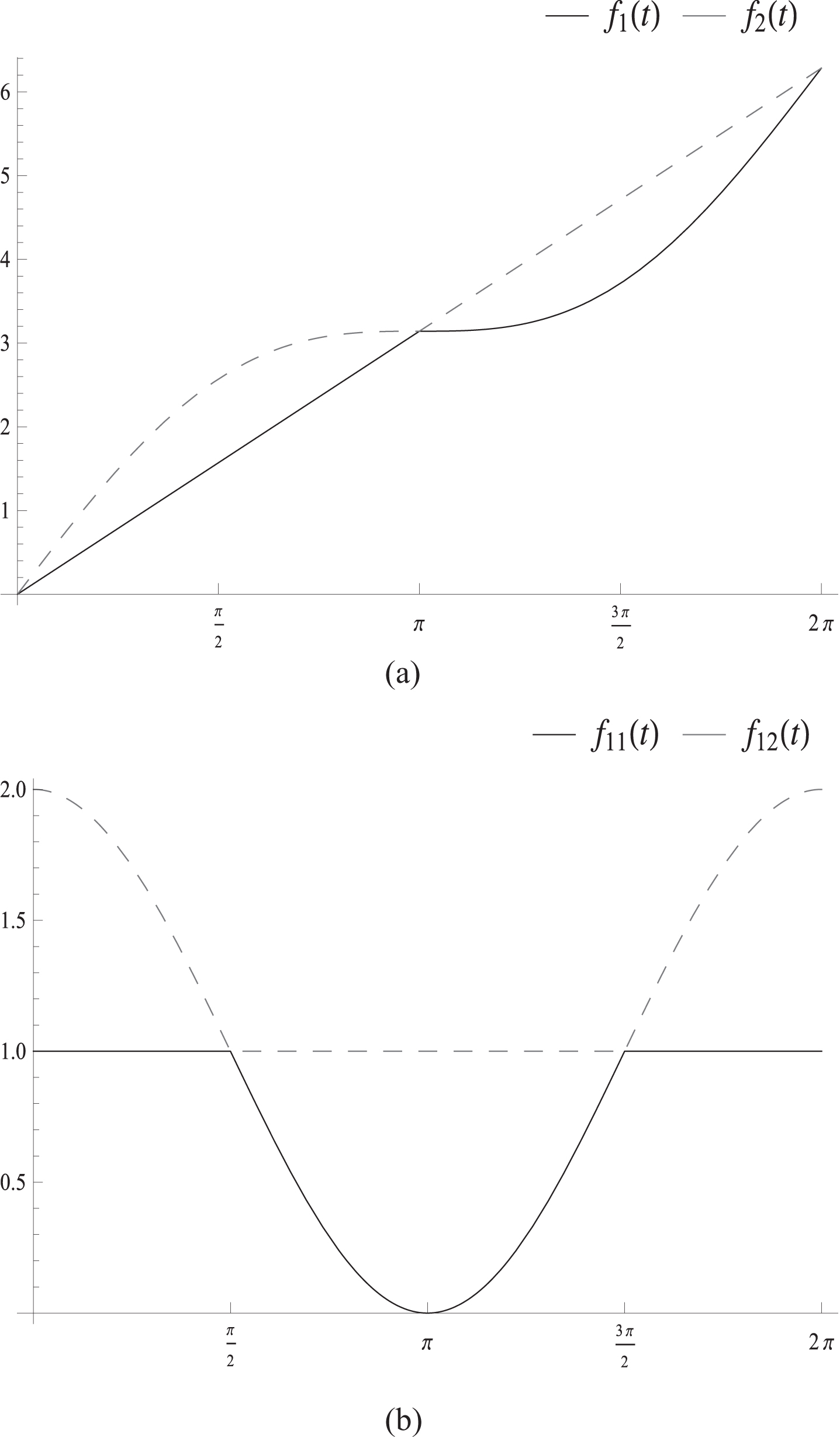
Example 9. Let A = [-1, 1] be an interval number with the symmetry point and let f (t) = [f1 (t) , f2 (t)] be an interval-valued function on (0, 2π), where
By (5), we can obtain
Then the canonical form of f is . Obviously, q0 (t) and r0 (t) are both left and right differentiable on (0, 2π). Furthermore, we get
Hence, the derivative function , where
Fig. 4. shows the boundary curves of the interval-valued function and the derivative function .
The boundary curves of the interval-valued function f (t) = [f1 (t) , f2 (t)] (a) and the boundary curves of the derivative function f′ (t) = [f11 (t) , f12 (t)] (b).
Conclusion
In this paper, two appropriate metrics were introduced in the set of A-linearly correlated fuzzy numbers depended on whether A is a symmetric fuzzy number. For the case where A is non-symmetric, there exists a linear isomorphism ΨA between and the set of A-linearly correlated fuzzy numbers. The addition and the scalar multiplication were defined by using the linear isomorphism ΨA. Then constituted a complete normed linear space. When A is a symmetric fuzzy number, the bijection was introduced from the quotient set to . Similar to the case where A is non-symmetric, the addition and the multiplication were also introduced by means of the bijection . However, the subtraction induced by the addition and the scalar multiplication in does not meet some basic needs, such as . For this reason, the notion of LC-difference of linearly correlated fuzzy numbers was introduced with the help of the operators ΨA and , respectively. In essence, the LC-difference is consistent with the difference induced by the addition and the scalar multiplication if A is non-symmetric. However, two types of differences are different if A is symmetric. Coincidentally, this difference is consistent with the generalized Hukuhara difference (gH-difference) introduced in [13] for symmetrical fuzzy numbers, especially for interval numbers. Naturally, a novel derivative for linearly correlated fuzzy number-valued functions was introduced. The equivalence characterization for the LC-differentiability of linearly correlated fuzzy number-valued functions indicate that this derivative is essentially equivalent to the derivative introduced in [12]. Besides, two equivalent characterizations of the LC-differentiability for linearly correlated fuzzy number-valued functions were established. For the non-symmetric case, the LC-differentiability of a linearly correlated fuzzy number-valued function is equivalent to the differentiability of its representation functions. For the symmetric case, a continuity condition needs to be attached to the representation function of its canonical form. Finally, it should be noted that this derivative is consistent with the gH-derivative for symmetric fuzzy number-valued functions and interval-valued functions. Compared with the gH-derivative, an important advantage is that we do not need to find the switching point when checking the differentiability of the fuzzy number-valued function. Indeed, these results will provide more options for solving fuzzy differential equations.
Footnotes
Acknowledgments
This work was supported by the National Natural Science Foundation of China (No. 11701425), the Science and Technology Planning Project of Gansu Province (No. 21JR1RE287) and the Fuxi Scientific Research Innovation Team of Tianshui Normal University (No. FXD2020-03).
References
1.
BarrosL.C. and PedroF.S., Fuzzy differential equations with interactive derivative, Fuzzy Sets Syst309 (2017), 64–80.
2.
BedeB. and GalS.G., Generalizations of the differentiability offuzzy-number-valued functions with applications to fuzzydifferential equations, Fuzzy Sets Syst151 (2005), 581–599.
CarlssonC., FullérR. and MajlenderP., Additions of completelycorrelated fuzzy numbers, in: Proceedings of the 2004 IEEEInternational Conference on Fuzzy Systems1 (2004), 535–539.
5.
EsmiE., PedroF.S., BarrosL.C. and LodwickW., Fréchetderivative for linearly correlated fuzzy function, Inform.Sciences435 (2018), 150–160.
6.
GomesL.T. and BarrosL.C., A note on the generalized difference andthe generalized differentiability, Fuzzy Sets Syst280(2015), 142–145.
PedroF.S., BarrosL.C. and EsmiE., Population growth model viainteractive fuzzy differential equation, Inform. Sciences481 (2019), 160–173.
9.
PedroF.S., EsmiE. and BarrosL.C., Calculus for linearlycorrelated fuzzy function using Fréchet derivative and Riemannintegral, Inform. Sciences512 (2020), 219–237.
10.
PuriM.L. and RalescuD.A., Differentials of fuzzy functions, J Math Anal Appl91 (1983), 552–558.
11.
NguyenH.T., A note on the extension principle for fuzzy sets, J Math Anal Appl64 (1978), 369–380.