Mehar approach to solve fuzzy linear fractional minimal cost flow problems

Abstract

To the best of author’s knowledge, only one approach is proposed in the literature to solve fuzzy linear fractional minimal cost flow problems (minimal cost flow problems in which each known arc cost is represented either by a triangular fuzzy number or a trapezoidal fuzzy number). In this paper, the mathematical incorrect assumptions, considered in the existing approach to solve fuzzy linear fractional minimal cost flow problems, are pointed out. Also, by generalizing an existing approach for solving fuzzy linear fractional programming problems, an approach (named as Mehar approach) is proposed to solve fuzzy linear fractional minimal cost flow problems. Furthermore, two numerical examples are solved to illustrate the proposed Mehar approach.

Keywords

Linear fractional minimal cost flow problem triangular fuzzy numbers trapezoidal fuzzy numbers lexicographic approach

1 Introduction

A minimal cost flow problem is one of the most practical problems in network flows [1]. The aim of a minimal cost flow problem is to determine the optimal quantity of the commodity which is to be transported through a network to minimize the total flow cost.

The fractional minimal cost flow problem is one of the generalized forms of a minimal cost flow problem. It is pertinent to mention that all the existing methods [2, 3] for solving linear fractional minimal cost flow problems are proposed by considering the assumption that the precise value of each parameter is known. However, it is not a realistic assumption as in real-life situations, some or all the parameters may not be known precisely due to unmanageable factors such as weather, social or economic conditions. Due to the same reasons, various ways have been proposed in the literature to deal with such imprecise parameters. Fuzzy set [4] is one of the ways to deal with such imprecise parameters. In the last few years, fuzzy set has been used to represent the imprecise parameters of different types of operations research problems like linear programming problems [5], linear fractional programming problems [6 –15], transportation problems [16], game theory [17] etc.

Mahmoodirad et al. [18] used a special type of fuzzy set (triangular fuzzy number or trapezoidal fuzzy number) to represent each known arc cost of a linear fractional minimal cost flow problem. Mahmoodirad et al. [18] also proposed a mathematical programming approach to solve it.

In Mahmoodirad et al.’s approach [18] firstly, a fuzzy mathematical programming problem is obtained corresponding to the considered fuzzy linear fractional minimal cost flow problem. Then, the obtained fuzzy mathematical programming problem is transformed into two equivalent crisp linearprogramming problems. Finally, the transformed crisp linear programming problems are solved to obtain an optimal solution and the fuzzy optimal value of the considered fuzzy linear fractional minimal cost flow problem.

Although, several researchers have cited Mahmoodirad et al.’s approach [18]. But, to the best of author’s knowledge, till now no one has pointed out that it is not appropriate to use Mahmoodirad et al.’s approach [18] as Mahmoodirad et al. [18] have used some mathematical incorrect assumptions in their proposed approach.

In this paper, some mathematical incorrect assumptions, considered in Mahmoodirad et al.’s approach [18] are pointed out. Also, by generalizing the existing approach [10], an approach (named as Mehar approach) is proposed to solve existing fuzzy linear fractional minimal cost flow problems [18]. Furthermore, the exact results of the fuzzy linear fractional minimal cost flow problem, considered by Mahmoodirad et al. [18] to illustrate their proposed approach, have been obtained by the proposed Mehar approach.

This paper is organized as follows: In Section 2, some basic concepts related to fuzzy set theory is reviewed. In Section 3, the linear programming formulation of a linear fractional minimal cost flow problem has been discussed. In Section 4, Mahmoodirad et al.’s approach [18] to solve fuzzy linear fractional minimal cost flow problems has been discussed. In Section 5, the mathematical incorrect assumptions, considered in Mahmoodirad et al.’s approach [18], have been pointed out. In Section 6, by generalizing the existing approach [10] an approach (named as Mehar approach) is proposed to solve existing fuzzy linear fractional minimal cost flow problems [18]. In Section 7, the exact results of the fuzzy linear fractional minimal cost flow problems, considered by Mahmoodirad et al. [18] to illustrate their proposed approach, have been obtained by the proposed Mehar approach. Section 8 concludes the paper.

2 Preliminaries

In this section, some basic definitions are reviewed [20, 21].

Definition 1 [20]. Let X be a universal set. Then, the set $\tilde{A} = {〈 x, μ_{\tilde{A}} (x) 〉 : x \in X}$ is said to be a fuzzy set defined over the universal set X, where $μ_{\tilde{A}} : X \to [0, 1]$ is said to be the membership function and the value $μ_{\tilde{A}} (x)$ is called the degree of membership for x belongs to the set $\tilde{A}$ .

Definition 2 [20]. Let $\tilde{A}$ be a fuzzy set defined over the universal set X and α ∈ (0, 1]. Then, the crisp set $A_{α} = {x \in X : μ_{\tilde{A}} (x) ⩾ α}$ is said to be the α-cut of the fuzzy set $\tilde{A}$ .

Definition 3 [20]. Let $\tilde{A}$ be a fuzzy set defined over the universal set X. Then, the crisp set $S (\tilde{A}) = {x \in X : μ_{\tilde{A}} (x) > 0}$ is said to be the support of the fuzzy set $\tilde{A}$ .

Definition 4 [20]. Let $\tilde{A}$ be a fuzzy set defined over the universal set X. Then, the crisp number $h (\tilde{A}) = sup_{x \in X} μ_{\tilde{A}} (x)$ is said to be the height of the fuzzy set $\tilde{A}$ . If $h (\tilde{A}) = 1$ , then the fuzzy set $\tilde{A}$ is said to be a normal fuzzy set.

Definition 5 [20]. A fuzzy set $\tilde{A}$ defined over the set of real numbers is said to be fuzzy number if it satisfies the following conditions

$\tilde{A}$ is normal,

A_α is a closed interval for every α ∈ (0, 1],

The support of $\tilde{A}$ is bounded.

Definition 6 [20]. A fuzzy number $\tilde{A} = (a_{1}, a_{2}, a_{3})$ is said to be triangular fuzzy number if its membership function is defined as $μ_{\tilde{A}} (x) = {\begin{matrix} 0, x < a_{1}, x > a_{3}, \\ \frac{x - a_{1}}{a_{2} - a_{1}}, a_{1}, \leq x \leq a_{2}, \\ \frac{a_{3} - x}{a_{3} - a_{2}}, a_{2} < x \leq a_{3} \end{matrix}$

Definition 7 [21]. A triangular fuzzy number $\tilde{A} = (a_{1}, a_{2}, a_{3})$ is said to be a non-negative triangular fuzzy number if and only if a₁ ⩾ 0.

Definition 8 [21]. A triangular fuzzy number $\tilde{A} = (a_{1}, a_{2}, a_{3})$ is said to be a positive triangular fuzzy number if and only if a₁ > 0.

Definition 9 [21]. Let $\tilde{A} = (a_{1}, a_{2}, a_{3})$ and $\tilde{B} = (b_{1}, b_{2}, b_{3})$ be two triangular fuzzy numbers, then $\tilde{A} \oplus \tilde{B} = (a_{1} + b_{1}, a_{2} + b_{2}, a_{3} + b_{3})$ .

Definition 10 [21]. Let $\tilde{A} = (a_{1}, a_{2}, a_{3})$ be non-negative triangular fuzzy number and k > 0, then $k \tilde{A} = ({ka}_{1}, {ka}_{2}, {ka}_{3})$ .

Definition 11 [21]. Let $\tilde{A} = (a_{1}, a_{2}, a_{3})$ and $\tilde{B} = (b_{1}, b_{2}, b_{3})$ be two non-negative triangular fuzzy numbers, then $\tilde{A} \otimes \tilde{B} = (a_{1} b_{1}, a_{2} b_{2}, a_{3} b_{3})$ .

Definition 12 [21]. Let $\tilde{A} = (a_{1}, a_{2}, a_{3})$ be a non-negative triangular fuzzy number and $\tilde{B} = (b_{1}, b_{2}, b_{3})$ be a positive triangular fuzzy number, then $\frac{\tilde{A}}{\tilde{B}} = (\frac{a_{1}}{b_{3}}, \frac{a_{2}}{b_{2}}, \frac{a_{3}}{b_{1}})$ .

Definition 13 [21]. Let $\tilde{A} = (a_{1}, a_{2}, a_{3})$ be a non-negative triangular fuzzy number, then the α-cut of the fuzzy set $\tilde{A}$ is given by A_α = [a₁ + α (a₂ - a₁) , a₃ - α (a₃ - a₂)].

Definition 14 [20]. A fuzzy number $\tilde{A} = (a_{1}, a_{2}, a_{3}, a_{4})$ is said to be trapezoidal fuzzy number if its membership function is defined as $μ_{\tilde{A}} (x) = {\begin{matrix} \begin{matrix} 0, x < a_{1}, x > a_{4}, \\ \frac{x - a_{1}}{a_{2} - a_{1}}, a_{1} \leq x < a_{2}, \\ 1, a_{2} \leq x \leq a_{3}, \end{matrix} \\ \frac{a_{4} - x}{a_{4} - a_{3}}, a_{3} < x \leq a_{4} \end{matrix}$

Definition 15 [21]. A trapezoidal fuzzy number $\tilde{A} = (a_{1}, a_{2}, a_{3}, a_{4})$ is said to be a non-negative trapezoidal fuzzy number if and only if a₁ ⩾ 0.

Definition 16 [21]. A trapezoidal fuzzy number $\tilde{A} = (a_{1}, a_{2}, a_{3}, a_{4})$ is said to be a positive trapezoidal fuzzy number if and only if a₁ > 0.

Definition 17 [21]. Let $\tilde{A} = (a_{1}, a_{2}, a_{3}, a_{4})$ and $\tilde{B} = (b_{1}, b_{2}, b_{3}, b_{4})$ be two trapezoidal fuzzy numbers, then $\tilde{A} \oplus \tilde{B} = (a_{1} + b_{1}, a_{2} + b_{2}, a_{3} + b_{3} + a_{4} + b_{4})$ .

Definition 18 [21]. Let $\tilde{A} = (a_{1}, a_{2}, a_{3}, a_{4})$ be non-negative trapezoidal fuzzy number and k > 0, then $k \tilde{A} = ({ka}_{1}, {ka}_{2}, {ka}_{3}, {ka}_{4})$ .

Definition 19 [21]. Let $\tilde{A} = (a_{1}, a_{2}, a_{3}, a_{4})$ and $\tilde{B} = (b_{1}, b_{2}, b_{3}, b_{4})$ be two non-negative trapezoidal fuzzy numbers, then $\tilde{A} \otimes \tilde{B} = (a_{1} b_{1}, a_{2} b_{2}, a_{3} b_{3}, a_{4} b_{4})$ .

Definition 20 [21]. Let $\tilde{A} = (a_{1}, a_{2}, a_{3}, a_{4})$ be a non-negative trapezoidal fuzzy number and $\tilde{B} = (b_{1}, b_{2}, b_{3}, b_{4})$ be a positive trapezoidal fuzzy number, then $\frac{\tilde{A}}{\tilde{B}} = (\frac{a_{1}}{b_{4}}, \frac{a_{2}}{b_{3}}, \frac{a_{3}}{b_{2}}, \frac{a_{4}}{b_{1}})$ .

Definition 21 [21]. Let $\tilde{A} = (a_{1}, a_{2}, a_{3}, a_{4})$ be a non-negative trapezoidal fuzzy number, then the α-cut of the fuzzy set $\tilde{A}$ is given by A_α = [a₁ + α (a₂ - a₁) , a₄ - α (a₄ - a₃)].

3 Linear fractional minimal cost flow programming problem corresponding to a linear fractional minimal cost flow problem

The minimal cost flow problem is a fundamental network flow problem. The aim of the minimal cost problem is to determine the least cost shipment of a commodity through a network in order to satisfy demands at certain vertices from available supplies at other vertices. This model has a number of applications, e.g., the distribution of a product from manufacturing plants to warehouses or from warehouses to retailers, the flow of raw material and intermediate goods through the various machining stations in a production line, the routing of automobiles through an urban street network, and the routing of calls through the telephone system [1].

An optimal solution of a linear minimal cost flow problem consisting of a non-empty set V of vertices and a set E disjoint from V as the set of arcs, can be obtained by solving its equivalent linear programming problem (P₁) [1].

Problem ( P₁)

Minimize (∑_(i,j)∈Ec_ijx_ij)

Subject to

∑_(i,j)∈Ex_ij -∑_(j,i)∈Ex_ji = b_i ∀ i ∈ { 1, 2, …, m }

l_ij ⩽ x_ij ⩽ u_ij ∀ (i, j) ∈ E

where,

x_ij represents the amount of flow on the arc (i, j).

b_i represents the difference between the amount sent from vertex i and the amount received by this vertex.

c_ij represents the cost for transporting one unit quantity of the commodity across the arc (i, j).

l_ij represents the lower bound capacity of the arc (i, j) ∈ E.

u_ij represents the upper bound capacity of the arc (i, j) ∈ E.

If it is assumed that the aim of a minimal cost flow problem is to minimize the efficiency of some activity, e.g., cost of production per unit of produced goods, instead of determining the least cost shipment of a commodity. Then, such a minimal cost flow problem is known as linear fractional minimal cost flow problem.

An optimal solution of a linear fractional minimal cost flow problem consisting of a non-empty set V of vertices and a set E disjoint from V as the set of arcs, can be obtained by solving its equivalent linear fractional programming problem (P₂).

Problem (P₂)

$Minimize (\frac{\sum_{(i, j) \in E} c_{ij} x_{ij} + γ}{\sum_{(i, j) \in E} d_{ij} x_{ij} + β})$

Subject to

∑_(i,j)∈Ex_ij -∑_(j,i)∈Ex_ji = b_i ∀ i ∈ { 1, 2, …, m }

l_ij ⩽ x_ij ⩽ u_ij ∀ (i, j) ∈ E

where,

d_ij represents the profit for transporting one unit quantity of the commodity across the arc (i, j).

γ and β are given constants.

It is obvious from the problem (P₁) and the problem (P₂) that in the problem (P₁), the objective function is a linear function. While, in the problem (P₂), the objective function is the ratio of two linear functions i.e., to find an optimal solution of a linear minimal cost flow problem, there is a need to solve the linear programming problem (P₁). While, to find an optimal solution of the linear fractional minimal cost flow problem, there is a need to solve the linear fractional programming problem (P₂). It is a well-known fact that much computational efforts are required to solve a crisp linear fractional programming problem as compared to a crisp linear programming problem. Therefore, much computational efforts are required to solve a linear fractional minimal cost flow problem as compared to a linear minimal costproblem.

4 Mahmoodirad et al.’s approach for solving fuzzy linear fractional minimal cost flow problems

The aim of Mahmoodirad et al. [18] was to propose an approach to solve such linear fractional minimal cost flow problems in which each known arc cost is either represented by a triangular fuzzy number or a trapezoidal fuzzy number. To achieve this aim, Mahmoodirad et al. [18] firstly, obtained the fuzzy linear fractional minimal cost flow programming problem (P₃) by either replacing each known arc costs c_ij and d_ij of the linear fractional programming problem (P₂) with triangular fuzzy numbers ${\tilde{c}}_{ij} = (c_{ij 1}, c_{ij 2}, c_{ij 3})$ and ${\tilde{d}}_{ij} = (d_{ij 1}, d_{ij 2}, d_{ij 3})$ respectively or with trapezoidal fuzzy numbers ${\tilde{c}}_{ij} = (c_{ij 1}, c_{ij 2}, c_{ij 3}, c_{ij 4})$ and ${\tilde{d}}_{ij} = (d_{ij 1}, d_{ij 2}, d_{ij 3}, d_{ij 4})$ respectively.

Problem (P₃)

$Minimize (\frac{\sum_{(i, j) \in E} {\tilde{c}}_{ij} x_{ij} + γ}{\sum_{(i, j) \in E} {\tilde{d}}_{ij} x_{ij} + β})$

Subject to

Constraints of the problem (P₂).

Then, Mahmoodirad et al. [18] used the following steps to solve the fuzzy linear fractional programming problem (P₃).

Step 1: Transform the fuzzy linear fractional programming problem (P₃) into its equivalent crisp mathematical programming problems (P₄) and(P₅).

Problem (P₄)

$Z_{α}^{L} = min_{\begin{matrix} {(C_{ij})}_{α}^{L} ⩽ c_{ij} ⩽ {(C_{ij})}_{α}^{U} \\ {(D_{ij})}_{α}^{L} ⩽ d_{ij} ⩽ {(D_{ij})}_{α}^{U} \\ \forall (i, j) \in E \end{matrix}} [min (\frac{\sum_{(i, j) \in E} c_{ij} x_{ij} + γ}{\sum_{(i, j) \in E} d_{ij} x_{ij} + β})]$

Subject to

Constraints of the problem (P₂).

where,

${(C_{ij})}_{α}^{L}$ is the lower bound of the α-cut for the fuzzy number ${\tilde{c}}_{ij}$ .

${(C_{ij})}_{α}^{U}$ is the upper bound of the α-cut for the fuzzy number ${\tilde{c}}_{ij}$ .

${(D_{ij})}_{α}^{L}$ is the lower bound of the α-cut for the fuzzy number ${\tilde{d}}_{ij}$ .

${(D_{ij})}_{α}^{U}$ is the upper bound of the α-cut for the fuzzy number ${\tilde{d}}_{ij}$ .

Problem (P₅)

$Z_{α}^{U} = max_{\begin{matrix} {(C_{ij})}_{α}^{L} ⩽ c_{ij} ⩽ {(C_{ij})}_{α}^{U} \\ {(D_{ij})}_{α}^{L} ⩽ d_{ij} ⩽ {(D_{ij})}_{α}^{U} \\ \forall (i, j) \in E \end{matrix}} [min (\frac{\sum_{(i, j) \in E} c_{ij} x_{ij} + γ}{\sum_{(i, j) \in E} d_{ij} x_{ij} + β})]$

Subject to

Constraints of the problem (P₂).

Step 2: Use the following steps to transform the crisp mathematical fractional programming problem (P₄) into its equivalent crisp linear programmingproblem.

Step 2a: Transform the crisp mathematical fractional programming problem (P₄) into its equivalent crisp mathematical fractional programming problem (P₆).

Problem (P₆)

$Z_{α}^{L} = min (\frac{\sum_{(i, j) \in E} c_{ij} x_{ij} + γ}{\sum_{(i, j) \in E} d_{ij} x_{ij} + β})$

Subject to

∑_(i,j)∈Ex_ij -∑_(j,i)∈Ex_ji = b_i ∀ i ∈ { 1, 2, …, m }

l_ij ⩽ x_ij ⩽ u_ij ∀ (i, j) ∈ E

${(C_{ij})}_{α}^{L} ⩽ c_{ij} ⩽ {(C_{ij})}_{α}^{U} \forall (i, j) \in E$

${(D_{ij})}_{α}^{L} ⩽ d_{ij} ⩽ {(D_{ij})}_{α}^{U} \forall (i, j) \in E$

Step 2b: Transform the crisp mathematical fractional programming problem (P₆) into its equivalent crisp mathematical programming problem (P₇).

Problem (P₇)

$Z_{α}^{L} = min (\sum_{(i, j) \in E} c_{ij} y_{ij} + γ t)$

Subject to

∑_(i,j)∈Ey_ij -∑_(j,i)∈Ey_ji = b_it ∀ i ∈ { 1, 2, …, m }

∑_(i,j)∈Ed_ijy_ij + βt = 1

l_ijt ⩽ y_ij ⩽ u_ijt ∀ (i, j) ∈ E

${(C_{ij})}_{α}^{L} ⩽ c_{ij} ⩽ {(C_{ij})}_{α}^{U} \forall (i, j) \in E$

${(D_{ij})}_{α}^{L} ⩽ d_{ij} ⩽ {(D_{ij})}_{α}^{U} \forall (i, j) \in E$

t > 0.

Step 2c: Transform the crisp mathematical programming problem (P₇) into its equivalent crisp mathematical programming problem (P₈).

Problem (P₈)

$Z_{α}^{L} = min (\sum_{(i, j) \in E} {(C_{ij})}_{α}^{L} y_{ij} + γ t)$

Subject to

∑_(i,j)∈Ey_ij -∑_(j,i)∈Ey_ji = b_it ∀ i ∈ { 1, 2, …, m }

∑_(i,j)∈Ed_ijy_ij + βt = 1

l_ijt ⩽ y_ij ⩽ u_ijt ∀ (i, j) ∈ E

${(D_{ij})}_{α}^{L} ⩽ d_{ij} ⩽ {(D_{ij})}_{α}^{U} \forall (i, j) \in E$

t > 0.

Step 2d: Transform the crisp mathematical programming problem (P₈) into its equivalent crisp linear programming problem (P₉).

Problem (P₉)

$Z_{α}^{L} = min (\sum_{(i, j) \in E} {(C_{ij})}_{α}^{L} y_{ij} + γ t)$

Subject to

∑_(i,j)∈Ey_ij -∑_(j,i)∈Ey_ji = b_it ∀ i ∈ { 1, 2, …, m }

∑_(i,j)∈Eρ_ij + βt = 1

l_ijt ⩽ y_ij ⩽ u_ijt ∀ (i, j) ∈ E

${(D_{ij})}_{α}^{L} y_{ij} ⩽ ρ_{ij} ⩽ {(D_{ij})}_{α}^{U} y_{ij} \forall (i, j) \in E$

t > 0.

Step 3: Use the following steps to transform the crisp mathematical programming problem (P₅) into its equivalent crisp linear programming problem.

Step 3a: Transform the crisp mathematical programming problem (P₅) into its equivalent crisp mathematical programming problem (P₁₀).

Problem (P₁₀)

Subject to

∑_(i,j)∈Ey_ij -∑_(j,i)∈Ey_ji = b_it ∀ i ∈ { 1, 2, …, m }

∑_(i,j)∈Ed_ijy_ij + βt = 1

l_ijt ⩽ y_ij ⩽ u_ijt ∀ (i, j) ∈ E

t > 0.

Step 3b: Transform the crisp mathematical programming problem (P₁₀) into its equivalent crisp mathematical programming problem (P₁₁).

Problem (P₁₁)

$Z_{α}^{U} = max p$

Subject to

π_i - π_j + d_ijp + s_ij - n_ij ⩽ c_ij ∀ (i, j) ∈ E

$\sum_{i = 1}^{m} (- b_{i} π_{i}) + β p - \sum_{(i, j) \in E} l_{ij} s_{ij} + \sum_{(i, j) \in E} u_{ij} n_{ij} ⩽ γ$

${(C_{ij})}_{α}^{L} ⩽ c_{ij} ⩽ {(C_{ij})}_{α}^{U} \forall (i, j) \in E$

${(D_{ij})}_{α}^{L} ⩽ d_{ij} ⩽ {(D_{ij})}_{α}^{U} \forall (i, j) \in E$

s_ij, n_ij ⩾ 0 ∀ (i, j) ∈ E

π_i, p is unrestricted ∀i∈ { 1, 2, …, m }

Step 3c: Transform the crisp mathematical programming problem (P₁₁) into its equivalent crisp mathematical programming problem (P₁₂).

Problem (P₁₂)

$Z_{α}^{U} = max p$

Subject to

$π_{i} - π_{j} + d_{ij} p + s_{ij} - n_{ij} ⩽ {(C_{ij})}_{α}^{U} \forall (i, j) \in E$

$\sum_{i = 1}^{m} (- b_{i} π_{i}) + β p - \sum_{(i, j) \in E} l_{ij} s_{ij} + \sum_{(i, j) \in E} u_{ij} n_{ij} ⩽ γ$

${(D_{ij})}_{α}^{L} ⩽ d_{ij} ⩽ {(D_{ij})}_{α}^{U} \forall (i, j) \in E$

s_ij, n_ij ⩾ 0 ∀ (i, j) ∈ E

p > 0, π_i is unrestricted ∀i∈ { 1, 2, …, m }

Step 3d: Transform the crisp mathematical programming problem (P₁₂) into its equivalent crisp linear programming problem (P₁₃).

Problem (P₁₃)

$Z_{α}^{U} = max p$

Subject to

$π_{i} - π_{j} + w_{ij} + s_{ij} - n_{ij} ⩽ {(C_{ij})}_{α}^{U} \forall (i, j) \in E$

$\sum_{i = 1}^{m} (- b_{i} π_{i}) + β p - \sum_{(i, j) \in E} l_{ij} s_{ij} + \sum_{(i, j) \in E} u_{ij} n_{ij} ⩽ γ$

${(D_{ij})}_{α}^{L} p ⩽ w_{ij} ⩽ {(D_{ij})}_{α}^{U} p \forall (i, j) \in E$

s_ij, n_ij ⩾ 0 ∀ (i, j) ∈ E

p > 0, π_i is unrestricted ∀i∈ { 1, 2, …, m }

Step 4: Find the optimal solution {(x_ij) _α=0} and the optimal value ( $Z_{α = 0}^{L}$ ) of the crisp linear programming problem (P₉).

Step 5: Find the optimal solution {(x_ij) _α=1} and the optimal value ( $Z_{α = 1}^{L}$ ) of the crisp linear programming problem (P₉).

Step 6: Find the optimal solution {(x_ij) _α=0} and the optimal value ( $Z_{α = 0}^{U}$ ) of the crisp linear programming problem (P₁₃).

Step 7: Find the optimal solution {(x_ij) _α=1} and the optimal value ( $Z_{α = 1}^{U}$ ) of the crisp linear programming problem (P₁₃).

Step 8: Using the optimal values, obtained in Step 4 to Step 7, the obtained fuzzy optimal value is $(Z_{α = 0}^{L}, Z_{α = 1}^{L}, Z_{α = 1}^{U}, Z_{α = 0}^{U})$ .

5 Mathematical incorrect assumptions considered in Mahmoodirad et al.’s approach

In this section, some mathematical incorrect assumptions, considered in Mahmoodirad et al.’s approach [18], have been pointed out.

It is obvious from Step 2c and Step 2d of Mahmoodirad et al.’s approach [18], discussed in Section 4, that Mahmoodirad et al. [18] have assumed $c_{ij} = {(C_{ij})}_{α}^{L}$ and d_ijy_ij = ρ_ij to transform the mathematical programming problem (P₇) into the linear programming problem (P₉) i.e., Mahmoodirad et al. [18] have assumed that the mathematical programming problem (P₇) is equivalent to the linear programming problem (P₉). However, the linear programming problem (P₉) is not equivalent to the mathematical programming problem (P₇). The following also validates this claim.

In the numerical example 1, considered by Mahmoodirad et al. [18] to illustrate their proposed approach, Mahmoodirad et al. [18] have used $c_{ij} = {(C_{ij})}_{α}^{L}$ and d_ijy_ij = ρ_ij to transform the mathematical programming problem (P₁₄) into the linear programming problem (P₁₅) i.e., Mahmoodirad et al. [18] have assumed that the linear programming problem (P₁₅) is equivalent to the mathematical programming problem (P₁₄).

Problem (P₁₄)

$\begin{matrix} Z_{α}^{L} = min (c_{13} y_{13} + c_{14} y_{14} + c_{15} y_{15} + c_{23} y_{23} + \\ c_{24} y_{24} + c_{25} y_{25} + c_{34} y_{34} + c_{36} y_{36} + c_{37} y_{37} + \\ c_{45} y_{45} + c_{46} y_{46} + c_{47} y_{47} + c_{56} y_{56} + c_{57} y_{57} + 55 t) \end{matrix}$

Subject to

y₁₃ + y₁₄ + y₁₅ = 30t,

y₂₃ + y₂₄ + y₂₅ = 60t,

y₃₄ + y₃₆ + y₃₇ - y₁₃ - y₂₃ = 0,

y₄₆ + y₄₇ - y₁₄ - y₂₄ = 0,

y₅₆ + y₅₇ - y₁₅ - y₂₅ = 0,

-y₃₆ - y₄₆ - y₅₆ = -20t,

-y₃₇ - y₄₇ - y₅₇ = -70t,

$\begin{matrix} d_{13} y_{13} + d_{14} y_{14} + d_{15} y_{15} + d_{23} y_{23} + d_{24} y_{24} + \\ d_{25} y_{25} + d_{34} y_{34} + d_{36} y_{36} + d_{37} y_{37} + d_{45} y_{45} + \\ d_{46} y_{46} + d_{47} y_{47} + d_{56} y_{56} + d_{57} y_{57} + 60 t = 1 \end{matrix}$

0 ⩽ y₁₃ ⩽ 40t, 0 ⩽ y₁₄ ⩽ 10t,

0 ⩽ y₁₅ ⩽ 15t, 0 ⩽ y₂₃ ⩽ 50t,

0 ⩽ y₂₄ ⩽ 80t, 0 ⩽ y₂₅ ⩽ 40t,

0 ⩽ y₃₄ ⩽ 20t, 0 ⩽ y₃₆ ⩽ 100t,

0 ⩽ y₃₇ ⩽ 90t, 0 ⩽ y₄₅ ⩽ 15t,

0 ⩽ y₄₆ ⩽ 30t, 0 ⩽ y₄₇ ⩽ 20t,

0 ⩽ y₅₆ ⩽ 15t, 0 ⩽ y₅₇ ⩽ 100t,

(5 + 35α) ⩽ c₁₃ ⩽ (90 - 50α) ,

(4 + 41α) ⩽ c₁₄ ⩽ (115 - 70α) ,

(5 + 52α) ⩽ c₁₅ ⩽ (116 - 59α) ,

(10 + 30α) ⩽ c₂₃ ⩽ (85 - 45α) ,

(10 + 40α) ⩽ c₂₄ ⩽ (120 - 70α) ,

(13 + 47α) ⩽ c₂₅ ⩽ (164 - 104α) ,

(2 + 8α) ⩽ c₃₄ ⩽ (25 - 15α) ,

(8 + 42α) ⩽ c₃₆ ⩽ (145 - 95α) ,

(2 + 33α) ⩽ c₃₇ ⩽ (105 - 70α) ,

(3 + 7α) ⩽ c₄₅ ⩽ (40 - 30α) ,

(8 + 32α) ⩽ c₄₆ ⩽ (115 - 75α) ,

(5 + 20α) ⩽ c₄₇ ⩽ (56 - 31α) ,

(5 + 25α) ⩽ c₅₆ ⩽ (75 - 45α) ,

(2 + 8α) ⩽ c₅₇ ⩽ (40 - 30α) ,

(20 + 10α) ⩽ d₁₃ ⩽ (50 - 20α) ,

(30 + 10α) ⩽ d₁₄ ⩽ (60 - 20α) ,

(60 + 20α) ⩽ d₁₅ ⩽ (100 - 20α) ,

(5 + 65α) ⩽ d₂₃ ⩽ (80 - 10α) ,

(80 + 10α) ⩽ d₂₄ ⩽ (100 - 10α) ,

(50 + 10α) ⩽ d₂₅ ⩽ (60 - 10α) ,

(90 + 20α) ⩽ d₃₄ ⩽ (120 - 10α) ,

(70 + 10α) ⩽ d₃₆ ⩽ (100 - 20α) ,

(10 + 20α) ⩽ d₃₇ ⩽ (40 - 10α) ,

(20 + 10α) ⩽ d₄₅ ⩽ (40 - 10α) ,

(40 + 20α) ⩽ d₄₆ ⩽ (80 - 20α) ,

(80 + 10α) ⩽ d₄₇ ⩽ (110 - 20α) ,

(20 + 20α) ⩽ d₅₆ ⩽ (60 - 20α) ,

(40 + 10α) ⩽ d₅₇ ⩽ (60 - 10α) ,

t > 0.

Problem (P₁₅)

$\begin{matrix} Z_{α}^{L} = min [(5 + 35 α) y_{13} + (4 + 41 α) y_{14} + (5 + \\ 52 α) y_{15} + (10 + 30 α) y_{23} + (10 + 40 α) y_{24} + \\ (13 + 47 α) y_{25} + (2 + 8 α) y_{34} + (8 + 42 α) y_{36} + \\ (2 + 33 α) y_{37} + (3 + 7 α) y_{45} + (8 + 32 α) y_{46} + \\ (5 + 20 α) y_{47} + (5 + 25 α) y_{56} + (2 + 8 α) y_{57} + 55 t] \end{matrix}$

Subject to

y₁₃ + y₁₄ + y₁₅ = 30t,

y₂₃ + y₂₄ + y₂₅ = 60t,

y₃₄ + y₃₆ + y₃₇ - y₁₃ - y₂₃ = 0,

y₄₆ + y₄₇ - y₁₄ - y₂₄ = 0,

y₅₆ + y₅₇ - y₁₅ - y₂₅ = 0,

-y₃₆ - y₄₆ - y₅₆ = -20t,

-y₃₇ - y₄₇ - y₅₇ = -70t,

$\begin{matrix} ρ_{13} + ρ_{14} + ρ_{15} + ρ_{23} + ρ_{24} + ρ_{25} + ρ_{34} + ρ_{36} + \\ ρ_{37} + ρ_{45} + ρ_{46} + ρ_{47} + ρ_{56} + ρ_{57} + 60 t = 1 \end{matrix}$

0 ⩽ y₁₃ ⩽ 40t, 0 ⩽ y₁₄ ⩽ 10t,

0 ⩽ y₁₅ ⩽ 15t, 0 ⩽ y₂₃ ⩽ 50t,

0 ⩽ y₂₄ ⩽ 80t, 0 ⩽ y₂₅ ⩽ 40t,

0 ⩽ y₃₄ ⩽ 20t, 0 ⩽ y₃₆ ⩽ 100t,

0 ⩽ y₃₇ ⩽ 90t, 0 ⩽ y₄₅ ⩽ 15t,

0 ⩽ y₄₆ ⩽ 30t, 0 ⩽ y₄₇ ⩽ 20t,

0 ⩽ y₅₆ ⩽ 15t, 0 ⩽ y₅₇ ⩽ 100t,

(20 + 10α) y₁₃ ⩽ ρ₁₃ ⩽ (50 - 20α) y₁₃,

(30 + 10α) y₁₄ ⩽ ρ₁₄ ⩽ (60 - 20α) y₁₄,

(60 + 20α) y₁₅ ⩽ ρ₁₅ ⩽ (100 - 20α) y₁₅,

(5 + 65α) y₂₃ ⩽ ρ₂₃ ⩽ (80 - 10α) y₂₃,

(80 + 10α) y₂₄ ⩽ ρ₂₄ ⩽ (100 - 10α) y₂₄,

(50 + 10α) y₂₅ ⩽ ρ₂₅ ⩽ (60 - 10α) y₂₅,

(90 + 20α) y₃₄ ⩽ ρ₃₄ ⩽ (120 - 10α) y₃₄,

(70 + 10α) y₃₆ ⩽ ρ₃₆ ⩽ (100 - 20α) y₃₆,

(10 + 20α) y₃₇ ⩽ ρ₃₇ ⩽ (40 - 10α) y₃₇,

(20 + 10α) y₄₅ ⩽ ρ₄₅ ⩽ (40 - 10α) y₄₅,

(40 + 20α) y₄₆ ⩽ ρ₄₆ ⩽ (80 - 20α) y₄₆,

(80 + 10α) y₄₇ ⩽ ρ₄₇ ⩽ (110 - 20α) y₄₇,

(20 + 20α) y₅₆ ⩽ ρ₅₆ ⩽ (60 - 20α) y₅₆,

(40 + 10α) y₅₇ ⩽ ρ₅₇ ⩽ (60 - 10α) y₅₇,

t > 0.

While, in actual case, the linear programming problem (P₁₅) is not equivalent to the mathematical programming problem (P₁₄) as it is obvious from a) and b) that ρ_ij ≠ d_ijy_ij ∀ i, j e.g., ρ₁₃ = 0.01723 is not equal to d₁₃y₁₃ = 0.116. While, the condition ρ_ij = d_ijy_ij ∀ i, j has been considered to transform the mathematical programming problem (P₁₄) into the linear programming problem (P₁₅).

On solving the non-linear programming problem (P₁₄), the obtained optimal solution, for α = 0, is $\begin{matrix} c_{13} = 5, c_{14} = 23 . 8284, c_{15} = 5, c_{23} = 10, c_{24} = \\ 10, c_{25} = 23 . 13135, c_{34} = 25, c_{36} = 135.51165, \\ c_{37} = 2, c_{45} = 39 . 13285, c_{46} = 8, c_{47} = 5, c_{56} = \\ 42 . 94680, c_{57} = 16 . 82248, d_{13} = 50, d_{14} = \\ 42 . 04071, d_{15} = 70 . 86333, d_{23} = 80, d_{24} = 100, \\ d_{25} = 50 . 20785, d_{34} = 120, d_{36} = 99 . 49369, d_{37} \\ = 40, d_{45} = 38 . 63985, d_{46} = 80, d_{47} = 110, d_{56} \\ = 54 . 10267, d_{57} = 56 . 75489, y_{13} = 0 . 00232, y_{23} \\ = 0 . 00154, y_{24} = 0 . 00308, y_{37} = 0 . 00386, y_{46} = \\ 0 . 00154, y_{47} = 0 . 00154, y_{14} = y_{15} = y_{25} = y_{34} = \\ y_{36} = y_{45} = y_{56} = y_{57 =} 0, t = 0 . 0000771 and \end{matrix}$ optimal value is 0.08989.

On solving the linear programming problem (P₁₅), the obtained optimal solution, for α = 0, is $\begin{matrix} ρ_{13} = 0.01723, ρ_{14} = 0.04135, ρ_{15} = 0.10338, \\ ρ_{23} = 0.20533, ρ_{24} = 0.15684, ρ_{36} = 0.04991, \\ ρ_{37} = 0.09648, ρ_{45} = 0.04135, ρ_{46} = 0.07034, \\ ρ_{47} = 0.15162, ρ_{57} = 0.06203, ρ_{25} = ρ_{34} = ρ_{56} \\ = 0, y_{13} = 0.00034, y_{14} = 0.00069, y_{15} = 0.00103, \\ y_{23} = 0.00256, y_{24} = 0.00157, y_{36} = 0.00050, \\ y_{37} = 0.00241, y_{45} = 0.00103, y_{46} = 0.00087, \\ y_{47} = 0.00138, y_{57} = 0.00103, y_{25} = y_{34} = y_{56} \\ = 0, t = 0.00007 and optimal value is 0.08270 . \end{matrix}$

It is obvious from Step 3c and 3d of Mahmoodirad et al.’s approach [18], discussed in Section 4, that Mahmoodirad et al. [18] have assumed $c_{ij} = {(C_{ij})}_{α}^{U}$ and w_ij = d_ijp to transform the mathematical programming problem (P₁₁) into the linear programming problem (P₁₃) i.e., Mahmoodirad et al. [18] have assumed that the mathematical programming problem (P₁₁) is equivalent to the linear programming problem (P₁₃). However, the linear programming problem (P₁₃) is not equivalent to the mathematical programming problem (P₁₁).

The following also validates this claim.

In the numerical example 1, considered by Mahmoodirad et al. [18] to illustrate their proposed approach, Mahmoodirad et al. [18] have used $c_{ij} = {(C_{ij})}_{α}^{U}$ and w_ij = d_ijp to transform the mathematical programming problem (P₁₆) into the linear programming problem (P₁₇) i.e., Mahmoodirad et al. [18] have assumed that the linear programming problem (P₁₇) is equivalent to the mathematical programming problem (P₁₆).

Problem (P₁₆)

$Z_{α}^{U} = max p$

Subject to

π₁ - π₃ + d₁₃p + s₁₃ - n₁₃ ⩽ c₁₃,

π₁ - π₄ + d₁₄p + s₁₄ - n₁₄ ⩽ c₁₄,

π₁ - π₅ + d₁₅p + s₁₅ - n₁₅ ⩽ c₁₅,

π₂ - π₃ + d₂₃p + s₂₃ - n₂₃ ⩽ c₂₃,

π₂ - π₄ + d₂₄p + s₂₄ - n₂₄ ⩽ c₂₄,

π₂ - π₅ + d₂₅p + s₂₅ - n₂₅ ⩽ c₂₅,

π₃ - π₄ + d₃₄p + s₃₄ - n₃₄ ⩽ c₃₄,

π₃ - π₆ + d₃₆p + s₃₆ - n₃₆ ⩽ c₃₆,

π₃ - π₇ + d₃₇p + s₃₇ - n₃₇ ⩽ c₃₇,

π₄ - π₅ + d₄₅p + s₄₅ - n₄₅ ⩽ c₄₅,

π₄ - π₆ + d₄₆p + s₄₆ - n₄₆ ⩽ c₄₆,

π₄ - π₇ + d₄₇p + s₄₇ - n₄₇ ⩽ c₄₇,

π₅ - π₆ + d₅₆p + s₅₆ - n₅₆ ⩽ c₅₆,

π₅ - π₇ + d₅₇p + s₅₇ - n₅₇ ⩽ c₅₇,

$\begin{matrix} - 30 π_{1} - 60 π_{2} + 20 π_{6} + 70 π_{7} + 60 p + 40 n_{13} + \\ 10 n_{14} + 15 n_{15} + 50 n_{23} + 80 n_{24} + 40 n_{25} + \\ 20 n_{34} + 100 n_{36} + 90 n_{37} + 15 n_{45} + 30 n_{46} + \\ 20 n_{47} + 15 n_{56} + 100 n_{57} ⩽ 55, \end{matrix}$

(5 + 35α) ⩽ c₁₃ ⩽ (90 - 50α) ,

(4 + 41α) ⩽ c₁₄ ⩽ (115 - 70α) ,

(5 + 52α) ⩽ c₁₅ ⩽ (116 - 59α) ,

(10 + 30α) ⩽ c₂₃ ⩽ (85 - 45α) ,

(10 + 40α) ⩽ c₂₄ ⩽ (120 - 70α) ,

(13 + 47α) ⩽ c₂₅ ⩽ (164 - 104α) ,

(2 + 8α) ⩽ c₃₄ ⩽ (25 - 15α) ,

(8 + 42α) ⩽ c₃₆ ⩽ (145 - 95α) ,

(2 + 33α) ⩽ c₃₇ ⩽ (105 - 70α) ,

(3 + 7α) ⩽ c₄₅ ⩽ (40 - 30α) ,

(8 + 32α) ⩽ c₄₆ ⩽ (115 - 75α) ,

(5 + 20α) ⩽ c₄₇ ⩽ (56 - 31α) ,

(5 + 25α) ⩽ c₅₆ ⩽ (75 - 45α) ,

(2 + 8α) ⩽ c₅₇ ⩽ (40 - 30α) ,

(20 + 10α) ⩽ d₁₃ ⩽ (50 - 20α) ,

(30 + 10α) ⩽ d₁₄ ⩽ (60 - 20α) ,

(60 + 20α) ⩽ d₁₅ ⩽ (100 - 20α) ,

(5 + 65α) ⩽ d₂₃ ⩽ (80 - 10α) ,

(80 + 10α) ⩽ d₂₄ ⩽ (100 - 10α) ,

(50 + 10α) ⩽ d₂₅ ⩽ (60 - 10α) ,

(90 + 20α) ⩽ d₃₄ ⩽ (120 - 10α) ,

(70 + 10α) ⩽ d₃₆ ⩽ (100 - 20α) ,

(10 + 20α) ⩽ d₃₇ ⩽ (40 - 10α) ,

(20 + 10α) ⩽ d₄₅ ⩽ (40 - 10α) ,

(40 + 20α) ⩽ d₄₆ ⩽ (80 - 20α) ,

(80 + 10α) ⩽ d₄₇ ⩽ (110 - 20α) ,

(20 + 20α) ⩽ d₅₆ ⩽ (60 - 20α) ,

(40 + 10α) ⩽ d₅₇ ⩽ (60 - 10α) ,

s_ij, n_ij ⩾ 0 ∀ (i, j)

p > 0, π_i is unrestricted in sign ∀i

Problem (P₁₇)

$Z_{α}^{U} = max p$

Subject to

π₁ - π₃ + w₁₃ + s₁₃ - n₁₃ ⩽ (90 - 50α) ,

π₁ - π₄ + w₁₄ + s₁₄ - n₁₄ ⩽ (115 - 70α) ,

π₁ - π₅ + w₁₅ + s₁₅ - n₁₅ ⩽ (116 - 59α) ,

π₂ - π₃ + w₂₃ + s₂₃ - n₂₃ ⩽ (85 - 45α) ,

π₂ - π₄ + w₂₄ + s₂₄ - n₂₄ ⩽ (120 - 70α) ,

π₂ - π₅ + w₂₅ + s₂₅ - n₂₅ ⩽ (164 - 104α) ,

π₃ - π₄ + w₃₄ + s₃₄ - n₃₄ ⩽ (25 - 15α) ,

π₃ - π₆ + w₃₆ + s₃₆ - n₃₆ ⩽ (145 - 95α) ,

π₃ - π₇ + w₃₇ + s₃₇ - n₃₇ ⩽ (105 - 70α) ,

π₄ - π₅ + w₄₅ + s₄₅ - n₄₅ ⩽ (40 - 30α) ,

π₄ - π₆ + w₄₆ + s₄₆ - n₄₆ ⩽ (115 - 75α) ,

π₄ - π₇ + w₄₇ + s₄₇ - n₄₇ ⩽ (56 - 31α) ,

π₅ - π₆ + w₅₆ + s₅₆ - n₅₆ ⩽ (75 - 45α) ,

π₅ - π₇ + w₅₇ + s₅₇ - n₅₇ ⩽ (40 - 30α) ,

(20 + 10α) ⩽ d₁₃ ⩽ (50 - 20α) ,

(30 + 10α) ⩽ d₁₄ ⩽ (60 - 20α) ,

(60 + 20α) ⩽ d₁₅ ⩽ (100 - 20α) ,

(5 + 65α) ⩽ d₂₃ ⩽ (80 - 10α) ,

(80 + 10α) ⩽ d₂₄ ⩽ (100 - 10α) ,

(50 + 10α) ⩽ d₂₅ ⩽ (60 - 10α) ,

(90 + 20α) ⩽ d₃₄ ⩽ (120 - 10α) ,

(70 + 10α) ⩽ d₃₆ ⩽ (100 - 20α) ,

(10 + 20α) ⩽ d₃₇ ⩽ (40 - 10α) ,

(20 + 10α) ⩽ d₄₅ ⩽ (40 - 10α) ,

(40 + 20α) ⩽ d₄₆ ⩽ (80 - 20α) ,

(80 + 10α) ⩽ d₄₇ ⩽ (110 - 20α) ,

(20 + 20α) ⩽ d₅₆ ⩽ (60 - 20α) ,

(40 + 10α) ⩽ d₅₇ ⩽ (60 - 10α) ,

s_ij, n_ij ⩾ 0 ∀ (i, j)

p > 0, π_i is unrestricted in sign ∀i

While, in actual case, the linear programming problem (P₁₇) is not equivalent to the mathematical programming problem (P₁₆) as it is obvious from a) and b) that w_ij ≠ d_ijp ∀ i, j e.g., w₃₆ = 151.66163 is not equal to d₃₆p = 106.163141. While, the condition w_ij = d_ijp ∀i, j has been considered to transform the mathematical programming problem (P₁₆) into the linear programming problem (P₁₇).

On solving the mathematical programming problem (P₁₆), the obtained optimal solution, for α = 0, $π_{1} = 70.41994, π_{2} = 88.16919, π_{3} = 10.75226, π_{4} = 89.49849, π_{5} = 0, π_{6} = 35.16314, π_{7} = 20.66465, c_{13} = 90, c_{14} = 38.65757, c_{15} = 116, c_{23} = 85, c_{24} = 120, c_{25} = 164, c_{34} = 25, c_{36} = 97.20009, c_{37} = 5.25378, c_{45} = 40, c_{46} = 115, c_{47} = 56, c_{56} = 11.89353, c_{57} = 40, d_{13} = 20, d_{14} = 32.87004, d_{15} = 60, d_{23} = 5, d_{24} = 80, d_{25} = 50, d_{34} = 90, d_{36} = 70, d_{37} = 10, d_{45} = 20, d_{46} = 40, d_{47} = 80, d_{56} = 21.15836, d_{57} = 40, s_{14} = 1.93136, s_{56} = 0.77950, s_{13} = s_{15} = s_{23} = s_{24} = s_{25} = s_{34} = s_{36} = s_{37} = s_{45} = s_{46} = s_{47} = s_{57} = 0, n_{15} = 45.41692, n_{34} = 32.74924, n_{45} = 79.83082, n_{47} = 134.16314, n_{13} = n_{14} = n_{23} = n_{24} = n_{25} = n_{36} = n_{37} = n_{46} = n_{56} = n_{57} = 0$ and optimal value is 1.5166163.

On solving the linear programming problem (P₁₇), the obtained optimal solution, for α = 0, $\begin{matrix} π_{1} = 70.41994, π_{2} = 88.16919, π_{3} = \\ 10.75226, π_{4} = 89.49849, π_{5} = 0, π_{6} = \\ 35.16314, π_{7} = 20.66465, w_{13} = \\ 30.33232, w_{14} = 72.68529, w_{15} = \\ 90.99698, w_{23} = 7.583081, w_{24} = \\ 121.32930, w_{25} = 75.83082, w_{34} = \\ 136.49547, w_{36} = 151.66163, w_{37} = \\ 24.55544, w_{45} = 30.33233, w_{46} = \\ 60.66465, w_{47} = 121.32930, w_{56} = \\ 42.08212, w_{57} = 60.66465, \end{matrix}$ $\begin{matrix} s_{14} = 0.99999, s_{37} = 1, s_{56} = 1, s_{13} = s_{15} = \\ s_{23} = s_{24} = s_{25} = s_{34} = s_{36} = s_{45} = s_{46} = \\ s_{47} = s_{57} = 0, n_{15} = 45.41692, n_{34} = \\ 32.74924, n_{45} = 79.83081, n_{47} = \\ 134.16314, n_{13} = n_{14} = n_{23} = n_{24} = n_{25} = \\ n_{36} = n_{37} = n_{46} = n_{56} = n_{57} = 0 \end{matrix}$ and optimal value is 1.5166163.

It is obvious from Mahmoodirad et al.’s approach [18], discussed in Section 4, that Mahmoodirad et al. [18] have considered the linear fractional minimal cost flow problem (P₃) in which each known arc cost is either represented by a triangular fuzzy number or a trapezoidal fuzzy number, whereas the decision variables are represented by crisp numbers. However, the decision variables, obtained by Mahmoodirad et al. [18] after solving numerical example 1, are neither crisp nor fuzzy numbers.

The following also validates this claim.

The optimal solution obtained by Mahmoodirad et al. [18] to illustrate its proposed approach is as follows

At α = 0, the lower bound $Z_{α = 0}^{L} = 0.07$ occurring at x₁₃ = 5, x₁₄ = 10, x₁₅ = 15, x₂₃ = 50, x₂₄ = 10, x₃₄ = 20, x₃₆ = 15, x₃₇ = 20, x₄₇ = 20, x₅₇ = 30, x₂₅ = x₄₅ = x₄₆ = x₅₆ = 0.

At α = 0, the upper bound $Z_{α = 0}^{U} = 1.52$ occurring at x₁₃ = 5, x₁₄ = 10, $\begin{matrix} x_{15} = 15, x_{23} = 15, x_{24} = 25, x_{25} = 20, \\ x_{34} = 20, x_{45} = 15, x_{46} = 20, x_{47} = 20, \\ x_{57} = 50, x_{36} = x_{37} = x_{56} = x_{57} = 0 . \end{matrix}$

At α = 1, the upper bound and the lower bound $Z_{α = 1}^{U} = Z_{α = 1}^{L} = 0.47$ occurring at $\begin{matrix} x_{13} = 5, x_{14} = 10, x_{15} = 15, x_{23} = 35, \\ x_{24} = 5, x_{25} = 20, x_{34} = 20, x_{36} = 20, \\ x_{45} = 15, x_{47} = 20, x_{57} = 50, x_{37} = x_{46} \end{matrix}$ = x₅₆ = 0.

The fuzzy optimal value obtained by Mahmoodirad et al. [18] is given by (0. 07, 0. 47, 1. 52) corresponding to the decision variables x_ij are $\begin{matrix} x_{13} = (5, 5, 5), x_{14} = (10, 10, 10), x_{15} = (15, \\ 15, 15), x_{23} = (50, 35, 15), x_{24} = (10, 5, 25), \\ x_{25} = (0, 20, 20), x_{34} = (20, 20, 20), x_{36} = (15, \\ 20, 0), x_{37} = (20, 0, 0), x_{45} = (0, 15, 15), x_{46} \end{matrix}$

$\begin{matrix} = (0, 0, 20), x_{47} = (20, 20, 20), x_{56} = (0, 0, \\ 0), x_{57} = (50, 50, 50) . \end{matrix}$

Clearly, x₂₃, x₂₄, x₃₆, x₃₇ does not form the triangular fuzzy numbers. Thus, the decision variables obtained by Mahmoodirad et al. [18] are neither crisp numbers nor fuzzy numbers.

Also, all these mathematical incorrect assumptions stated above are valid for the numerical example 2, presented by Mahmoodirad et al. [18] to illustrate their proposed approach.

6 Proposed Mehar approach for solving fuzzy linear fractional minimal cost flow problems

In this section, by generalizing the existing approach [10], an approach (named as Mehar approach) is proposed to solve fuzzy linear fractional minimal cost flow problems.

Step 1: Write the fuzzy linear fractional programming problem (P₁₈) corresponding to the fuzzy linear fractional minimal cost flow problem (P₃), in which each known arc cost is represented by a trapezoidal fuzzy number.

Problem (P₁₈)

$min (\frac{\sum_{(i, j) \in E} (c_{ij 1}, c_{ij 2}, c_{ij 3}, c_{ij 4}) x_{ij} + γ}{\sum_{(i, j) \in E} (d_{ij 1}, d_{ij 2}, d_{ij 3}, d_{ij 4}) x_{ij} + β})$

Subject to

∑_(i,j)∈Ex_ij -∑_(j,i)∈Ex_ji = b_i ∀ i ∈ { 1, 2, …, m }

l_ij ⩽ x_ij ⩽ u_ij ∀ (i, j) ∈ E

Step 2: Using the relation k⊗(p₁,p₂,p₃,p₄)=(kp₁,kp₂,kp₃,kp₄), where k > 0 and (p₁,p₂,p₃,p₄)⩾0, transform the fuzzy linear fractional programming problem (P₁₈) into its equivalent fuzzy linear fractional programming problem (P₁₉).

Problem (P₁₉)

$min (\frac{\sum_{(i, j) \in E} (c_{ij 1} x_{ij}, c_{ij 2} x_{ij}, c_{ij 3} x_{ij}, c_{ij 4} x_{ij}) + γ}{\sum_{(i, j) \in E} (d_{ij 1} x_{ij}, d_{ij 2} x_{ij}, d_{ij 3} x_{ij}, d_{ij 4} x_{ij}) + β})$

Subject to

Constraints of the problem (P₁₈).

Step 3: Using the relation $\frac{(p_{1}, p_{2}, p_{3}, p_{4})}{(q_{1}, q_{2}, q_{3}, q_{4})}$ = $(\frac{p_{1}}{q_{4}}, \frac{p_{2}}{q_{3}}, \frac{p_{3}}{q_{2}}, \frac{p_{4}}{q_{1}})$ , where (p₁,p₂,p₃,p₄)⩾0 and (q₁,q₂,q₃,q₄)>0, transform the fuzzy linear fractional programming problem (P₁₉) into its equivalent crisp multi-objective linear fractional programming problem (P₂₀).

Problem (P₂₀)

$min (\frac{\sum_{(i, j) \in E} c_{ij 1} x_{ij} + γ}{\sum_{(i, j) \in E} d_{ij 4} x_{ij} + β})$

$min (\frac{\sum_{(i, j) \in E} c_{ij 2} x_{ij} + γ}{\sum_{(i, j) \in E} d_{ij 3} x_{ij} + β})$

$min (\frac{\sum_{(i, j) \in E} c_{ij 3} x_{ij} + γ}{\sum_{(i, j) \in E} d_{ij 2} x_{ij} + β})$

$min (\frac{\sum_{(i, j) \in E} c_{ij 4} x_{ij} + γ}{\sum_{(i, j) \in E} d_{ij 1} x_{ij} + β})$

Subject to

Constraints of the problem (P₁₈).

Step 4: Using the lexicographic approach [19], find all the possible non-dominated optimal solutions {x_ij} of the crisp multi-objective linear programming problem (P₂₀).

Step 5: Using the obtained non-dominated optimal solutions {x_ij}, find the value of $\frac{\sum_{i = 1}^{m} \sum_{j = 1}^{n} (c_{ij 1}, c_{ij 2}, c_{ij 3}, c_{ij 4}) x_{ij} + γ}{\sum_{i = 1}^{m} \sum_{j = 1}^{n} (d_{ij 1}, d_{ij 2}, d_{ij 3}, d_{ij 4}) x_{ij} + β}$ .

Remark 1: It is pertinent to mention that in the existing approach [10], the fuzzy mathematical programming approach [6] is used to transform the crisp multi-objective linear fractional programming problem (P₂₀) into a crisp multi-objective linear programming problem. While, in the literature [9], it is pointed out that it is inappropriate to use the existing approach [6] to transform the crisp multi-objective linear fractional programming problem (P₂₀) into a crisp multi-objective linear programming problem. Therefore, it is inappropriate to use the existing approach [10] in its present form. The proposed Mehar approach is a generalization of Veeramani’s approach [10]. Step 1 to Step 3 of the proposed Mehar approach are same as Veeramani’s approach [10]. While, in Step 4, the lexicographic approach [19] is used to solve the crisp multi-objective linear programming problem instead of the existing approach [6].

7 Illustrative examples

Mahmoodirad et al. [18] solved two numerical problems to illustrate their proposed approach.

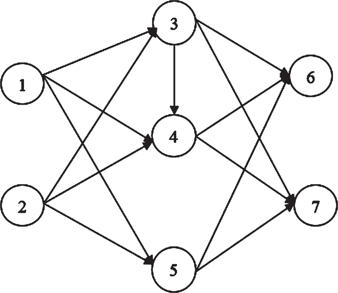
Example 1

This example is a network flow problem presented by Mahmoodirad et al. [18] consisting of sevenvertices and twelve arcs. In this example, the arc costs are represented by triangular fuzzy numbers. The details of this problem are shown in Fig. 1, Tables 1 and 2.

Fig. 1

Graph of Example 1.

Table 1

Fuzzy costs, fuzzy profit and crisp capacities of network arcs

Arc index	Tail node	Head node	Arc fuzzy cost (c_ij)	Arc fuzzy profit (d_ij)	Arc capacity
1	1	3	(5,40,90)	(20,30,50)	40
2	1	4	(4,45,115)	(30,40,60)	10
3	1	5	(5,57,116)	(60,80,100)	15
4	2	3	(10,40,85)	(5,70,80)	50
5	2	4	(10,50,120)	(80,90,100)	80
6	2	5	(13,60,164)	(50,60,70)	40
7	3	4	(2,10,25)	(90,110,120)	20
8	3	6	(8,50,145)	(70,80,100)	100
9	3	7	(2,35,105)	(10,30,40)	90
10	4	5	(3,10,40)	(20,30,40)	15
11	4	6	(8,40,115)	(40,60,80)	30
12	4	7	(5,25,56)	(80,90,110)	20
13	5	6	(5,30,75)	(20,40,60)	15
14	5	7	(2,10,40)	(40,50,60)	100

Table 2

Given capacities for the vertices of the Graph 1

b ₁	b ₂	b ₃	b ₄	b ₅	b ₆	b ₇
30	60	0	0	0	–20	–70

The same problem is solved by using the proposed Mehar approach, to obtain the following crisp non-dominated optimal solutions as

$\begin{matrix} x_{13} = 21.62, x_{15} = 8.378, x_{24} = 20, x_{25} = 40, \\ x_{36} = 20, x_{37} = 1.62, x_{47} = 20, x_{57} = 48.38, \\ x_{14} = x_{23} = x_{34} = x_{45} = x_{46} = x_{56} = 0 . \end{matrix}$

$\begin{matrix} x_{13} = 15.97, x_{15} = 14.03, x_{23} = 4.03, x_{24} = \\ 20, x_{25} = 35.97, x_{36} = 20, x_{45} = 15, x_{47} = 20, \\ x_{57} = 50, x_{14} = x_{34} = x_{37} = x_{46} = x_{56} = 0 . \end{matrix}$

$\begin{matrix} x_{13} = 15, x_{15} = 15, x_{23} = 15.09, x_{24} = 20, x_{25} \\ = 24.91, x_{36} = 20, x_{37} = 10.09, x_{45} = 15, x_{47} \\ = 20, x_{57} = 39.91, x_{14} = x_{34} = x_{46} = x_{56} = 0 . \end{matrix}$

and the corresponding non-dominated fuzzy optimal values of the fuzzy linear fractional minimal cost flow problem are

(0.0878, 0.5974, 1.892)

(0.0884, 0.5683, 1.2335)

(0. 0865, 0. 5742, 1. 982)

Example 2

This example is presented by Mahmoodirad et al. [18] to illustrate their proposed approach. In this example, the arc costs are represented by trapezoidal fuzzy numbers. The details of this problem are shown in Fig. 2, Tables 3 and 4.

Fig. 2

Graph of Example 2.

Table 3

Fuzzy costs, fuzzy profit and crisp capacities of network arcs

Arc index	Tail node	Head node	Arc fuzzy cost (c_ij)	Arc fuzzy profit (d_ij)	Lower bound	Upper bound
1	1	2	(80,10,150,182)	(30,40,50,80)	155	450
2	1	3	(242,250,300,320)	(20,25,35,40)	160	600
3	1	4	(21,25,75,91)	(10,20,30,40)	20	55
4	2	3	(137,150,200,225)	(18,22,34,46)	45	470
5	2	5	(90,100,400,434)	(12,13,14,17)	105	125
6	2	6	(155,180,220,265)	(30,40,50,80)	70	800
7	3	4	(105,125,225,261)	(20,25,35,40)	0	450
8	3	5	(95,100,200,225)	(30,40,50,80)	0	250
9	3	6	(98,110,240,260)	(30,45,55,80)	0	125
10	3	7	(270,300,400,470)	(28,42,74,96)	0	725
11	4	6	(78,120,280,310)	(10,20,30,40)	105	625
12	4	7	(140,150,200,222)	(10,20,30,40)	20	100
13	5	6	(0,0,0,0)	(10,12,13,14)	0	100
14	5	8	(l66,200,400,410)	(50,55,65,70)	0	135
15	5	9	(105,125,225,265)	(10,20,30,40)	0	625
16	6	7	(195.215.235.267)	(20,25,35,40)	15	175
17	6	8	(140,150,250,272)	(72,74,80,85)	70	160
18	6	9	(82,100,300.330)	(20.24,32,38)	80	190
19	6	10	(65.75,125,147)	(15,20,25,31)	30	750
20	7	9	(19,25,75.93)	(20.23.29.34)	0	230
21	7	10	(30,50,150,182)	(40,46,49,56)	0	220
22	8	9	(115,125,175,197)	(55,62,63,68)	30	110
23	8	11	(93,115,185.195)	(20,29,35,39)	25	120
24	8	12	(7,25,75,85)	(14,18,26,29)	0	215
25	9	10	(78.110,190,206)	(22,24,30.32)	5	200
26	9	11	(155,185.215,237)	(55,64,70,72)	40	140
27	9	12	(305,325,475.515)	(50,58,63.68)	80	190
28	9	13	(65,75,125,147)	(55,62,69,78)	5	340
29	10	12	(130,150,250,290)	(51,62,63.88)	0	165
30	10	13	(90.100,200,222)	(70,80,85,89)	0	220
31	11	12	(43,55,125,145)	(80,90.100,120)	15	340
32	11	14	(255,275,325,335)	(50,60.70,80)	0	110
33	12	13	(73,100,150,160)	(62,82.102,122)	25	215
34	12	14	(88,100,150,160)	(100,120,140.150)	20	135
35	13	14	190,200,300,350)	(25,45,65.90)	0	265

Table 4

Given capacities for the vertices of the Graph 2

b ₁	b ₂	b ₃	b ₄	b ₅	b ₆	b ₇	b ₈	b ₉	b ₁₀	b ₁₁	b ₁₂	b ₁₃	b ₁₄
350	100	–50	50	–50	100	–200	50	200	100	50	0	–100	–400

In this section, the same problem 2 is solved by the proposed Mehar approach.

Step 1: Using Step 1 of the proposed Mehar approach, the fuzzy optimal solution of the fuzzy linear fractional minimal cost flow problem can be obtained by solving its equivalent fuzzy linear fractional programming problem (P₂₁).

Problem (P₂₁)

$\min (\frac{u}{v})$

where,

$\begin{matrix} u = (80, 100, 150, 182) x_{12} + (242, 250, 300, 320) \\ x_{13} + (21, 25, 75, 91) x_{14} + (137, 150, 200, 225) x_{23} + \\ (90, 100, 400, 434) x_{25} + (155, 180, 220, 265) x_{26} + \\ (105, 125, 225, 261) x_{34} + (95, 100, 200, 225) x_{35} + \end{matrix}$

$\begin{matrix} (98, 110, 240, 260) x_{36} + (270, 300, 400, 470) x_{37} + \\ (78, 120, 280, 310) x_{46} + (140, 150, 200, 222) x_{47} + \\ (0, 0, 0, 0) x_{56} + (166, 200, 400, 410) x_{58} + \\ (105, 125, 225, 265) x_{59} + (195, 215, 235, 267) x_{67} + \\ (140, 150, 250, 272) x_{68} + (82, 100, 300, 330) x_{69} + \\ (65, 75, 125, 147) x_{610} + (19, 25, 75, 93) x_{79} + \\ (30, 50, 150, 182) x_{710} + (115, 125, 175, 197) x_{89} + \\ (93, 115, 185, 195) x_{811} + (7, 25, 75, 85) x_{812} + \\ (78, 110, 190, 206) x_{910} + (155, 185, 215, 237) x_{911} + \\ (305, 325, 475, 515) x_{912} + (65, 75, 125, 147) x_{913} + \end{matrix}$

$\begin{matrix} (130, 150, 250, 290) x_{1012} + (90, 100, 200, 222) x_{1013} + \\ (43, 55, 125, 145) x_{1112} + (255, 275, 325, 335) x_{1114} + \\ (78, 100, 150, 160) x_{1213} + (88, 100, 200, 224) x_{1214} + \\ (190, 200, 300, 350) x_{1314} \end{matrix}$

$\begin{matrix} v = (30, 40, 50, 80) x_{12} + (20, 25, 35, 40) x_{13} + \\ (10, 20, 30, 40) x_{14} + (18, 22, 34, 46) x_{23} + \\ (12, 13, 14, 17) x_{25} + (30, 40, 50, 80) x_{26} + \\ (20, 25, 35, 40) x_{34} + (30, 40, 50, 80) x_{35} + \\ (30, 45, 55, 80) x_{36} + (28, 42, 74, 96) x_{37} + \\ (10, 20, 30, 40) x_{46} + (10, 20, 30, 40) x_{47} + \\ (10, 12, 13, 14) x_{56} + (50, 55, 65, 70) x_{58} + \\ (10, 20, 30, 40) x_{59} + (20, 25, 35, 40) x_{67} + \\ (72, 74, 80, 85) x_{68} + (20, 24, 32, 38) x_{69} + \\ (15, 20, 25, 31) x_{610} + (20, 23, 29, 34) x_{79} + \end{matrix}$

$\begin{matrix} (40, 46, 49, 56) x_{710} + (55, 62, 63, 68) x_{89} + \\ (20, 29, 35, 39) x_{811} + (14, 18, 26, 29) x_{812} + \\ (22, 24, 30, 32) x_{910} + (55, 64, 70, 72) x_{911} + \\ (50, 58, 63, 68) x_{912} + (55, 62, 69, 78) x_{913} + \\ (51, 62, 63, 88) x_{1012} + (70, 80, 85, 89) x_{1013} + \\ (80, 90, 100, 120) x_{1112} + (50, 60, 70, 80) x_{1114} + \\ (62, 82, 102, 122) x_{1213} + (100, 120, 140, 150) x_{1214} + \\ (25, 45, 65, 90) x_{1314} \end{matrix}$

Subject to

x₁₂ + x₁₃ + x₁₄ = 350,

x₂₃ + x₂₅ + x₂₆ - x₁₂ = 100,

-x₁₃ - x₂₃ + x₃₄ + x₃₅ + x₃₆ + x₃₇ = -50,

x₄₆ + x₄₇ - x₁₄ - x₃₄ = 50,

-x₂₅ - x₃₅ + x₅₆ + x₅₈ + x₅₉ = -50,

x₆₇ + x₆₈ + x₆₉ + x₆₁₀ - x₂₆ - x₃₆ - x₄₆ - x₅₆ = 100,

-x₃₇ - x₄₇ - x₆₇ + x₇₉ + x₇₁₀ = -200,

x₈₉ + x₈₁₁ + x₈₁₂ - x₅₈ - x₆₈ = 50,.

x₉₁₀ + x₉₁₁ + x₉₁₂ + x₉₁₃ - x₅₉ - x₆₉ - x₇₉ - x₈₉ = 200,

-x₆₁₀ - x₇₁₀ - x₉₁₀ + x₁₀₁₂ + x₁₀₁₃ = -100,

x₁₁₁₂ + x₁₁₁₄ - x₈₁₁ - x₉₁₁ = 50,

x₁₂₁₃ + x₁₂₁₄ - x₈₁₂ - x₉₁₂ - x₁₀₁₂ - x₁₁₁₂ = 0,

-x₉₁₃ - x₁₀₁₃ - x₁₂₁₃ + x₁₃₁₄ = -100,

-x₁₁₁₄ - x₁₂₁₄ - x₁₃₁₄ = -400,

155 ⩽ x₁₂ ⩽ 450, 160 ⩽ x₁₃ ⩽ 600,

20 ⩽ x₁₄ ⩽ 550, 45 ⩽ x₂₃ ⩽ 470,

105 ⩽ x₂₅ ⩽ 125, 70 ⩽ x₂₆ ⩽ 800,

0 ⩽ x₃₄ ⩽ 450, 0 ⩽ x₃₅ ⩽ 250,

0 ⩽ x₃₆ ⩽ 125, 0 ⩽ x₃₇ ⩽ 725,

105 ⩽ x₄₆ ⩽ 625, 20 ⩽ x₄₇ ⩽ 100,

0 ⩽ x₅₆ ⩽ 100, 0 ⩽ x₅₈ ⩽ 135,

0 ⩽ x₅₉ ⩽ 625, 15 ⩽ x₆₇ ⩽ 175,

70 ⩽ x₆₈ ⩽ 160, 80 ⩽ x₆₉ ⩽ 190,

30 ⩽ x₆₁₀ ⩽ 750, 0 ⩽ x₇₉ ⩽ 230,

0 ⩽ x₇₁₀ ⩽ 220, 30 ⩽ x₈₉ ⩽ 110,

25 ⩽ x₈₁₁ ⩽ 120, 0 ⩽ x₈₁₂ ⩽ 215,

5 ⩽ x₉₁₀ ⩽ 200, 40 ⩽ x₉₁₁ ⩽ 140,

80 ⩽ x₉₁₂ ⩽ 190, 5 ⩽ x₉₁₃ ⩽ 340,

0 ⩽ x₁₀₁₂ ⩽ 165, 0 ⩽ x₁₀₁₃ ⩽ 220,

15 ⩽ x₁₁₁₂ ⩽ 340, 0 ⩽ x₁₁₁₄ ⩽ 110,

25 ⩽ x₁₂₁₃ ⩽ 215, 20 ⩽ x₁₂₁₄ ⩽ 135,

0 ⩽ x₁₃₁₄ ⩽ 265.

Step 2: Using Step 2 of the proposed Mehar approach, the fuzzy linear fractional programming problem (P₂₁) can be transformed into its equivalent fuzzy linear fractional programming problem (P₂₂).

Problem (P₂₂)

$min (\frac{u_{1}, u_{2}, u_{3}, u_{4}}{v_{1}, v_{2}, v_{3}, v_{4}})$

where,

$\begin{matrix} u_{1} = 80 x_{12} + 242 x_{1} 3 + 21 x_{14} + 137 x_{23} + 90 x_{25} + \\ 155 x_{26} + 105 x_{34} + 95 x_{35} + 98 x_{36} + 270 x_{37} + \\ 78 x_{46} + 140 x_{47} + 166 x_{58} + 105 x_{59} + 195 x_{67} + \\ 140 x_{68} + 82 x_{69} + 65 x_{610} + 19 x_{79} + 30 x_{710} + \\ 115 x_{89} + 93 x_{811} + 7 x_{812} + 78 x_{910} + 155 x_{911} + \\ 305 x_{912} + 65 x_{913} + 130 x_{1012} + 90 x_{1013} + \\ 43 x_{1112} + 255 x_{1114} + 78 x_{1213} + 88 x_{1214} + 190 x_{1314}, \end{matrix}$

$\begin{matrix} u_{2} = 100 x_{12} + 250 x_{13} + 25 x_{14} + 150 x_{23} + 100 x_{25} + \\ 180 x_{26} + 125 x_{34} + 100 x_{35} + 110 x_{36} + 300 x_{37} + \\ 120 x_{46} + 150 x_{47} + 200 x_{58} + 125 x_{59} + 215 x_{67} + \\ 150 x_{68} + 100 x_{69} + 75 x_{610} + 25 x_{79} + 50 x_{710} + \\ 125 x_{89} + 115 x_{811} + 25 x_{812} + 110 x_{910} + 185 x_{911} + \\ 325 x_{912} + 75 x_{913} + 150 x_{1012} + 100 x_{1013} + 55 x_{1112} + \\ 275 x_{1114} + 100 x_{1213} + 100 x_{1214} + 200 x_{1314}, \end{matrix}$

$\begin{matrix} u_{3} = 150 x_{12} + 300 x_{13} + 75 x_{14} + 200 x_{23} + 400 x_{25} + \\ 220 x_{26} + 225 x_{34} + 200 x_{35} + 240 x_{36} + 400 x_{37} + \\ 280 x_{46} + 200 x_{47} + 400 x_{58} + 225 x_{59} + 235 x_{67} + \\ 250 x_{68} + 300 x_{69} + 125 x_{610} + 75 x_{79} + 150 x_{710} + \\ 175 x_{89} + 185 x_{811} + 75 x_{812} + 190 x_{910} + 215 x_{911} + \\ 475 x_{912} + 125 x_{913} + 250 x_{1012} + 200 x_{1013} + \\ 125 x_{1112} + 325 x_{1114} + 150 x_{1213} + 200 x_{1214} + 300 x_{1314}, \end{matrix}$

$\begin{matrix} u_{4} = 182 x_{12} + 320 x_{13} + 91 x_{14} + 225 x_{23} + 434 x_{25} + \\ 265 x_{26} + 261 x_{34} + 225 x_{35} + 260 x_{36} + 470 x_{37} + \\ 310 x_{46} + 222 x_{47} + 410 x_{58} + 265 x_{59} + 267 x_{67} + \\ 272 x_{68} + 330 x_{69} + 147 x_{610} + 93 x_{79} + 182 x_{710} + \\ 197 x_{89} + 195 x_{811} + 85 x_{812} + 206 x_{910} + 237 x_{911} + \\ 515 x_{912} + 147 x_{913} + 290 x_{1012} + 222 x_{1013} + \\ 145 x_{1112} + 335 x_{1114} + 160 x_{1213} + 224 x_{1214} + \\ 350 x_{1314}, \end{matrix}$

$\begin{matrix} v_{1} = 30 x_{12} + 20 x_{13} + 10 x_{14} + 18 x_{23} + 12 x_{25} + \\ 30 x_{26} + 20 x_{34} + 30 x_{35} + 30 x_{36} + 28 x_{37} + 10 x_{46} + \\ 10 x_{47} + 10 x_{56} + 50 x_{58} + 10 x_{59} + 20 x_{67} + 72 x_{68} + \end{matrix}$

$\begin{matrix} 20 x_{69} + 15 x_{610} + 20 x_{79} + 40 x_{710} + 55 x_{89} + 20 x_{811} + \\ 14 x_{812} + 22 x_{910} + 55 x_{911} + 50 x_{912} + 55 x_{913} + \\ 51 x_{1012} + 70 x_{1013} + 80 x_{1112} + 50 x_{1114} + 62 x_{1213} + \\ 100 x_{1214} + 25 x_{1314}, \end{matrix}$

$\begin{matrix} v_{2} = 40 x_{12} + 25 x_{13} + 20 x_{14} + 22 x_{23} + 13 x_{25} + \\ 40 x_{26} + 25 x_{34} + 40 x_{35} + 45 x_{36} + 42 x_{37} + 20 x_{46} + \\ 20 x_{47} + 12 x_{56} + 55 x_{58} + 20 x_{59} + 25 x_{67} + 74 x_{68} + \\ 24 x_{69} + 20 x_{610} + 23 x_{79} + 46 x_{710} + 62 x_{89} + 29 x_{811} + \\ 18 x_{812} + 24 x_{910} + 64 x_{911} + 58 x_{912} + 62 x_{913} + \\ 62 x_{1012} + 80 x_{1013} + 90 x_{1112} + 60 x_{1114} + 82 x_{1213} + \\ 120 x_{1214} + 45 x_{1314}, \end{matrix}$

$\begin{matrix} v_{3} = 50 x_{12} + 35 x_{13} + 30 x_{14} + 34 x_{23} + 14 x_{25} + \\ 50 x_{26} + 35 x_{34} + 50 x_{35} + 55 x_{36} + 74 x_{37} + 30 x_{46} + \\ 30 x_{47} + 13 x_{56} + 65 x_{58} + 30 x_{59} + 35 x_{67} + 80 x_{68} + \\ 32 x_{69} + 25 x_{610} + 29 x_{79} + 49 x_{710} + 63 x_{89} + \\ 35 x_{811} + 26 x_{812} + 30 x_{910} + 70 x_{911} + 63 x_{912} + \\ 69 x_{913} + 63 x_{1012} + 85 x_{1013} + 100 x_{1112} + \\ 70 x_{1114} + 102 x_{1213} + 140 x_{1214} + 65 x_{1314}, \end{matrix}$

$\begin{matrix} v_{4} = 80 x_{12} + 40 x_{13} + 40 x_{14} + 46 x_{23} + 17 x_{25} + \\ 80 x_{26} + 40 x_{34} + 80 x_{35} + 80 x_{36} + 96 x_{37} + 40 x_{46} + \\ 40 x_{47} + 14 x_{56} + 70 x_{58} + 40 x_{59} + 40 x_{67} + 85 x_{68} + \\ 38 x_{69} + 31 x_{610} + 34 x_{79} + 56 x_{710} + 68 x_{89} + \\ 39 x_{811} + 29 x_{812} + 32 x_{910} + 72 x_{911} + 68 x_{912} + \\ 78 x_{913} + 88 x_{1012} + 89 x_{1013} + 120 x_{1112} + \\ 80 x_{1114} + 122 x_{1213} + 150 x_{1214} + 90 x_{1314} \end{matrix}$

Subject to

Constraints of the problem (P₂₁).

Step 3: Using Step 3 of the proposed Mehar approach, the fuzzy linear fractional programming problem (P₂₂) can be transformed into its equivalent crisp multi-objective linear fractional programming problem (P₂₃).

Problem (P₂₃)

$min (\frac{u_{1}}{v_{4}})$

$min (\frac{u_{2}}{v_{3}})$

$min (\frac{u_{3}}{v_{2}})$

$min (\frac{u_{4}}{v_{1}})$

Subject to

Constraints of the problem (P₂₁).

Step 4: Using Step 4 of the proposed Mehar approach, there is a need to apply lexicographic approach [19] to solve the crisp multi-objective linear fractional programming problem (P₂₃).

Using the lexicographic approach [19], the obtained crisp non-dominated optimal solutions are

$\begin{matrix} x_{12} = 155, x_{13} = 160, x_{14} = 35, x_{23} = 45, x_{25} = \\ 105, x_{26} = 105, x_{34} = 45, x_{35} = 45, x_{36} = 65, x_{37} = \\ 0, x_{46} = 105, x_{47} = 25, x_{56} = 100, x_{58} = 0, x_{59} = \\ 0, x_{67} = 175, x_{68} = 140, x_{69} = 80, x_{610} = 80, x_{79} = \\ 0, x_{710} = 0, x_{89} = 110, x_{811} = 80, x_{812} = 0, x_{910} = \\ 20, x_{911} = 140, x_{912} = 80, x_{913} = 150, x_{1} 012 = \\ 0, x_{1013} = 0, x_{1112} = 270, x_{1114} = 0, x_{1213} = \\ 215, x_{1214} = 135, x_{1314} = 265 . \end{matrix}$

$\begin{matrix} x_{12} = 155, x_{13} = 160, x_{14} = 35, x_{23} = 71, x_{25} = \\ 105, x_{26} = 79, x_{34} = 45, x_{35} = 45, x_{36} = 91, x_{37} = \\ 0, x_{46} = 105, x_{47} = 25, x_{56} = 100, x_{58} = 0, x_{59} = \\ 0, x_{67} = 175, x_{68} = 140, x_{69} = 80, x_{610} = 80, x_{79} = \\ 0, x_{710} = 0, x_{89} = 110, x_{811} = 80, x_{812} = 0, x_{910} = \\ 20, x_{911} = 140, x_{912} = 80, x_{913} = 150, x_{1012} = \\ 0, x_{1013} = 0, x_{1112} = 270, x_{1114} = 0, x_{1213} = \\ 215, x_{1214} = 135, x_{1314} = 265 . \end{matrix}$

$\begin{matrix} x_{12} = 155, x_{13} = 160, x_{14} = 35, x_{23} = 45, x_{25} = \\ 105, x_{26} = 105, x_{34} = 40, x_{35} = 45, x_{36} = 65, x_{37} = \\ 5, x_{46} = 105, x_{47} = 20, x_{56} = 100, x_{58} = 0, x_{59} = \\ 0, x_{67} = 175, x_{68} = 159, x_{69} = 80, x_{610} = 61, x_{79} = \\ 0, x_{710} = 0, x_{89} = 110, x_{811} = 99, x_{812} = 0, x_{910} = \\ 39, x_{911} = 140, x_{912} = 80, x_{913} = 131, x_{1012} = \\ 0, x_{1013} = 0, x_{1112} = 270, x_{1114} = 19, x_{1213} = \\ 215, x_{1214} = 135, x_{1314} = 246 . \end{matrix}$

$\begin{matrix} x_{12} = 155, x_{13} = 160, x_{14} = 35, x_{23} = 45, x_{25} = \\ 105, x_{26} = 105, x_{34} = 40, x_{35} = 45, x_{36} = 65, x_{37} = \\ 5, x_{46} = 105, x_{47} = 20, x_{56} = 100, x_{58} = 0, x_{59} = \\ 0, x_{67} = 175, x_{68} = 134, x_{69} = 80, x_{610} = 86, x_{79} = \\ 0, x_{710} = 0, x_{89} = 104, x_{811} = 80, x_{812} = 0, x_{910} = \\ 14, x_{911} = 140, x_{912} = 80, x_{913} = 150, x_{1012} = \\ 0, x_{1013} = 0, x_{1112} = 270, x_{1114} = 0, x_{1213} = \\ 215, x_{1214} = 135, x_{1314} = 265 . \end{matrix}$

$\begin{matrix} x_{12} = 155, x_{13} = 160, x_{14} = 35, x_{23} = 80, x_{25} = \\ 105, x_{26} = 70, x_{34} = 45, x_{35} = 45, x_{36} = 100, x_{37} = \\ 0, x_{46} = 105, x_{47} = 25, x_{56} = 100, x_{58} = 0, x_{59} = \\ 0, x_{67} = 175, x_{68} = 160, x_{69} = 80, x_{610} = 60, x_{79} = \\ 0, x_{710} = 0, x_{89} = 80, x_{811} = 120, x_{812} = 10, x_{910} = \\ 40, x_{911} = 90, x_{912} = 80, x_{913} = 150, x_{1012} = \end{matrix}$

$\begin{matrix} 0, x_{1013} = 0, x_{1112} = 260, x_{1114} = 0, x_{1213} = \\ 215, x_{1214} = 135, x_{1314} = 265 . \end{matrix}$

$\begin{matrix} x_{12} = 155, x_{13} = 160, x_{14} = 35, x_{23} = 67, x_{25} = \\ 105, x_{26} = 83, x_{34} = 45, x_{35} = 45, x_{36} = 87, x_{37} = \\ 0, x_{46} = 105, x_{47} = 25, x_{56} = 100, x_{58} = 0, x_{59} = \\ 0, x_{67} = 175, x_{68} = 160, x_{69} = 80, x_{610} = 60, x_{79} = \\ 0, x_{710} = 0, x_{89} = 90, x_{811} = 120, x_{812} = 0, x_{910} = \\ 40, x_{911} = 100, x_{912} = 80, x_{913} = 150, x_{1012} = \\ 0, x_{1013} = 0, x_{1112} = 270, x_{1114} = 0, x_{1213} = \\ 215, x_{1214} = 135, x_{1314} = 265 . \end{matrix}$

$\begin{matrix} x_{12} = 155, x_{13} = 160, x_{14} = 35, x_{23} = 73, x_{25} = \\ 105, x_{26} = 77, x_{34} = 45, x_{35} = 45, x_{36} = 93, x_{37} = \\ 0, x_{46} = 105, x_{47} = 25, x_{56} = 100, x_{58} = 0, x_{59} = \\ 0, x_{67} = 175, x_{68} = 160, x_{69} = 80, x_{610} = 60, x_{79} = \\ 0, x_{710} = 0, x_{89} = 90, x_{811} = 120, x_{812} = 0, x_{910} = \\ 40, x_{911} = 100, x_{912} = 80, x_{913} = 150, x_{1012} = \\ 0, x_{1013} = 0, x_{1112} = 270, x_{1114} = 0, x_{1213} = \\ 215, x_{1214} = 135, x_{1314} = 265 . \end{matrix}$

$\begin{matrix} x_{12} = 155, x_{13} = 160, x_{14} = 35, x_{23} = 45, x_{25} = \\ 105, x_{26} = 105, x_{34} = 40, x_{35} = 45, x_{36} = 65, x_{37} = \\ 5, x_{46} = 105, x_{47} = 20, x_{56} = 100, x_{58} = 0, x_{59} = \\ 0, x_{67} = 175, x_{68} = 160, x_{69} = 80, x_{610} = 60, x_{79} = \\ 0, x_{710} = 0, x_{89} = 110, x_{811} = 100, x_{812} = 0, x_{910} = \\ 40, x_{911} = 128, x_{912} = 80, x_{913} = 142, x_{1012} = \\ 0, x_{1013} = 0, x_{1112} = 270, x_{1114} = 8, x_{1213} = \\ 215, x_{1214} = 135, x_{1314} = 257 . \end{matrix}$

$\begin{matrix} x_{12} = 155, x_{13} = 160, x_{14} = 35, x_{23} = 45, x_{25} = \\ 105, x_{26} = 105, x_{34} = 40, x_{35} = 45, x_{36} = 65, x_{37} = \\ 5, x_{46} = 105, x_{47} = 20, x_{56} = 100, x_{58} = 0, x_{59} = \\ 0, x_{67} = 175, x_{68} = 125, x_{69} = 80, x_{610} = 95, x_{79} = \\ 0, x_{710} = 0, x_{89} = 83, x_{811} = 92, x_{812} = 0, x_{910} = \\ 5, x_{911} = 128, x_{912} = 80, x_{913} = 150, x_{1012} = \\ 0, x_{1013} = 0, x_{1112} = 270, x_{1114} = 0, x_{1213} = \\ 215, x_{1214} = 135, x_{1314} = 265 . \end{matrix}$

$\begin{matrix} 30, x_{911} = 140, x_{912} = 80, x_{913} = 140, x_{1012} = \\ 0, x_{1013} = 0, x_{1112} = 270, x_{1114} = 10, x_{1213} = \\ 215, x_{1214} = 135, x_{1314} = 255 . \end{matrix}$

$\begin{matrix} x_{12} = 155, x_{13} = 160, x_{14} = 35, x_{23} = 73, x_{25} = \\ 105, x_{26} = 76, x_{34} = 45, x_{35} = 45, x_{36} = 93, x_{37} = \\ 0, x_{46} = 105, x_{47} = 25, x_{56} = 100, x_{58} = 0, x_{59} = \\ 0, x_{67} = 175, x_{68} = 160, x_{69} = 80, x_{610} = 60, x_{79} = \\ 0, x_{710} = 0, x_{89} = 90, x_{811} = 120, x_{812} = 0, x_{910} = \\ 40, x_{911} = 100, x_{912} = 80, x_{913} = 150, x_{1012} = \\ 0, x_{1013} = 0, x_{1112} = 270, x_{1114} = 0, x_{1213} = \\ 215, x_{1214} = 135, x_{1314} = 265 . \end{matrix}$

$\begin{matrix} x_{12} = 155, x_{13} = 160, x_{14} = 35, x_{23} = 45, x_{25} = \\ 105, x_{26} = 105, x_{34} = 40, x_{35} = 45, x_{36} = 65, x_{37} = \\ 5, x_{46} = 105, x_{47} = 20, x_{56} = 100, x_{58} = 0, x_{59} = \\ 0, x_{67} = 175, x_{68} = 160, x_{69} = 80, x_{610} = 60, x_{79} = \\ 0, x_{710} = 0 {, x}_{89} = 106, x_{811} = 104, x_{812} = 0, x_{910} = \\ 40, x_{911} = 116, x_{912} = 80, x_{913} = 150, x_{1012} = \\ 0, x_{1013} = 0, x_{1112} = 270, x_{1114} = 0, x_{1213} = \\ 215, x_{1214} = 135, x_{1314} = 265 . \end{matrix}$

$\begin{matrix} x_{12} = 155, x_{13} = 160, x_{14} = 35, x_{23} = 45, x_{25} = \\ 105, x_{26} = 105, x_{34} = 40, x_{35} = 45, x_{36} = 65, x_{37} = \\ 5, x_{46} = 105, x_{47} = 20, x_{56} = 100, x_{58} = 0, x_{59} = \\ 0, x_{67} = 175, x_{68} = 125, x_{69} = 80, x_{610} = 95, x_{79} = \\ 0, x_{710} = 0, x_{89} = 94, x_{811} = 81, x_{812} = 0, x_{910} = \\ 5, x_{911} = 139, x_{912} = 80, x_{913} = 150, x_{1012} = \\ 0, x_{1013} = 0, x_{1112} = 270, x_{1114} = 0, x_{1213} = \\ 215, x_{1214} = 135, x_{1314} = 265 . \end{matrix}$

$\begin{matrix} 0, x_{710} = 0, x_{89} = 100, x_{811} = 80, x_{812} = 0, x_{910} = \\ 10, x_{911} = 140, x_{912} = 80, x_{913} = 150, x_{1012} = \\ 0, x_{1013} = 0, x_{1112} = 270, x_{1114} = 0, x_{1213} = \\ 215, x_{1214} = 135, x_{1314} = 265 . \end{matrix}$

$\begin{matrix} x_{12} = 155, x_{13} = 160, x_{14} = 35, x_{23} = 45, x_{25} = \\ 105, x_{26} = 105, x_{34} = 45, x_{35} = 45, x_{36} = 65, x_{37} = \\ 0, x_{46} = 105, x_{47} = 25, x_{56} = 100, x_{58} = 0, x_{59} = \\ 0, x_{67} = 175, x_{68} = 149, x_{69} = 80, x_{610} = 71, x_{79} = \\ 0, x_{710} = 0, x_{89} = 79, x_{811} = 120, x_{812} = 0, x_{910} = \\ 29, x_{911} = 100, x_{912} = 80, x_{913} = 150, x_{1012} = \\ 0, x_{1013} = 0, x_{1112} = 270, x_{1114} = 0, x_{1213} = \\ 215, x_{1214} = 135, x_{1314} = 265 . \end{matrix}$

$\begin{matrix} x_{12} = 155, x_{13} = 160, x_{14} = 35, x_{23} = 45, x_{25} = \\ 105, x_{26} = 105, x_{34} = 45, x_{35} = 45, x_{36} = 65, x_{37} = \\ 0, x_{46} = 105, x_{47} = 25, x_{56} = 100, x_{58} = 0, x_{59} = \\ 0, x_{67} = 175, x_{68} = 127, x_{69} = 80, x_{610} = 93, x_{79} = \\ 0, x_{710} = 0, x_{89} = 57, x_{811} = 120, x_{812} = 0, x_{910} = \\ 7, x_{911} = 100, x_{912} = 80, x_{913} = 150, x_{1012} = \\ 0, x_{1013} = 0, x_{1112} = 270, x_{1114} = 0, x_{1213} = \\ 215, x_{1214} = 135, x_{1314} = 265 . \end{matrix}$

Step 5: Using the non-dominated optimal solutions, the non-dominated fuzzy optimal values of the fuzzy linear fractional programming problem (P₂₁) are

(1.59989, 2.19416, 4.22094, 5.86549)

(1.60066, 2.19335, 4.23949, 5.89031)

(1.62685, 2.21313, 3.78379, 5.85903)

(1.59927, 2.12159, 4.22464, 5.87849)

(1.60305, 2.20242, 4.31577, 6)

(1.63354, 2.19633, 4.06151, 6.05462)

(1.59987, 2.19613, 4.28278, 5.94617)

(1.60713, 2.20259, 4.23675, 5.85609)

(1.59747, 2.19696, 4.24794, 5.90112)

(1.60853, 2.14845, 4.23041, 5.86204)

(1.59974, 2.19574, 4.04527, 5.40142)

(1.60155, 2.23370, 4.45201, 6.23112)

(1.60016, 2.19535, 4.38487, 5.20228)

(1.59828, 2.19569, 4.37985, 5.20228)

(1.59886, 2.19515, 4.22741, 5.25513)

(1.59918, 2.12588, 4.26662, 5.21362)

(1.59690, 2.12647, 4.28766, 5.24240)

8 Conclusions

On the basis of the present study, it can be easily concluded that some mathematical incorrect assumptions are considered in Mahmoodirad et al.’s approach [18]. Hence, it is inappropriate to use Mahmoodirad et al.’s approach [18]. Also, it can be concluded that the proposed Mehar approach can be used to solve the existing fuzzy linear fractional minimal cost flow problems [18]. Furthermore, it is pertinent to mention that the proposed Mehar approach, in its present form, cannot be used to solve such linear fractional minimal cost flow problems in which all the parameters are either represented by triangular fuzzy numbers or trapezoidal fuzzy numbers. In future, to overcome this limitation, one may generalize the proposed Mehar approach.

Footnotes

Acknowledgments

The authors would like to thank the Editor-in-Chief, the handling Editor and anonymous reviewers for their insightful comments and suggestions.

References

Ahuja

R.K.

, Magnanti

T.L.

, Orlin

J.B.

, Network Flows: Theory, algorithms and applications, Prentice-Hall, Englewood Cliffs, NJ, 1993.

Sherali

H.D.

, On a fractional minimal cost flow problem on networks, Optimization Letters 6(8) (2012), 1945–1949.

Fakhri

, Ghatee

, Fractional multi-commodity flow problem: duality and optimality conditions, Applied Mathematical Modelling 38(7-8) (2014), 2151–2162.

Zadeh

L.A.

, Fuzzy sets, Information and Control 8(3) (1965), 338–353.

Kaur

, Kumar

, An introduction to fuzzy linear programming problems, Springer International Publishing, Switzerland, 2016.

Chakraborty

, Gupta

, Fuzzy mathematical programming for multi objective linear fractional programming problem, Fuzzy Sets and Systems 125(3) (2002), 335–342.

Pop

, Stancu-Minasian

I.M.

, A method of solving fully fuzzified linear fractional programming problems, Journal of Applied Mathematics and Computing 27(1) (2008), 227–242.

Stanojevic

, Stancu-Minasian

I.M.

, Evaluating fuzzy inequalities and solving fully fuzzified linear fractional programs, Yugoslav Journal of Operations Reserach 22(1) (2012), 41–50.

Stanojević

, Stanojević

, Comment on “Fuzzy mathematical programming for multi objective linear fractional programming problem”, Fuzzy Sets and Systems 246 (2014), 156–159.

10.

Veeramani

, Sumathi

, Fuzzy mathematical programming approach for solving fuzzy linear fractional programming problem, RAIRO-Operations research 48(1) (2014), 109–122.

11.

Veeramani

, Sumathi

, Solving the linear fractional programming problem in a fuzzy environment: Numerical approach, Applied Mathematical Modelling 40(11-12) (2016), 6148–6164.

12.

Das

S.K.

, Mandal

, Edalatpanah

S.A.

, A new approach for solving fully fuzzy linear fractional programming problems using the multi-objective linear programming, RAIRO-Operations Research 51(1) (2017), 285–297.

13.

Arya

, Singh

, Kumari

, Obaidat

M.S.

, An approach for solving fully fuzzy multi-objective linear fractional optimization problems, Soft Computing 24(12) (2020), 9105–9119.

14.

Das

S.K.

, Edalatpanah

S.A.

, Mandal

, Application of linear fractional programming problem with fuzzy nature in industry sector, Filomat 34(15) (2020), 5073–5084.

15.

Das

S.K.

, Edalatpanah

S.A.

, Mandal

, Development of unrestricted fuzzy linear fractional programming problems applied in real case, Fuzzy Information and Engineering 13(2) (2021), 184–195.

16.

Kaur

, Kacprzyk

, Kumar

, Fuzzy transportation and transshipment problems, Springer Nature Switzerland AG, Switzerland, 2020.

17.

Verma

, Kumar

, Fuzzy solution concepts for non-cooperative games: Interval, fuzzy and intuitionistic fuzzy payoffs, Springer Nature Switzerland AG, Switzerland, 2020.

18.

Mahmoodirad

, Niroomand

, Mirzaei

, Shoja

, Fuzzy fractional minimal cost flow problem, International Journal of Fuzzy Systems 20(1) (2018), 174–186.

19.

Bajalinov

E.B.

, Linear-fractional programming: Theory, methods, applications and software, Kluwer Academic Publishers, Boston, 2003.

20.

Bector

C.R.

, Chandra

, Fuzzy mathematical programming and fuzzy matrix games, Springer Berlin Heidelberg, New York, 2005.

21.

Zimmermann

H.J.

, Fuzzy set theory and its applications, Kluwer Academic Publishers, Boston, 2001.