A data-driven degradation prognostics approach for rolling element bearings

Abstract

Degradation prognostic plays a crucial role in increasing the efficiency of health management for rolling element bearings (REBs). In this paper, a novel four-step data-driven degradation prognostics approach is proposed for REBs. In the first step, a series of degradation features are extracted by analyzing the vibration signals of REBs in time domain, frequency domain and time-frequency domain. In the second step, three indicators are utilized to select the sensitive features. In the third step, different health state labels are automatically assigned for health state estimation, where the influence of uncertain initial condition is eliminated. In the last step, a multivariate health state estimation model and a multivariate multistep degradation trend prediction model are combined to estimate the residence time in different health status and remaining useful life (RUL) of REBs. Verification results using the XJTU-SY datasets validate the effectiveness of the proposed method and show a more accurate prognostics results compared with the existing major approaches.

Keywords

Degradation prognostic rolling element bearings (REBs)health state estimation remaining useful life (RUL)

1 Introduction

As an incredible critical component of rotating machinery, rolling element bearings (REBs) are widely used in aerospace equipment, transportation tools and wind power generation equipment [1]. The wear of the bearings can cause damage to the mechanical equipment, which may lead to serious accidents. Degradation prognostic is the key part of health management in condition monitoring (CM), remaining useful life (RUL) prediction, and operation optimization [2]. The goal of degradation prognostic is to avoid catastrophic failure, improve the stability, and extend the life-span of equipment. Therefore, developing the degradation prognostics techniques of REBs have become an urgent need.

Generally, the degradation prognostics mainly include two categories: 1) model-based method and 2) data-driven method [3]. The model-based method builds a corresponding model according to the physical structure, operating principle and degradation mechanism of the system [4 –6]. This method can clearly describe the degradation process of the system, which leads to a good prediction performance for the system with simple physical structure and clear degradation mechanism. However, in practical engineering, the operating conditions of the equipment are extremely complex and dynamic. Therefore, the general physical model cannot match the actual situation perfectly, which may affect the prognostics results [7]. The data-driven method establishes a degradation prognostic model based on the historical CM data collected by the sensors [8 –12]. The health status and RUL of the equipment can be predicted by analyzing the degradation trend of the features. This method does not require the knowledge about the physical structure of the system, and thus, it is very suitable for the complex system like rotating machinery.

Data-driven prognostics methods can be further classified into three major branches [13]: 1) direct prognostics modeling; 2) univariate prognostics modeling and 3) multivariate prognostics modeling. Direct prognostics modeling learns the relation between the current observed degradation trend and the RUL by using the historical CM data, and then the degradation prognostic model can be established according to the relationship [14]. Finally, it can match the online observed data with the prognostic model to calculate the corresponding RUL of the equipment, as shown in Fig. 1(a). This model does not need to set the failure threshold (FT). However, it needs to train abundant CM data in order to obtain an accurate prediction model, and thus, it is difficult to realize in engineering because of its high complexity and large calculation.

Fig. 1

Classification of data-driven degradation prediction methods.(a) Direct prognostics modeling. (b) Univariate prognostics modeling. (c) Multivariate prognostics modeling.

Univariate prognostics modeling obtains the RUL by constructing an one-dimensional health index (HI) [15, 16]. The prognostics is completed when the HI reaches the predefined FT, as shown in Fig. 1(b). The advantage of this method is that it doesn’t need to know the whole life data of the equipment. However, it is very difficult to get a precise and reasonable HI [17].

In multivariate prognostics modeling, clustering analysis and classification methods are usually adopted for dividing the historical degradation data into several subsets, which represent the different health status [18]. Regression analysis or time-series analysis can be used to build multivariate degradation model for calculating the time interval between the current state and the failure state, as shown in Fig. 1(c). This model has two major advantages: 1) Comparing with the direct prognostics modeling, it does not need much training and can improve the computational efficiency. 2) Comparing with the univariate prognostics modeling, multivariate CM data can provide more comprehensive degradation information, making the prediction results more accurate.

Multivariate prognostics modeling is initially proposed in [19], and the implementation details of this method are given in [20]. In recent years, it has gradually become an emerging technique in prognostics field [21 –25]. However, the existing approaches rarely take into account the residence time of different health states and uncertainty of the initial condition, and they often need to preset a FT. In reference [21], degradation process of the REBs is divided into health status and failure status according to a preset FT. Then, Kalman filter (KF) is used to estimate the RUL of REBs. However, this method only divides the degradation process into two discrete states, which is hard to formulate a flexible maintenance strategy. At the same time, the preset FT also reduces the accuracy of the prognostics results. As the further improvement in [22], the Markov classifier is implemented to divide the continuous degradation process of the engine into four different health states. However, this method ignores uncertainty of initial conditions and cannot calculate the residence time of different health states. In reference [23, 24] and [25], deep neural network (DNN), support vector machine (SVM) and hidden Markov model (HMM) are, respectively, implemented to construct health states classifiers. However, the implementation of these methods both need a preset FT and the influence of uncertain initial condition is also ignored. Therefore, a new degradation prognostic approach is proposed, which takes into account initial condition uncertainty and does not need to preset a FT. Meanwhile, the residence time in different health states of the REBs can be calculated, which facilitates to formulate the maintenance strategy more flexibly.

In this paper, a novel four-step data-driven degradation prognostic approach is proposed, consisting of degradation feature extraction (step 1), degradation feature selection (step 2), offline health state assessment and degradation trend prediction modeling (step 3), and online RUL prognostics (step 4). Firstly, a series of degradation features are extracted by analyzing the vibration signals of REBs in time domain, frequency domain and time-frequency domain. Then, three indicators regarding the monotonicity, correlation and robustness are utilized to select the sensitive features. On this basis, the offline health state estimation model and degradation trend prediction model are established respectively. Finally, the above two models are combined to estimate the residence time in different health states and the RUL of REBs. The main contributions of this paper are summarized as follows:

1) A variety of degradation features are extracted by comprehensive analyses of time domain, frequency domain and time-frequency domain.

2) Different health state labels can be assigned automatically. It also eliminates the influence of uncertain initial condition on the prediction results.

3) The degradation prognostic is finished when the two termination conditions are both met instead of predefining an unreasonable FT. Therefore, the proposed approach can obtain a higher prediction accuracy.

4) With a health state estimation model and a degradation trend prediction model, the residence time in different health states of REBs can be estimated, which facilitates to formulate the maintenance strategy more flexibly.

The remainder of this paper is organized as follows. Section II shows the framework of the proposed data-driven degradation prognostics approach. Section III provides details of the four-step degradation prognostics approach. Section IV presents the verification results by using the data set from the accelerated degradation testing of REBs. Finally, the conclusion is drawn in Section V.

2 Framework of proposed data-driven degradation prognostics approach

Fig. 2 shows the framework of the proposed data-driven degradation prediction strategy for REBs, and the two initial hypotheses of the proposed method are as follows.

Fig. 2

Framework of the data-driven degradation prognostics strategy.

Hypothesis 1: The degradation process of REBs is divided into four health states: health state, mild degradation state, moderate degradation state and near failure state. Meanwhile, the initial condition of each REB is assumed as different.

Hypothesis 2: The degradation prognostic will be finished when the two termination conditions are both met: (1) The output of gate recurrent unit (GRU) network is evaluated as the last state. (2) Degradation trend of one feature is constant.

On these bases, this paper proposes a novel degradation prognostic strategy, which includes the following four main steps.

1) Degradation feature extraction. In the first step, multiple degradation features are extracted from the raw vibration signals, consisting of statistical features and nonlinear features. The statistical features are calculated by time domain and frequency domain analyses. Complete ensemble empirical mode decomposition with adaptive noise (CEEMDAN) and Hilbert-Huang transform (HHT) time-frequency analysis are used to calculate the nonlinear features.

2) Degradation feature selection. In the second step, the optimal features are picked out by analyzing the three indicators on correlation, monotonicity and robustness of the original degradation features.

3) Offline health state assessment and degradation trend prediction modeling. In the third step, firstly, the health state labels are assigned to the unfolded 2-D optimal feature matrix automatically by the density peak clustering (DPC) algorithm, and then the features with completed labels are input into the multivariate deep forest (DF) classifier to train for getting the offline health state assessment model. Secondly, all univariate GRU networks of the selected features are combined to obtain the multivariate multistep GRU network for degradation trend prediction.

4) Online RUL prognostics. In the final step, the GRU based degradation trend prediction model is utilized to predict the feature value at the next moment, and then the health state assessment model is used to estimate the health state of the predicted value. The above two models are combined to perform multistep prediction until the termination conditions of REBs are met. Therefore, the residence time in different health status and the RUL can be obtained.

3 Four-step degradation prognostics approach

3.1 Step 1: Degradation feature extraction

First of all, moving average method and data standardization technology are performed on the raw vibration signals to eliminate the influence of noise and dimension. Then, the following two types of features are extracted from the preprocessed vibration signals respectively.

3.1.1 Statistical features extracted by time domain and frequency domain analyses

Statistical features in time domain and frequency domain have been widely used in the field of degradation trend prognostics for convenient calculation and high efficiency [26]. In this paper, nine time-domain features are calculated, including mean value (MV), maximum absolute value (MAV), root mean square (RMS), kurtosis coefficient (KC), skewness coefficient (SC), waveform factor (WF), crest factor (CF), impulse factor (IF), and margin factor (MF). MV, MAV, and RMS contain the amplitude change information of the signals, and KC, SC, WF, CF, IF, MF reflect the distribution of the signals. In frequency domain, the preprocessed vibration signals are converted into spectrum by Fourier transform (FT), and then root mean square frequency (RMSF) and root variance frequency (RVF) are extracted from the spectrum. RMSF can characterize position information in the main frequency band of the power spectrum, and RVF indicates the degree of energy dispersion. The specific calculation formulas of the 11 statistical features are shown in Table 1. Where i = 1, 2, …, N represents the sample points number of a preprocessed vibration signal.

Table 1
Eleven statistical features of rebs

Index feature Formula

1 MV $X_{mv} = \frac{1}{N} \sum_{i = 1}^{N} X_{i}$

2 MAV X_mav = max(|X_i|)

3 RMS $X_{rms} = \sqrt{\frac{1}{N} \sum_{i = 1}^{N} {X_{i}}^{2}}$

4 KC $X_{kc} = \frac{1}{{X_{rms}}^{4}} \sum_{i = 1}^{N} {(X_{i} - X_{mv})}^{4}$

5 SC $X_{sc} = \frac{1}{{X_{rms}}^{3}} \sum_{i = 1}^{N} {(X_{i} - X_{mv})}^{3}$

6 WF $X_{wf} = \frac{X_{rms}}{X_{mv}}$

7 CF $X_{kf} = \frac{max (X_{i}) - min (X_{i})}{X_{rms}}$

8 IF $X_{if} = \frac{max (X_{i}) - min (X_{i})}{X_{mv}}$

9 MF $X_{mf} = \frac{max (X_{i}) - min (X_{i})}{{(\frac{1}{N} \sum_{i = 1}^{N} \sqrt{| X_{i} |})}^{2}}$

10 RMSF $X_{rmsf} = \sqrt{\frac{\sum_{i = 2}^{N} X_{i}^{2}}{4 π^{2} \sum_{i = 2}^{N} X_{i}^{2}}}$

11 RVF $X_{rvf} = \sqrt{\frac{\sum_{i = 2}^{N} X_{i}^{2}}{4 π^{2} \sum_{i = 2}^{N} X_{i}^{2}} - {(\frac{\sum_{i = 2}^{N} \sum_{i = 2}^{N} {\dot{X}}_{i} X_{i}}{2 π \sum_{i = 1}^{N} X_{i}^{2}})}^{2}}$

Index	feature	Formula
1	MV	$X_{mv} = \frac{1}{N} \sum_{i = 1}^{N} X_{i}$
2	MAV	X_mav = max(\|X_i\|)
3	RMS	$X_{rms} = \sqrt{\frac{1}{N} \sum_{i = 1}^{N} {X_{i}}^{2}}$
4	KC	$X_{kc} = \frac{1}{{X_{rms}}^{4}} \sum_{i = 1}^{N} {(X_{i} - X_{mv})}^{4}$
5	SC	$X_{sc} = \frac{1}{{X_{rms}}^{3}} \sum_{i = 1}^{N} {(X_{i} - X_{mv})}^{3}$
6	WF	$X_{wf} = \frac{X_{rms}}{X_{mv}}$
7	CF	$X_{kf} = \frac{max (X_{i}) - min (X_{i})}{X_{rms}}$
8	IF	$X_{if} = \frac{max (X_{i}) - min (X_{i})}{X_{mv}}$
9	MF	$X_{mf} = \frac{max (X_{i}) - min (X_{i})}{{(\frac{1}{N} \sum_{i = 1}^{N} \sqrt{\| X_{i} \|})}^{2}}$
10	RMSF	$X_{rmsf} = \sqrt{\frac{\sum_{i = 2}^{N} X_{i}^{2}}{4 π^{2} \sum_{i = 2}^{N} X_{i}^{2}}}$
11	RVF	$X_{rvf} = \sqrt{\frac{\sum_{i = 2}^{N} X_{i}^{2}}{4 π^{2} \sum_{i = 2}^{N} X_{i}^{2}} - {(\frac{\sum_{i = 2}^{N} \sum_{i = 2}^{N} {\dot{X}}_{i} X_{i}}{2 π \sum_{i = 1}^{N} X_{i}^{2}})}^{2}}$

3.1.2 Nonlinear features extracted by time-Frequency Domain Analysis

Due to the influence of loads and external shocks, the collected vibration signals of REBs are usually nonlinear and nonstationary. In this case, statistical features are not comprehensive enough [27]. Therefore, it is necessary to extract the nonlinear features by time-frequency analysis. In this paper, time-frequency analysis of the REBs is divided into two parts: a) intrinsic energy features (IEFs) extraction by CEEMDAN and b) fault frequency features (FFFs) extraction by HHT.

a) IEFs Extraction: CEEMDAN is utilized to extract the IEFs of REBs in this paper, which can help avoid the modal mixture by adding the adaptive noise to empirical mode decomposition (EMD). It can decompose the preprocessed vibration signals into several intrinsic mode functions (IMFs) and a residue. IMFs represent the intrinsic oscillation modes in the signals. When the degradation occurs, the corresponding resonance frequency component will be generated in the vibration signals, leading to the change of intrinsic energy in the IMFs. The specific steps of the algorithm are as follows:

1) Generate a new signal with white noise $X_{i} (t) = X (t) + ω_{i} (t)$ (1) where X (t) represents the preprocessed vibration signal, ω_i (t) (i = 1, 2, …, I) is the noise that satisfies the Gaussian distribution, and I is ensemble number.

2) Perform EMD on X_i (t) to obtain the first order IMF E₁ (X_i (t)) of each sample, the mean of which can be written as $\tilde{IM F_{1}} (t) = \frac{1}{I} \sum_{i = 1}^{I} {IMF}_{1}^{i} .$ (2)

3) The first order residue and the second order IMF are calculated as $\tilde{r_{1} (t) = X (t) - \tilde{IM F_{1}} (t)}$ (3) $\tilde{IM F_{2}} (t) = \frac{1}{I} \sum_{i = 1}^{I} E_{1} (r_{1} (t) + ɛ_{1} E_{1} (ω_{i} (t)))$ (4) where E_i (·) represents the i th order IMF, and ɛ_i is the parameter that reflects magnitude of the white noise energy.

4) The k th order residue and the k + 1 th order IMF are calculated as $r_{k} (t) = r_{k - 1} (t) - \tilde{IM F_{k}} (t), k = 1, 2, \dots, K$ (5) $\tilde{IM F_{k + 1}} (t) = \frac{1}{I} \sum_{i = 1}^{I} E_{1} (r_{k} (t) + ɛ_{k} E_{k} (ω_{i} (t)))$ (6) where k is the highest order of IMF.

5) Repeat step (4) until the residue can no longer be decomposed. The residual can be expressed as $R (t) = X (t) - \sum_{k = 2}^{K} \tilde{IM F_{k}} (t)$ (7) and the original signal X (t) is finally expressed as $X (t) = \sum_{k = 2}^{K} {\tilde{IMF}}_{k} (t) + R (t) .$ (8)

6) Define the calculation formula of the intrinsic energy features as $IEF [\tilde{IM F_{k}} (t)] = \frac{1}{N - 1} \sum_{i = 1}^{N} {[\tilde{IM F_{k}} (t_{i})]}^{2}$ (9) where N represents the number of sample points.

b) FFFs Extraction: When the critical parts of the REBs begin to damage (e.g., outer ring, inner ring, element, cage), the shock vibration signals, which are of great value for degradation trend prognostics, will come into being in REBs [25]. HHT has high time-frequency resolution which can analyze the shock components in the vibration signals accurately. Therefore, HHT is applied to extract FFFs of REBs, and the specific steps are as follows.

1) Perform Hilbert transform on $\tilde{IM F_{k}} (t)$ obtained in the IEFs extraction. $\hat{IM F_{i}} (t) = \frac{1}{π} \int_{- \infty}^{\infty} \frac{\tilde{IM F_{k}} (t)}{t - τ} d τ$ (10) an analytical signal z_i (t) can be obtained as $z_{i} (t) = \tilde{IM F_{k}} (t) + j \hat{IM F_{i}} (t) = a_{i} (t) e^{j θ_{i} (t)}$ (11) ${\begin{matrix} a_{i} (t) = \sqrt{{\hat{IM F_{i}}}^{2} (t) + {\tilde{IM F_{k}}}^{2} (t)} \\ θ_{i} (t) = arctan \frac{\hat{IM F_{i}} (t)}{\tilde{IM F_{k}} (t)} . \end{matrix}$ (12)

2) The frequency f_i (t) can be formulated as $f_{i} (t) = \frac{1}{2 π} ω_{i} (t) = \frac{1}{2 π} \frac{d θ_{i} (t)}{dt} .$ (13)

3) The Hilbert spectral density is calculated as $H_{i} (ω, t) = Re \sum_{i = 1}^{K} a_{i} (t) e^{j θ_{i} (t)}$ (14) where Re represents the real part.

4) The Hilbert marginal spectrum can be calculated as $h_{i} (ω) = \int_{0}^{T} H_{i} (ω, t) dt$ (15)

5) Calculate the corresponding frequencies of the four components ${\begin{matrix} f_{i} = \frac{N_{r}}{2} \cdot f_{r} \cdot [1 + \frac{d}{D} \cdot cos φ] \\ f_{o} = \frac{N_{r}}{2} \cdot f_{r} \cdot [1 - \frac{d}{D} \cdot cos φ] \\ f_{b =} \frac{d}{D} \cdot f_{r} \cdot [1 - \frac{d^{2}}{D^{2}} \cdot {cos}^{2} φ] \\ f_{c =} \frac{1}{2} \cdot f_{r} \cdot [1 - \frac{d}{D} \cdot cos φ] \end{matrix}$ (16) where, f_i is inner ring frequency, f_o is the outer ring frequency, f_b is the rolling element frequency, f_c is the cage frequency, N_r is the number of rolling elements, f_r is the rotation frequency of inner ring, d is the rolling element diameter, D is the pitch diameter, and φ is the contact angle.

6) According to Hilbert marginal spectrum, four FFFs can be obtained as ${\begin{matrix} FFF 1 = h_{i} (f_{i}) FFF 2 = h_{i} (f_{o}) \\ FFF 3 = h_{i} (f_{b}) \\ FFF 4 = h_{i} (f_{c}) . \end{matrix}$ (17)

Statistical features, IEFs and FFFs constitute the original features of the REBs when Step 1 is finished, and a 3-D matrix X (M × J × T) can be used to represent the original feature set of all samples. M, J, T represent the number of REBs samples (m = 1, 2, …, M), the number of features (j = 1, 2, …, J), and the lifetime (t = 1, 2, …, T) of the REBs, respectively.

3.2 Step 2: Degradation feature selection

The irrelevant and redundant features can not reflect the degradation information contained in the vibration signals. Therefore, it is necessary to pick out the optimal features which are sensitive to the degradation process, so as to reduce the calculation cost and increase the accuracy of prediction results. According to [28, 29], the optimal degradation features should be well-correlated with item degradation processing, monotonically increasing or decreasing, and robust to outliers. Therefore, three indicators on correlation, monotonicity and robustness are adopted to obtain the optimal features in this paper.

1) Correlation Indicator: The correlation indicator can reflect the linear correlation between the features and operating time of REBs. Pearson correlation coefficient [30] is implemented to calculate the indicator and it can be expressed as $Cor r_{mj} (t) = \frac{| \sum_{t}^{T} (J_{mj} (t) - {\bar{J}}_{mj} (t)) (t - \bar{t}) |}{\sqrt{\sum_{t}^{T} {(J_{mj} (t) - {\bar{J}}_{mj} (t))}^{2} \sum_{t}^{T} {(t - \bar{t})}^{2}}}$ (18) where J_mj (t) is the j th feature value in the m th REBs sample, ${\bar{J}}_{mj} (t)$ is the mean value of J_mj (t), t is the operating time, T is the lifetime of REBs.

2) Monotonicity Indicator: The monotonicity indicator can reflect consistent tendency of the features [26], which can be expressed as $Mo n_{mj} (t) = | \frac{d J_{mj} (t) > 0}{T - 1} - \frac{d J_{mj} (t) < 0}{T - 1} |$ (19) where dJ_mj is the differential of J_mj.

3) Robustness Indicator: The robustness indicator can reflect the robustness of the degradation features to outliers [31]. Smoothing algorithm is utilized to decompose a feature into a trend part and a residual part, which can be written as $J_{mj} (t) = {J_{mj}}^{(T)} (t) + {J_{mj}}^{(R)} (t)$ (20) where J_mj^(T) (t) is the trend value and J_mj^(R) (t) is the residual value. Then, the robustness indicator can be written as $Ro b_{mj} (t) = \frac{1}{N} \sum_{i = 1}^{N} exp (- | \frac{{J_{mj}}^{(R)} (t)}{J_{mj} (t)} |$ (21) where N represents the number of sample points in m th REBs sample.

These three indicators affect the rationality of the candidates together in the prognostics. Therefore, this paper defines the following weighted linear combination of these indicators as the selection criteria. $\begin{matrix} max_{T \int Ω} D = α_{1} Cor r_{mj} (t) + α_{2} Mo n_{mj} (t) \\ + α_{3} Ro b_{mj} (t) \\ s . t ., \sum_{i = 1}^{3} α_{i} = 1, α_{i} > 0 \end{matrix}$ (22) where D is the optimization objective, Ω is the set of the initial features, α_i ∈ [0, 1] is the tradeoff coefficient. Eq. (22) indicates that the optimization target D is linearly and positively correlated with the three indicators, therefore, the features with high D score should be selected.

3.3 Step 3: Offline health state assessment modeling and degradation trend prediction modeling

Assume that features can be retained through the degradation feature selection, the 3-D matrix X (M × J × T) of original features will be transformed into a new 3-D matrix $\tilde{X} (M \times F \times T)$ , and F is the number of optimal features. In order to solve the uncertainty of the initial state, the 3-D matrix $\tilde{X} (M \times F \times T)$ is unfolded into a 2-D matrix $\bar{X} = (Z \times F) (Z = T_{1} + T_{2} + \dots T_{M})$ in this paper. Then, the unlabeled feature data matrix $\bar{X} = (Z \times F)$ are divided into four health states by using DPC algorithm –health state, mild degradation state, moderate degradation state and near failure state. Finally, the features with completed labels are input into the multivariate DF classifier to train for getting the offline health state assessment model.

1) Health Status Label Assignment: The DPC algorithm [32] is a new type clustering algorithm. The core idea of the algorithm is based on two important assumptions about the cluster center points (density peak points).

Assumption 1: The local density of the cluster center point is greater than that of the neighboring points.

Assumption 2: The distance between the center point of each cluster is relatively large.

In order to quantify the above assumptions, two important values ρ_i and δ_i are introduced.

The local density ρ_i is defined as $\begin{matrix} ρ_{i} = \sum_{X_{j} \in X} χ (dist ({\bar{X}}_{i}, {\bar{X}}_{j}) - d_{c}) \\ χ (x) = {\begin{matrix} 0, x \geq 0 \\ 1, x < 0 \end{matrix} \end{matrix}$ (23) where dist (· , ·) is the distance function of ${\bar{X}}_{i}$ and ${\bar{X}}_{j}$ , d_c is the cut-off distance, which can be set artificially.

The distance δ_i is defined as $δ_{i} = {\begin{matrix} min_{j : ρ_{i} < ρ_{j}} (dist ({\bar{X}}_{i}, {\bar{X}}_{j})), if \exists j s . t . ρ_{i} < ρ_{j} \\ max_{j} (dist ({\bar{X}}_{i}, {\bar{X}}_{j})), otherwise . \end{matrix}$ (24)

The data points with larger ρ_i and δ_i will be selected as the cluster centers, and a synthetical evaluation index γ_i is defined as $γ_{i} = ρ_{i} \cdot δ_{i}$ (25)

Define C as the number of health state categories. Arrange the feature data points in descending order by the value of γ_i and select the first C data points as the cluster centers. Then, the remaining points will be automatically assigned into the cluster of the closest data point with lager ρ_i. The specific implementation of health status labels assignment is summarized in Algorithm 1.

Algorithm 1 Pseudo Codes for Health Status Label Assignment

Input: The 2-D degradation feature data matrix $\bar{X} = (Z \times F)$ and the cut-off distance d_c

Output: Health status labels L_i (t)

Process:

1: Set the types of health status labels C = 4;

2: for i = 1, 2, 3, . . . , N do

3: Use Eq. (23) and Eq. (24) to calculate ρ_i and δ_i respectively;

4: end for

5: Use Eq. (25) to calculate γ_i;

6; Select the four density centers according to γ_i;

7; Automatically classify the remaining points.

2) Offline Health State Assessment Modeling based on DF Classifier: Based on the 2-D data $\bar{X} = (Z \times F)$ and the corresponding labels L_i (t), the health status assessment model can be established by using DF classifier [33]. The structure of the multivariate DF classifier is shown in Fig. 3. Each layer includes two complete random forests (green line) and two random forests (blue line), and different symbols indicate different health states.

In the training phase of the cascade forest, the probability of the sample point ${\bar{X}}_{i}$ belonging to each health state is calculated as $P^{d} (x) = (p_{1}^{d} (x), p_{2}^{d} (x), \dots, p_{c}^{d} (x))$ (26) where d = 1, 2, … D represents the number of decision trees in the random forest. The probability distribution function can be obtained as $V_{c}^{s} (x) = D_{n}^{- 1} \sum_{s = 1}^{D_{s}} p_{c}^{(d, s)} (x) s \in S$ (27) where s = 1, 2, … S represents the number of the random forests in each level. The process is shown in the Fig. 4.

The health state with the maximum mean probability of leaf nodes is taken as the final output result. Algorithm 3, 12 Offline Health State Assessment Modeling Based on DF Classifier illustrates the process of offline health state assessment modeling.

Algorithm 2 Pseudo Codes for Offline Health State Assessment Modeling Based on DF Classifier

Input: $\bar{X} = (Z \times F)$ with health status labels L_i (t)

Output: Health state assessment model

Process:

1: Define the following parameters:

m _ level is the sequence of the level in the cascade forest;

n _ forests is the number of forests in each level;

n _ estimators is the number of decision trees in each forest;

v _ accuracy is the verification accuracy;

2: Initialize m _ level, n _ forests, n _ estimators;

3: Set the training accuracy t _ accuracy;

4: Input the training data into the 1 _ level to obtain the feature vector;

5: Expand the level of cascade forest, and input the feature vector obtained from the previous level to the 2 _ level;

6: Calculate the t _ accuracy of current level;

7: while t _ accuracy is improved do

8: Repeat step 5;

9: end while

10: Obtain the health state assessment model;

11: Calculate the v _ accuracy of the model;

12: if v _ accuracy > t _ accuracy then

13: Save the DF based health state assessment model;

14: else

15: Return to Step 3;

16: end if

3) Offline Degradation Trend Prediction Modeling based on GRU: In this part, the selected features will be input the corresponding predictors for training to realize the multistep prediction gradually. GRU is a variant of long short-term memory (LSTM) and its internal idea is similar to LSTM, so it can also overcome the problem of gradient vanishing or exploding. Compared with LSTM, GRU has one less gated unit, which can save more computational cost [34]. The GRU network structure is shown in Fig. 5.

Fig. 3

Structure of the DF classifier.

The update of the parameters in the network can be shown as

${\begin{matrix} r_{t} = σ (W_{r} \cdot [h_{t - 1}, x_{t}]) \\ z_{t} = σ (W_{z} \cdot [h_{t - 1}, x_{t}]) \\ {\tilde{h}}_{t} = tanh (W_{h} \cdot [r_{t} * h_{t - 1}, x_{t}]) \\ h_{t} = (1 - z_{t}) * h_{t - 1} + z_{t} {\tilde{h}}_{t} \end{matrix}$ (28) where σ is the sigmod function, tanh is the hyperbolic tangent function, x_t is the input at the current moment, h_t-1 is the output at the previous moment, ${\tilde{h}}_{t}$ is the undetermined output of the current moment, and h_t is the output at the current moment, r_t is the reset gate state which determines the influence of h_t-1 on ${\tilde{h}}_{t}$ , z_t is the update gate state which determines the influence of h_t-1 on h_t. W_h, W_r and W_z are the corresponding weight parameters. The specific procedure of degradation trend prediction is shown in Algorithm 3, 12 Offline Degradation Trend Prediction Modeling Based on GRU.

Algorithm 3 Pseudo Codes for Offline Degradation Trend Prediction Modeling Based on GRU

Input: $\tilde{X} (M \times F \times T)$

Output: F degradation trend prediction models

Process:

1: Initialize the network parameters of sequence-to-sequence regression GRU;

2: for f = 1, 2, 3, . . . , F do

3: for m = 1, 2, 3, . . . , M do

4: Set time series from ${\tilde{x}}_{m} (1)$ to ${\tilde{x}}_{m} (T_{m} - 1)$ as the input of the network and time series from ${\tilde{x}}_{m} (2)$ to ${\tilde{x}}_{m} (T_{m})$ as the output;

5: end for

6: Train the GRU network based on the input and output of Step 4;

7: Calculate the value of the loss function, and adjust the model weight through the Adam optimization algorithm;

8: Save the well-trained GRU network when the network reaches convergence;

9: end for

10: Output the F degradation trend prediction models.

3.4 Step 4: Online RUL prognostics

In the final step, the GRU based degradation trend prognostics model is utilized to predict the feature value at the next moment, and then use the health state assessment model to estimate the health state of the predicted value. Finally, through judging the switching of the health status, the durations of different status can be obtained. Instead of defining a FT, the RUL prognostics method in this paper is terminated when the output of GRU network is evaluated as the last state and degradation trend of one feature is constant. Detailed process of the online RUL prognostics is shown in Fig. 6.

Fig. 4

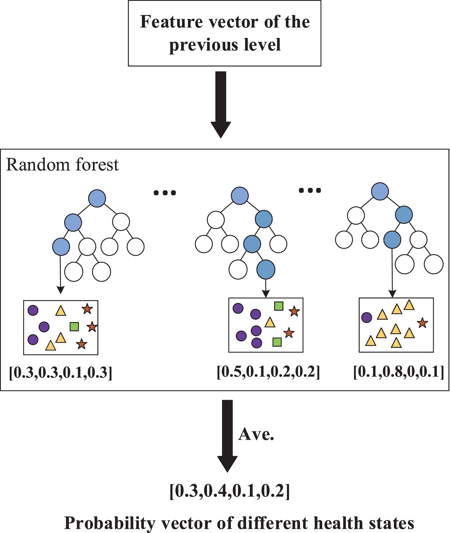
The generation process of different health states probability vector.

Fig. 5

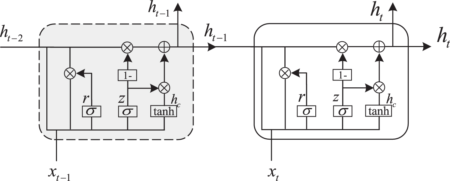
The GRU network structure.

Fig. 6

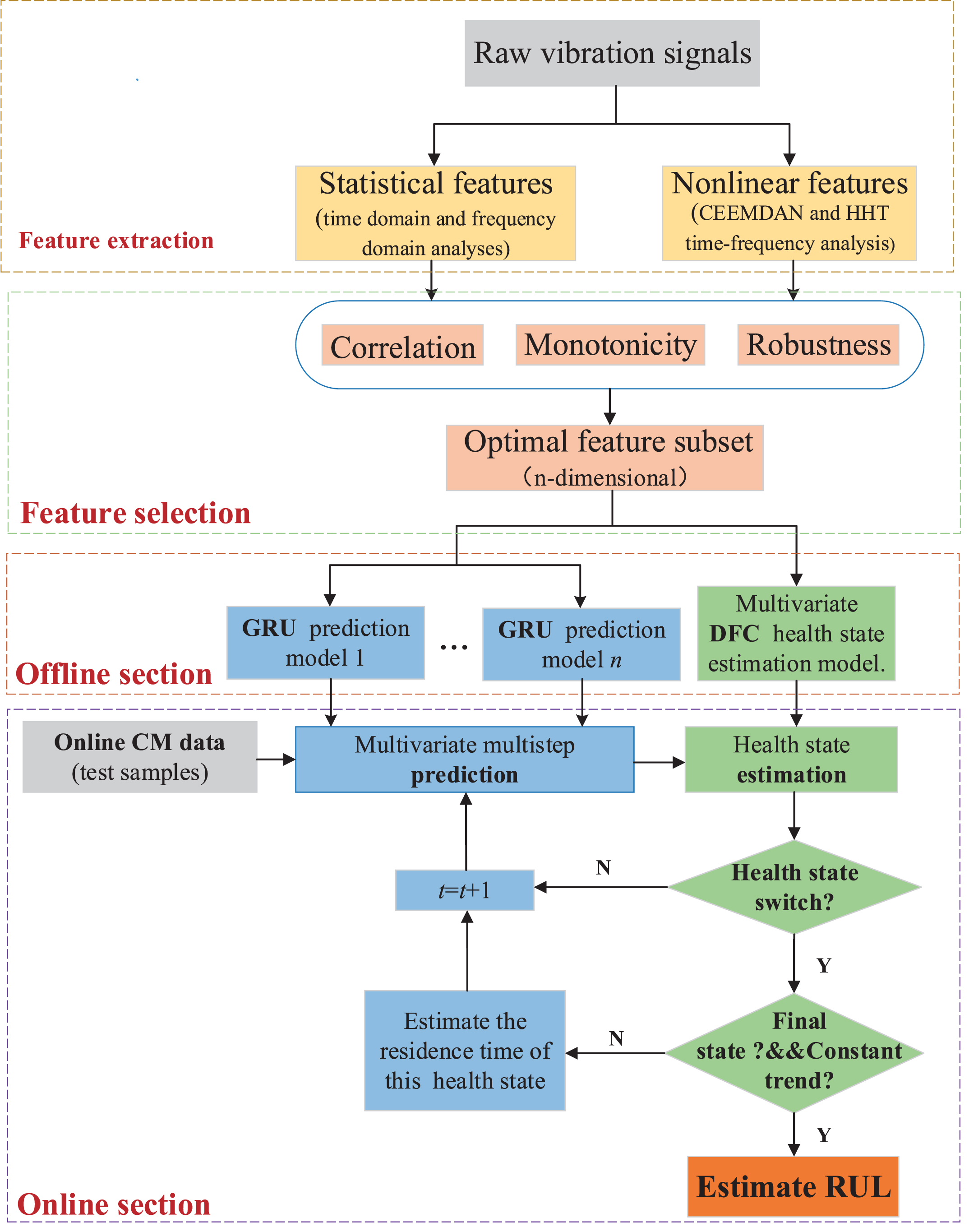
Detailed process of the online RUL prognostics.

In this paper, the error of online RUL prognostics is calculated as $E r_{m} (%) = \frac{RU L_{m} - {\hat{RUL}}_{m}}{RU L_{m}} * 100$ (29) where RUL_m and ${\hat{RUL}}_{m}$ are the real RUL and the predicted one of the m th testing sample respectively. Er_m > 0 represents the lead prediction, Er_m = 0 represents the on-time prediction, Er_m < 0 represents the lagged prediction. In practical applications, lead prediction is better than lagged prediction, because the former can avoid the equipment failures to a greater extent [35].

4 Experiments, results and discussion

4.1 Description of run-to-failure data

The aim of this section is to illustrate the effectiveness of the proposed approach with the run-to-failure datasets (XJTU-SY) [36] of REBs. The datasets were obtained from a laboratory experimental platform of Xi‘an Jiaotong University and the REBs testbed is shown in Fig. 6.

Table 2 lists the 15 REBs which are tested under 3 different operating conditions. Each condition contains 5 complete run-to-failure subsets, where, the first three subsets are used as the training dataset, and the remaining subsets are used as the testing dataset. The sampling frequency is 25.6 kHz, and 32768 samples (i.e., 1.28 s) can be recorded in 1 min. The experiment will be terminated once the vibration signal amplitude is higher than 20 g (g ≈ 9.8m/s²). The basic parameters of the tested REBs are tabulated in Table 3.

Table 2
Information of the experiment

Operating condition Radial force(kN) Rotating speed(rpm) Training datasets Testing datasets

Condition 1 12 2100 REB1_1 REB1_2 REB1_3 REB1_4 REB1_5

Condition 2 11 2250 REB2_1 REB2_2 REB2_3 REB2_4 REB2_5

Condition 3 10 2400 REB3_1 REB3_2 REB3_3 REB3_4 REB3_5

Operating condition	Radial force(kN)	Rotating speed(rpm)	Training datasets	Testing datasets
Condition 1	12	2100	REB1_1 REB1_2 REB1_3	REB1_4 REB1_5
Condition 2	11	2250	REB2_1 REB2_2 REB2_3	REB2_4 REB2_5
Condition 3	10	2400	REB3_1 REB3_2 REB3_3	REB3_4 REB3_5

Table 3

Basic parameters of the testing rebs

Basic parameter	Value
Inner raceway diameter (D_i)	29.30mm
Outer raceway diameter (D₀)	39.80mm
Pitch diameter (D)	34.55mm
Rolling element diameter (d)	7.92mm
Contact angle (φ)	0º
Number of rolling elements (N_r)	8
Basic dynamic load rating (l_d)	12820N
Basic static load rating (l_s)	6650N

4.2 The result of degradation feature extraction

Moving average method and data standardization technique are performed on the raw vibration signals, and the moving window size is set 20 in this paper. Since the load is added in the horizontal direction, the accelerometer can capture more useful horizontal information. Therefore, the horizontal vibration signals are adopted for degradation prediction of REBs in this paper.

Take the training dataset REB1_1 of condition 1 as an example. First of all, 11 statistical features (F_STA = [F₁, F₂, …, F₁₁]) are extracted by analyzing the time domain and frequency domain signals of REB1_1. Then, CEEMDAN method is utilized to extract the IEFs as Eq. (9), that is, the preprocessed vibration signals of REB1_1 are decomposed into 12 IMFs (F_IEF = [F₁, F₂, …, F₁₁]) and a residue with ensemble number I = 100. After that, 4 FFFs (F_FFF = [F₁, F₂, …, F₁₁]) can be extracted by using HHT method. The frequencies of inner ring, outer ring, rolling element and cage are calculated to be f_i = 172 HZ, f_o = 172 HZ, f_b = 172 HZ and f_c = 172 HZ according to Eq. (17). Fig. 8 shows the Hilbert marginal spectrum of REB1_1. It can be seen that the amplitude of the FFFs change with time. At this point, there are 27 original features (F = F_STA + F_IEF + F_FFF = [F₁, F₂, …, F₂₇]) in total, the training dataset X (3 ×27 × T) and the testing dataset X′ (2 ×27 × T′) can be obtained under each condition.

Fig. 7

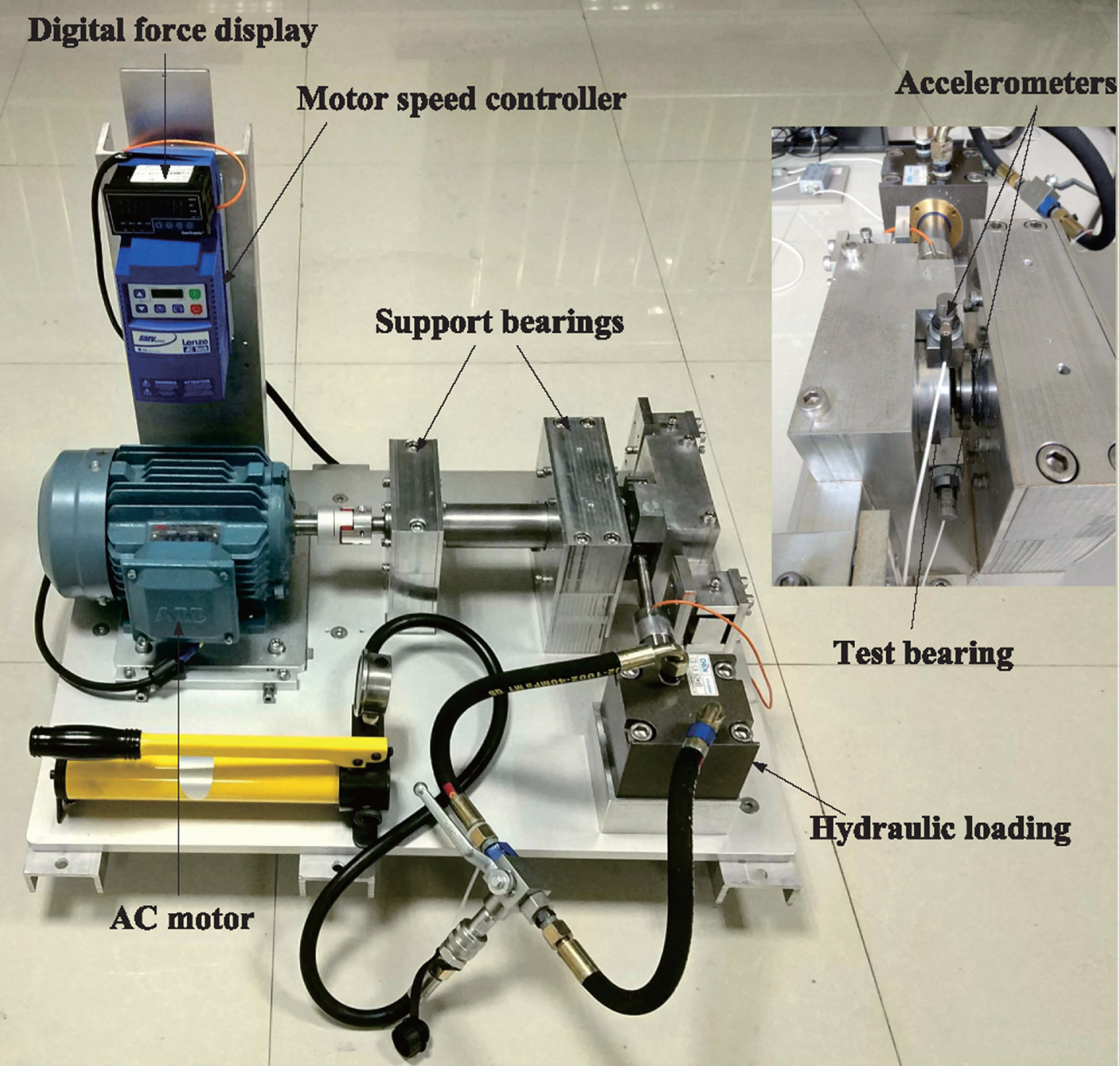
REBs testbed.

Fig. 8

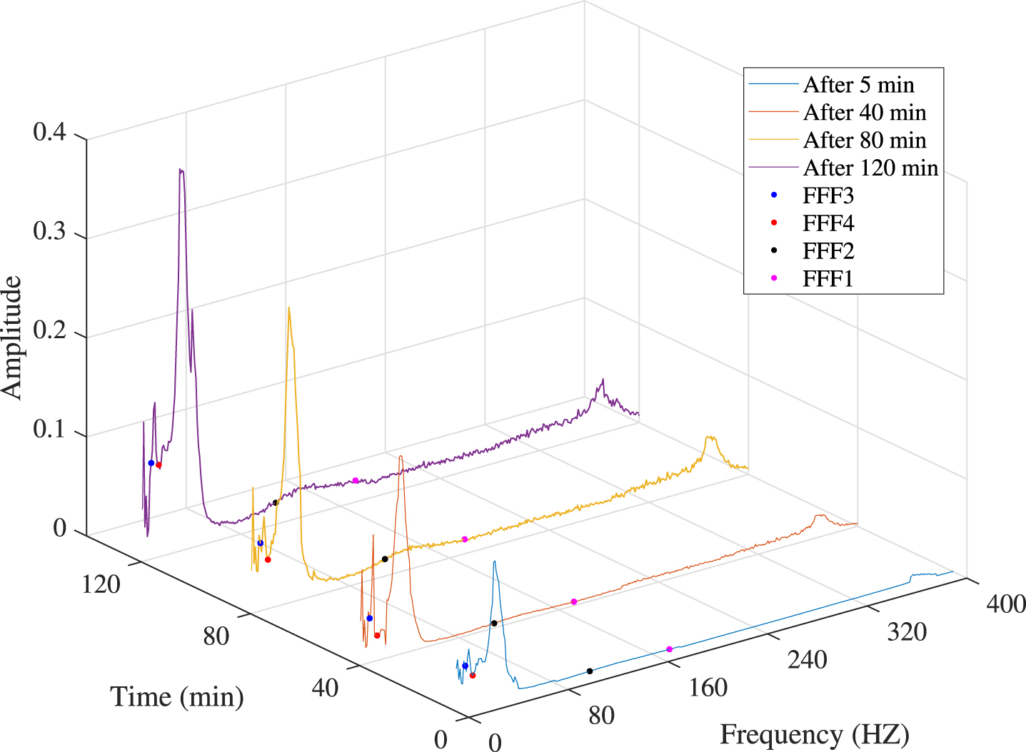
Hilbert marginal spectrum of REB1_1.

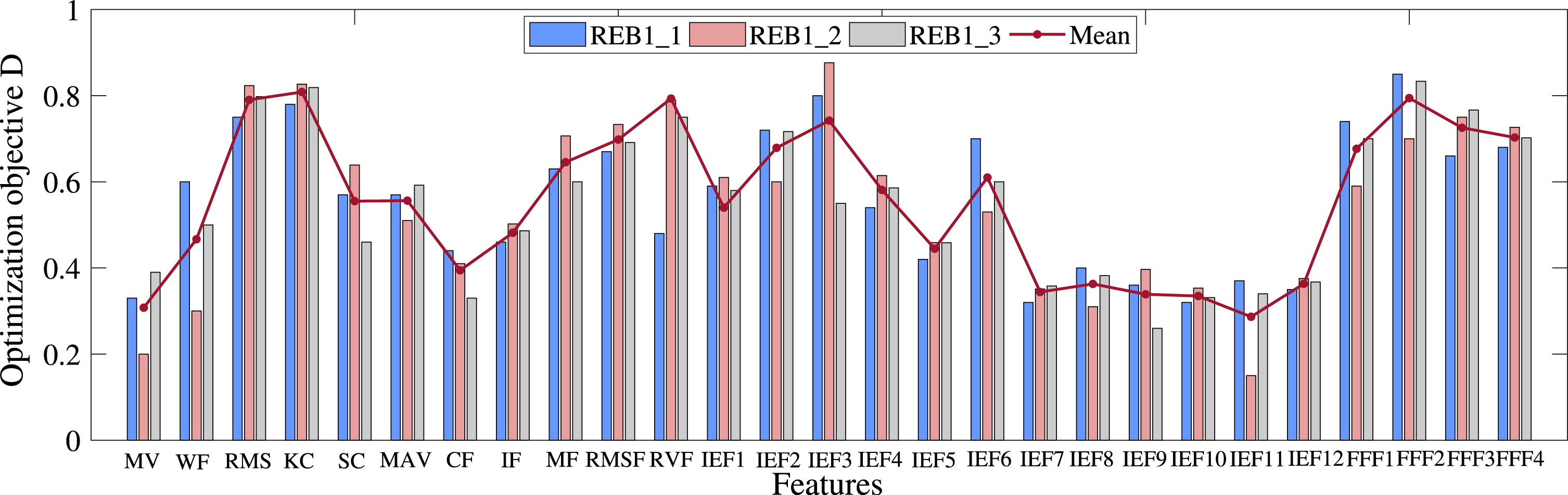
4.3 The result of degradation feature selection

The irrelevant and redundant features can not reflect the degradation information. To increase the accuracy of prediction results, degradation feature selection is implemented in this paper as described in Section II-B. Fig. 9 shows the score of the three training bearings (REB1_1, REB1_2, REB1_3) in condition 1, which can be calculated according to Eq. (22). In this article, the features with D ≥ 0.6 are selected (Fig. 10). Thus, statistical features (i.e., KC, RMS, MF, RVF, RMSF), IEFs (i.e., IEF2, IEF3, IEF6) and FFFs (i.e., FFF1, FFF2, FFF3, FFF4) are picked out, and they are arranged in a 3-D training dataset X (3 ×27 × T).

4.4 The result of offline health state assessment

As discussed in Section II-C, the 3-D dataset $\tilde{X} (3 \times 12 \times T) (T \in [123, 161])$ in condition 1 can be unfolded into a 2-D dataset $\bar{X} (442 \times 12)$ . Set the number of health states C = 4. Algorithm 1 is implemented to assign health status labels “1”, “2”, “3” and “4” to the health state, mild degradation state, moderate degradation state and near-failure state, respectively. The cut-off distance d_c is set 0.2 according to [32].

The parameters of Algorithm 3, 12 Offline Health State Assessment Modeling Based on DF Classifier are set as [33]: n _ forests = 2, n _ estimators = 101, t _ accuracy = 90. Then, an offline health state assessment model can be established. Fig. 11 and Fig. 12 illustrate assessment results of REB1_1 and REB1_2 respectively. Fig. 11(a) and Fig.12(a) are the health state labels of the REBs, and Fig. 11(b) and Fig. 12(b) are the corresponding confidence levels. It can be seen that REB1_1 and REB1_2 are in two different initial states. Instead of assuming that all REBs are in the same initial condition, the proposed method can classify the initial state accurately. Therefore, Hypothesis 1 is well fulfilled.

Fig. 9

Optimization objective D of the three training REBs.

Fig. 10

Optimization objective of original features.

Fig. 11

Health state assessment result of REB1_1. (a) Assessment result.(b) Confidence level.

Fig. 12

Health state assessment result of REB1_2. (a) Assessment result.(b) Confidence level.

4.5 The result of offline degradation trend prediction model and online RUL prognostics

According to Algorithm 3, 12 Offline Degradation Trend Prediction Modeling Based on GRU, 12 offline degradation trend predictors are established respectively. Then, the online RUL prognostics can be finished by combining the offline health state assessment model and offline degradation trend prediction model. Take the testing dataset of REB1_4 as an example. Fig. 13 (a)-(l) show the results of the degradation trend prediction and Fig. 14 illustrates the results of the health state assessment. The prediction starts at the 41st minute, and the actual data in Fig. 14 are not smoothed, so as to distinguish them from the prediction results. When the health state of REB1_4 changes to the last state and the degradation trend of FFF2 is constant, the prognostics is terminated. It can be calculated that the residence time of the health state, mild degradation state, moderate degradation state and near-failure are 28 min, 36 min, 13 min and 7 min respectively. The predicted RUL of REB1_4 is 78 min, while the actual RUL is 82 min. Therefore, Hypothesis 2 is well fulfilled.

Fig. 13

Results of the degradation trend prediction of REB1_4.

Fig. 14

Health state assessment result of REB1_2. (a) Assessment result. (b) Confidence level.

Five existing methods are employed to compared with the proposed approach. The prediction errors of these methods can be calculated according to Eq. (29), which are shown in Table 4. The experimental results indicate that there is no lagged prediction in the proposed method. Moreover, the prognostics accuracy of the proposed approach is higher than other listed methods.

Table 4

Prediction errors of six testing rebs

Method	REB1_4 (%)	REB1_5 (%)	REB2_4 (%)	REB2_5 (%)	REB3_4 (%)	REB3_5 (%)
Proposed method	4.8	0.55	1.13	5.2	7.5	1.63
Direct method [14]	-13.9	26.7	/	/	/	/
Univariate method [16]	/	/	-1.4	/	/	39.3
Multivariate method [18]	2.6	-34.2	/	/	/	/
Multivariate method [24]	-19.3	/	0.7	-25.5	/	17.7
Multivariate method [25]	/	1.6	-30.5	9.4	/	-29.5

5 Conclusion

This paper proposes a novel four-step data-driven degradation prognostics strategy based on the multivariate deep forest (DF) classifier and GRU network for REBs. In the first step, multiple degradation features are extracted from the raw vibration signals, consisting of statistical features, intrinsic energy features (IEFs) and fault frequency features (FFFs). In the second step, the sensitive fault features are selected according to the monotonicity, correlation and robustness metrics. In the third step, a multivariate DF based health state assessment model and GRU based multistep degradation trend prediction model are established. In the final step, the above two models are combined to estimate the RUL of REBs. The verification results show that the proposed approach achieves good performance and has great superiority over the existing major approaches. The proposed approach takes into account initial condition uncertainty and does not need to preset a FT. Meanwhile, the residence time in different health states of the REBs can be calculated. Therefore, the proposed method is beneficial for formulating the flexible maintenance strategy of REBs. In this way, the waste of resources can be reduced in a large extent.

The research in this article assumes that the REBs have a constant working environment. However, in practical applications, the working environment of REBs may change. In the future, the REBs will be considered as a multiparameter hybrid system combining with the physics-based prognostics methods to study the RUL prediction under changing conditions.

References

Cheng

Z.W.

, and C.B, Predicting the remaining useful life of rollingelement bearings using locally linear fusion regression, Journal of Intelligent & Fuzzy Systems 34(6) (2018), 1875–8967.

Lin

Q.B.

, Xu

Z.F.

and Lin

, State of health estimation and remaining useful life prediction for lithium-ion batteries using fbelnn and rcmnn, Journal of Intelligent & Fuzzy Systems 40(6) (2021), 10919–10933.

Qin

, Chen

, Xiang

and Zhu

, Gated dual attention unitneural networks for remaining useful life prediction of rollingbearings, IEEE Transactions on Industrial Informatics 17(9) (2021), 6438–6447.

Bertolino

A.C.

, Sorli

, Jacazio

and Mauro

, Lumped parameters modelling of the emas’ ball screw drive with special consideration to ball/grooves interactions to support model-based health monitoring, Mechanism and Machine Theory 137 (2019), 188–210.

Liu

and Shao

Y.M.

, Overview of dynamic modelling and analysis ofrolling element bearings with localized and distributed faults, Nonlinear Dynamics 93(4) (2018), 1765–1798.

Lei

Y.G.

, Li

N.P.

, Gontarz

, Lin

, Radkowski

and Dybala

, A model-based method for remaining useful life prediction ofmachinery, IEEE Transactions on Reliability 65(3) (2016), 1314–1326.

Wang

Z.Q.

, Hu

C.H.

and Fan

H.D.

, Real-time remaining useful life prediction for a nonlinear degrading system in service: Applicationto bearing data, IEEE/ASME Transactions on Mechatronics 23(1) (2017), 211–222.

Guo

, Li

N.P.

, Jia

, Lei

Y.G.

and Lin

, A recurrent neural network based health indicator for remaining useful life predictionof bearings, Neurocomputing 240 (2017), 98–109.

, Ding

and Sun

J.Q.

, Remaining useful life estimation in prognostics using deep convolution neural networks, ReliabilityEngineering & System Safety 172 (2018), 1–11.

10.

Nuhic

, Terzimehic

, Soczka-Guth

, Buchholz

and Dietmayer

, Health diagnosis and remaining useful life prognostics oflithium-ion batteries using data-driven methods, Journal ofPower Sources 239 (2013), 680–688.

11.

Ben Ali

, Chebel-Morello

, Saidi

, Malinowski

and Fnaiech

, Accurate bearing remaining useful life prediction based onweibull distribution and artificial neural network, MechanicalSystems and Signal Processing 56-57 (2015), 150–172.

12.

Zhao

, Wang

D.Z.

, Yan

R.Q.

, Mao

K.Z.

, Shen

and Wang

J.J.

, Machine health monitoring using local feature-based gated recurrentunit networks, IEEE Transactions on Industrial Electronics 65(2) (2018), 1539–1548.

13.

Javed

, Gouriveau

and Zerhouni

, State of the art and taxonomy of prognostics approaches, trends of prognosticsapplications and open issues towards maturity at differenttechnology readiness levels, Mechanical Systems Signal Processing 94(15) (2017), 214–236.

14.

Joshi

and Patil

, Prediction of surface roughness by machine vision using principal components based regression analysis, Procedia Computer Science 167 (2020), 382–391.

15.

Schwendemann

, Amjad

and Sikora

, A survey of machine-learning techniques for condition monitoring and predictive maintenance of bearings in grinding machines, Computers inIndustry 125 (2021).

16.

Akpudo

U.E.

and Hur

J.-W.

, A feature fusion-based prognosticsapproach for rolling element bearings, Journal of MechanicalScience and Technology 34(10) (2020), 4025–4035.

17.

Chen

W.D.

, Liang

, Yang

Z.H.

and Li

, A Review of Lithium-Ion Battery for Electric Vehicle Applications and Beyond 158 (2019), 4363–4368.

18.

Javed

, Gouriveau

and Zerhouni

, A new multivariate approachfor prognostics based on extreme learning machine and fuzzyclustering, IEEE Transactions on Cybernetics 45(12) (2015), 2626–2639.

19.

Dragomir

O.E.

, Gourtveau

, Zerhouni

and Dragomir

, Framework for a distributed and hybrid prognostic system, IFACProceedings Volumes 40(18) (2007), 431–436.

20.

Emmanuel,

Ramasso

, Michèle,

Rombaut

, Noureddine and Zerhouni , Joint prediction of continuous and discrete states in time-seriesbased on belief functions, IEEE Transactions on Cybernetics 43(1) (2013), 37–50.

21.

Wang

, Peng

Y.Z.

, Zi

Y.Y.

, Jin

X.H.

and Tsui

K.L.

, A two-stagedata-driven-based prognostic approach for bearing degradationproblem, IEEE Transactions on Industrial Informatics 12(3) (2016), 924–932.

22.

Ramasso

and Gouriveau

, Remaining useful life estimation byclassification of predictions based on a neuro-fuzzy system andtheory of belief functions, IEEE Transactions on Reliability 63(2) (2014), 555–566.

23.

Xia

, Li

, Shu

T.X.

, Wan

J.F.

, de Silva

C.W.

and Wang

Z.R.

, A two-stage approach for the remaining useful life prediction ofbearings using deep neural networks, IEEE Transactions onIndustrial Informatics 15(6) (2019), 3703–3711.

24.

Soualhi

, Medjaher

and Zerhouni

, Bearing health monitoringbased on hilbert-huang transform, support vector machine, andregression, IEEE Transactions on Instrumentation andMeasurement 64(1) (2015), 52–62.

25.

Xiahou

T.F.

, Zeng

Z.G.

and Liu

, Remaining useful life prediction by fusing expert knowledge and condition monitoring information, IEEE Transactions on Industrial Informatics 17(4) (2021), 2653–2663.

26.

Zhao

, Yan

R.Q.

, Chen

Z.H.

, Mao

K.Z.

, Wang

and Gao

R.X.

, Deep learning and its applications to machine health monitoring, Mechanical Systems and Signal Processing 115(15) (2019), 213–237.

27.

G.J.

, Hou

D.M.

, Qi

H.Y.

and Bo

, High-speed train wheel setbearing fault diagnosis and prognostics: A new prognostic modelbased on extendable useful life, Mechanical Systems and SignalProcessing 146 (2021).

28.

Elbouchikhi

, Choqueuse

, Amirat

and Benbouzid

M.E.H.

, and S.Turri, An efficient hilbert–huang transform-based bearingfaults detection in induction machines, IEEE Transactions onEnergy Conversion 32(2) (2017), 401–413.

29.

, Wu

, Cao

, Or

S.W.

, Deng

and Shao

, Degradation data-driven time-to-failure prognostics approach for rolling elementbearings in electrical machines, IEEE Transactions onIndustrial Electronics 66(1) (2019), 529–539.

30.

Q.H.

, Ding

K.Q.

and Huang

B.Q.

, Approach for fault prognosisusing recurrent neural network, Journal of Intelligent Manufacturing 31(7) (2020), 1621–1633.

31.

, Wu

, Lv

, Deng

and Shao

, Design a degradationcondition monitoring system scheme for rolling bearing using emd andpca, Industrial Management Data Systems 117(4) (2017), 713–728.

32.

Rodriguez

and Laio

, Clustering by fast search and find of density peaks, Science 344(6191) (2014), 1492–1496.

33.

Zhou

Z.H.

and Feng

, Deep forest, Nat Sci Rev 6(1) (2019), 74–86.

34.

Choi

, Schuetz

, Stewart

W.F.

and Sun

J.M.

, Using recurrent neural network models for early detection of heart failure onset, Journal of the American Medical Informatics Association 24(2) (2017), 361–370.

35.

Yan

and Wei

X.K.

, RUL Prediction for Bearings Based on Fault Diagnosis 482 (2018), 1013–1020.

36.

Wang

, Lei

, Li

and Li

, A hybrid prognostics approach for estimating remaining useful life of rolling element bearings, IEEE Transactions on Reliability 69(1) (2018), 401–412.

A data-driven degradation prognostics approach for rolling element bearings

Abstract

Keywords

1 Introduction

3.1 Step 1: Degradation feature extraction

3.1.1 Statistical features extracted by time domain and frequency domain analyses

4.1 Description of run-to-failure data

Table 2 Information of the experiment Operating condition Radial force(kN) Rotating speed(rpm) Training datasets Testing datasets Condition 1 12 2100 REB1_1 REB1_2 REB1_3 REB1_4 REB1_5 Condition 2 11 2250 REB2_1 REB2_2 REB2_3 REB2_4 REB2_5 Condition 3 10 2400 REB3_1 REB3_2 REB3_3 REB3_4 REB3_5

4.4 The result of offline health state assessment

References

Table 2
Information of the experiment

Operating condition Radial force(kN) Rotating speed(rpm) Training datasets Testing datasets

Condition 1 12 2100 REB1_1 REB1_2 REB1_3 REB1_4 REB1_5

Condition 2 11 2250 REB2_1 REB2_2 REB2_3 REB2_4 REB2_5

Condition 3 10 2400 REB3_1 REB3_2 REB3_3 REB3_4 REB3_5