Prior latent distribution comparison for the RNN Variational Autoencoder in low-resource language modeling

Abstract

Probabilistic Bayesian methods are widely used in the machine learning domain. Variational Autoencoder (VAE) is a common architecture for solving the Language Modeling task in a self-supervised way. VAE consists of a concept of latent variables inside the model. Latent variables are described as a random variable that is fit by the data. Up to now, in the majority of cases, latent variables are considered normally distributed. The normal distribution is a well-known distribution that can be easily included in any pipeline. Moreover, the normal distribution is a good choice when the Central Limit Theorem (CLT) holds. It makes it effective when one is working with i.i.d. (independent and identically distributed) random variables. However, the conditions of CLT in Natural Language Processing are not easy to check. So, the choice of distribution family is unclear in the domain. This paper studies the priors selection impact of continuous distributions in the Low-Resource Language Modeling task with VAE. The experiment shows that there is a statistical difference between the different priors in the encoder-decoder architecture. We showed that family distribution hyperparameter is important in the Low-Resource Language Modeling task and should be considered for the model training.

Keywords

Bayesian model low-resource language modeling NLP priors RNN VAE Variational Autoencoder

1 Introduction

Bayesian methods in machine learning have recently gained more popularity. The estimations in Bayesian models are considered as distributions rather than points. It is known as Bayesian inference. Less formally, it is a concept, which considers parameters of statistical models as random variables from the given distribution family.

The intuition behind such approaches often lies in splitting complex structures into chunks that are easier to explain and adding new informative features. These chunks are usually referred to as latent variables. A latent variable is a piece of information hidden from the initial datapoints but can boost the model’s accuracy if retrieved. However, in a majority of cases, they are unavailable but can be estimated.

The distribution parameters are fitted on available data. But it is still very unclear for researchers the prior distribution choice for the parameters. Usually, the prior distribution is selected by computational or intuitive logic rather than by strong and formal arguments. Nevertheless, there are a wide variety of different distributions. As a result, the issue remains unsolved.

Language modeling (LM) is a task in the Natural Language Processing field that consists of different methods and algorithms to generate a sequence of tokens. The main problem here for classical algorithms lies in time structure and the complexity of token relations.

The estimation and modeling of tokens’ relationships can be a difficult task. A dataset should cover as many as possible cases of tokens’ usage. With limited resources, it is practically never the case. NLP datasets show lack of representativity for most of the tokens. This problem is a major challenge for classic methods based on the Maximum Likelihood Estimation (MLE) methodology. It is known that useful properties of MLE estimations (e.g., consistency, asymptotic normality) remain when a number of samples are much more than a number of model parameters. In other words, to use the MLE estimations effectively, one needs plenty of data. For Natural Language Processing tasks gathering a representative dataset is a nontrivial problem. On the other hand, Bayesian inference estimations work with a smaller amount of data better.

Language modeling tasks became a much more popular problem for the industry to solve after the introduction of Recurrent Neural Networks (RNN). These tasks appear in modern industries all over the domains: chat-bots, question-answering, machine translation, etc. However, the LM model can hardly be trained on tasks, with only a small dataset available compared to the number of model parameters. For example, Low-Resource Language Modeling (LRLM). LRLM is applicable in cases where texts are presented in small amounts or missing. Moreover, in unusual or new tasks, datasets cannot be built in a reasonable time and will probably take many resources. For instance, there are a lot of languages that lack quality datasets. Another example is a translation task. It is not easy to find a big dataset where the same text is presented in both languages and covers the majority of cases in terms of representativity. This issue is particularly important in LRLM.

In this work, we compared a list of prior distributions in the Variational Autoencoder (VAE) architecture based on the encoder-decoder approach. We fixed all the layers’ dimensions but latent generator to test how the selection of prior distribution for a latent variable can affect the final model score in the case of the LRLM task. We focused on continuous distributions because it is possible to find a homotopy between samples with this constraint.

The paper is structured as follows. The problem is stated in Section 1. In Section 2, the overview of previous works is presented. Then in Section 3, we provide background information regarding families of distributions. In Section 4, the training objective, model architecture, and hyperparameters are discussed. Details regarding dataset gathering and preprocessing are provided in Section 5. Further in Section 6, the final results are discussed. Finally, conclusions are drawn in Section 7.

2 Related work

Variational Bayes Auto-Encoding [1] is a methodology that can provide additional benefits for the learning process:

A way of regularization.

The possibility of sampling points from the latent space, which is obtained by the generative model.

The possibility of storing high-level structure of the space over homotopy.

A prior distribution plays an important role in Bayesian statistics. The choice of a prior distribution can give different results, especially when the number of samples is relatively small. In addition, empirical results show that the appropriate prior selection improves the quality of hidden representations [2 –4].

The embedding pre-training is an optimal procedure for obtaining the best results. However, high scores cannot be obtained even with it in some tasks. For example, it is quite challenging for BERT [5] to solve the task optimally without fine-tuning. Moreover, BERT even can show worse results than the classical word2vec model [6]. This issue was discussed in Ref. [7].

On the other hand, fine-tuning on a small dataset can lead to overfitting. There are different approaches to solving such problems. They can be split into two main categories:

Adding additional pre-training tasks (like was proposed in ERNIE [8] or in Ref. [9] and Ref. [10]), which are connected to a downstream task more directly than the masking language modeling task.

Fine-tuning on a small set of parameters only (like was proposed in Albert [11]).

Pre-training proved to be an efficient approach to a majority NLP tasks. It requires one big and representative model that is tuned for a new objective. On the other hand, it is much harder to fight to overfit when it comes to small data. Adding additional pre-training tasks can reduce this problem. But it also creates new challenges: pre-trained tasks should be selected beforehand, and it is not clear which ones will increase quality. Furthermore, different fitting objectives will take a lot of time and resources, while going over different distribution families requires less apriori knowledge.

Similar issues arise with fine-tuning on a small set of parameters. The set selection usually is performed experimentally and by checking all possible combinations. It consumes a lot of time and resources. Yet, another relevant approach should be considered via regularization of the embedding space with the VAE. In our case, regularization of the model parameters are performed via a selection of an appropriate prior.

Ref. [12] proposed a new framework for the generation of sentences from the latent space. This framework was developed as an auto-regressive model with the seq2seq architecture based on Ref. [13], and it gives some theoretical insights about architecture selection. However, they did not analyze which prior family could perform better, maintaining the discriminant information of the vocabulary distribution. Additional work in this field was done in Ref. [13], but text generation with other architectures showed that the generated sentences were not coherent or grammatically correct. Moreover, such representation could not store high-level text structures: sentiment, authenticity, etc.

A similar analysis is performed in Ref. [14] for the Bayesian skip-gram model on a word level. The results showed improvement in text recovery and downstream tasks. So, the question about distribution of the whole sequence embedding can be raised.

3 Latent distributions

We considered the normal, the log-normal, and the Cauchy distributions as the latent ones in this work.

3.1.1 Normal distribution

Normally distributed random variable $X \sim N (μ, σ^{2})$ can be reparametrized by the following Equation (1): $X \sim μ + σ N (0, 1) .$ (1) From Ref. [15], the Kullback-Leibler divergence (KLD) can be calculated as in Equation (2):

$\begin{matrix} D_{KL} (N (μ, σ^{2}) ∥ N (0, 1)) \\ = - \frac{1}{2} (1 + log (σ^{2}) - μ^{2} - σ^{2}) . \end{matrix}$ (2)

3.1.2 Log-normal Distribution

Reparametrization trick for the log-normal variable $X \sim Log N (μ, σ^{2})$ is calculated in the same way, as for the normal one, but with additional exponent (Equation (3)): $X \sim e^{μ + σ N (0, 1)} .$ (3)

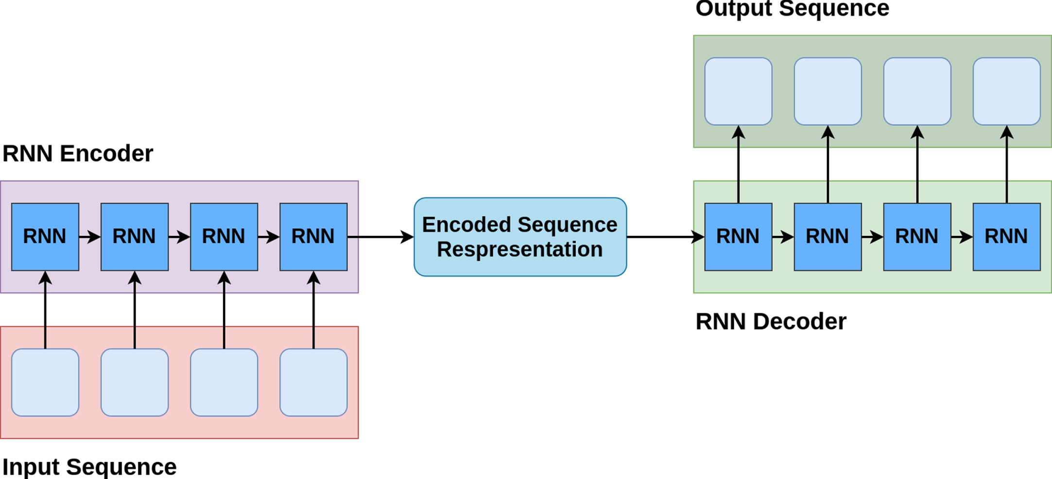
From Ref. [15], KLD is the same as for the $N$ . The major difference between the log-normal and the normal distribution is its shape, caused by the exponential transformation. The normal distribution is symmetrical, but the log-normal distribution is not. Values in the log-normal distribution are positive.

Fig. 1

Encoder-Decoder architecture. The input sequence is encoded in the representation (fixed-dimensional vector). Then the decoder generates from this representation step-by-step output sequence.

3.1.3 Cauchy Distribution

The Cauchy distribution looks very similar to the normal distribution, but it has heavy tails. It is also symmetrical, but the mean and the variance cannot be calculated directly –the corresponding integrals do not converge. The Cauchy distributed variable (μ, σ) can be reparametrized with a Uniform distributed variable U (0, 1) with the Equation (4): $Cauchy (μ, σ) \sim μ + σ tan (π (U (0, 1) - \frac{1}{2})) .$ (4)

From Ref. [16], KLD can be calculated by the following Equation (5): $\begin{matrix} D_{KL} (Cauchy (μ, σ) ∥ Cauchy (0, 1)) = \\ = log \frac{(σ + 1)^{2} + μ^{2}}{4 σ} . \end{matrix}$ (5)

Heavy tails of the Cauchy distribution can be viewed as additional regularization. Also, it seems that they may model a more flexible latent space for the model.

4 Model training

4.1 Encoder-decoder architecture

The encoder-decoder approach impacted NLP, creating state-of-the-art results in a large number of tasks. For example, in translation task was a major breakthrough. The encoder-decoder model can be built in different ways. The one we are using consists of two RNN blocks that are applied one by one: encoder and decoder. It is the most classical way to use architecture. Nevertheless, it is proven to be effective. The encoder takes as an input a sequence of tokens and encodes it into a fixed-sized vector. This vector contains all the necessary information regarding an input sequence. The decoder then samples one by one the tokens, given the vector representation from the encoder (see Fig. 1).

The advantage of this model is in its ability to work with a non-fixed number of tokens due to the RNN nature. This property makes it convenient to use in the translation and generation domains. On the other hand, RNN has a vanishing gradient problem, which results in a quality loss on long sequences.

4.2 VAE

Consider dataset X = {X_i, i = 1, . . . , N}, where X_i - i.i.d. (independent and identically distributed) samples. The method assumes that each datapoint X can be sampled from some unknown random process with unobserved variable Z. We will call Z latent variable. So, in order to sample X, we need to sample Z from some p (Z|θ) and then sample X from p (X|Z, θ). Both prior p (Z|θ) and likelihood p (X|Z, θ) are assumed to be from parametric distribution families p (Z) and p (X|Z) respectively. Let q (Z|λ) be an estimation of p (Z).

The parameter vector is then optimized by Maximum Likelihood Estimation (MLE) as in Equation (6): $\begin{matrix} log p (X | θ) & = L (λ, θ, X_{i}) \\ + D_{KL} (q (Z | X_{i}, λ) ∥ p (Z | X_{i}, θ)), \end{matrix}$ (6) where $L (λ, θ, X_{i}) = - D_{KL} (q (Z | X_{i}, λ) ∥ p (Z | θ)) + E_{q (Z | X_{i}, λ)} (log p (X_{i} | Z, θ))$ . Model is trained both to approximate Z distribution and simultaneously learn the p (X|Z). Detailed optimization algorithm is introduced in Ref. [1].

4.3 Token masking and preprocessing

Token masking is a token replacement with the special mask token (<MASK>). The token masking is defined in the following way: the uniform random value is sampled for each token. Then it is compared with the threshold (mask probability), and if the sampled value is less than the mask probability, the token would be masked (see Fig. 2). The value selection of the mask probability is described in the Experiments section. Token unmasking is the main training objective to achieve high-quality token representation via its surrounding context. The effectiveness of the approach was proven in Refs. [5 , 10–12].

Fig. 2

Token masking example. For each token, the uniform random value is sampled. Then it is compared with the threshold (mask probability, which in the example equals 0.5), and if the sampled value is greater than the mask probability, the token would be masked.

In order to make the masking procedure more robust, we considered the mask probability as the percent of the sequence to be masked and masked this exact number of tokens rounded up. On average, this procedure is equivalent to the above-mentioned procedure.

Each token is encoded with the Bag-of-Words approach. In vocabulary, we fix special additional tokens –start-of-sequence, end-of-sequence, mask, and padding.

4.4 Model architecture

To perform analysis, we use encoder-decoder architecture highly inspired by Ref. [12]. As inputs, the model takes sequences of tokens, where tokens are masked with the probability m and original sequences without masking. Then the embedding layer is applied for both masked and unmasked sequences. The unmasked sequence is passed through the encoder RNN to obtain the encoded representation. Encoded representations are used to calculate the parameters of the latent distribution. For the RNN cell, we used Gated Recurrent Unit(GRU). In more detail, latent variable Z is sampled from p (Z|λ, X_E), where X_E is the encoder RNN output, and λ is parameters. As an approximator of λ, we use a feed-forward neural network with fixed hyperparameters and the reparametrization trick.

Sampled Z is viewed as the hidden for the decoder RNN, which takes as inputs embedded masked tokens. Architecture is schematically presented in Fig. 3.

Fig. 3

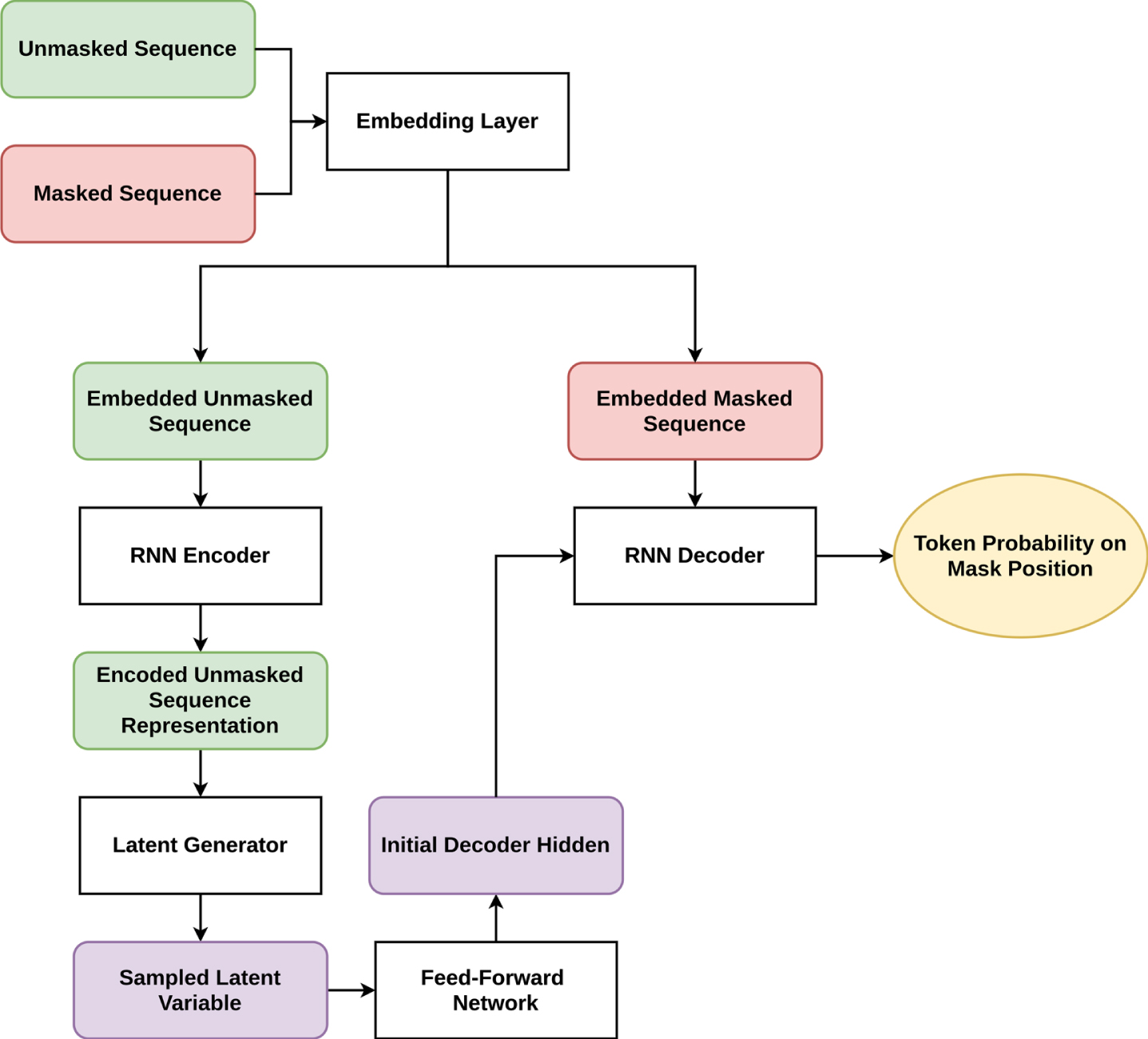
Model architecture. The model takes two sequences: masked and unmasked (original). Then the embedding layer is applied for both masked and unmasked sequences (for each token). The Embedded unmasked sequence is passed through the RNN encoder to obtain the representation of the whole sequence. The parameters of the latent distributions are calculated by the additional model (Latent Generator) from the sequence representation. A sampled latent variable is the initial representation (Initial Decoder Hidden) for the RNN decoder, which takes as inputs embedded masked sequence. The decoder outputs token probability on mask position.

4.5 Additional hyperparameters

Similarly to Ref. [15], we add selection ratio hyperparameter r. The idea is to pass the gradient on randomly selected tokens rather than on the whole reconstructed sequence. The reason for that is that we need to train the decoder to learn the local properties of the sequence. In this way, a better understanding of each token is obtained for mask reconstruction and unmasked tokens.

The mask probability m is also considered as hyperparametr.

4.6 Loss function

The training objective is the reconstruction of sequence with masked tokens (masked language modeling (MLM)). For model optimization, we use Negative Log-Likelihood Loss (NLLLoss) combined with the KLD term.

In Ref. [12], the authors suggest using a weighting mechanism for loss optimization. We also added this weighting mechanism for the KLD part in the loss, which is increasing with time. If the model is trained without weighting, then latent distribution for Z converges too fast. If so, the encoder becomes inefficient. Whatever it returns to decoder, Z is sampled from the same distribution without considering encoder output, returning uninformative vector representation for the decoder. We used the sigmoid approach, provided with Equation (7): $w_{t} = \frac{1}{1 + exp (- k (t - x))} \cdot$ (7)

Here w_t is KLD weight on iteration t. We used k, x hyperparameters same as in Ref. [12].

Final combined loss is calculated with the following Equation (8) (hat stands for estimated values): $\begin{matrix} NLLLoss (({\hat{Y}}_{j}, Y_{j})_{j \in S^{r}})) + \\ w_{t} D_{KL} (\hat{p} (Z | X, λ) ∥ p (Z | θ)) . \end{matrix}$ (8)

Here S^r represents a random selection of r% of merged sequences indexes in batch; ${\hat{X}}_{j}$ is token reconstruction, probability of a token in the position j; Y_j is a token in position j in merged unmasked sequence.

5 Dataset

For the experiments, we used a dataset of COVID-19 related tweets from the Kaggle site 1 and Spanish Poetry dataset from the Kaggle site 2 . The datasets selection was made based on the number of samples criteria and relative density of the vocabulary. For datasets, the following preprocessing was used. Each token was preprocessed with lowercasing. In the case of the Tweet dataset, dropping mentions, emails and hashtags were applied as well. Each token was lemmatized. The vocabulary was built without saving punctuation symbols and stop-words (words that are too common and usually do not have a lexical impact, like articles, prepositions, etc.). We filtered the features, i.e., we considered only those lemmatized tokens that appeared at least 50 times in the corpus. The total vocabulary sizes (with additional symbols):

Tweet dataset: 3,815

Spanish Poetry dataset: 1,527

After that, we considered only sentences that have from 10 to 30 tokens.

Datasets were randomly split into train, validation, and test sets. Datasets are described in Table 1.

Table 1
Datasets statistics

Dataset name Dataset type Number of samples Total number of tokens

Tweet dataset

Train 39,634 463,475

Validation 9,884 115,351

Test 12,268 143,764

Spanish Poetry dataset

Train 13,443 247,309

Validation 3,361 62,270

Test 4,266 78,602

Dataset name	Dataset type	Number of samples	Total number of tokens
Tweet dataset
	Train	39,634	463,475
	Validation	9,884	115,351
	Test	12,268	143,764
Spanish Poetry dataset
	Train	13,443	247,309
	Validation	3,361	62,270
	Test	4,266	78,602

For the validation dataset, we sampled masking for 10% of each sequence. For the test dataset, we applied two mask dropout ratios: 0.1 and 0.5. Measuring model performance on two mask dropout ratios provides additional insights into how well the model can reproduce tokens’ relationships locally and globally. We refer to the model’s ability to reconstruct the distribution of a small number of tokens conditioned on almost all available sequences as tokens’ relationships reproduce locally. By reproducing tokens’ relationships globally, we challenge the model’s ability to reconstruct tokens without sufficient information about a sequence. Less formally, it can be considered as model intuition about the meaning of the sequence.

6 Experiments

As it is impossible to check all of the possible hyperparameters, we selected parameters grid and trained models for 50 epochs for each Z distribution. For the optimization, we used a fixed learning rate and scheduler. We fixed general model architecture for both encoder and decoder RNN and fully connected layers for a latent variable generation. The code and grids can be found on github 3 . At the end of model training, the best state for the (r, m) was selected based on a validation score.

In order to check whether there is a statically significant difference between the results, we used the Wilcoxon signed-rank test of the mean difference. The test was applied for each pair of distributions with corresponding parameters (r, m). The metric used was the accuracy of reconstructed masked tokens. For a p-value adjustment, we used False Discovery Rate (FDR). The results are presented in Table 2, where Priors are pairs of distributions and (0.1) and (0.5) specify test dataset. Consider a space of hyperparameters with fixed family distribution represented by parameters grid. Generally, we do not have any preferences regarding the selection of hyperparameters, so they all be tested. In this case, we can compare if there is a statistical difference between distribution families for different grids. The histograms for all models are presented in Figs. 4 and 5.

Table 2
Wilcoxon signed-rank test results with FDR adjustment

Dataset Priors p-value (0.1) p-value (0.5)

Tweet dataset

Log-Normal - Normal 0.0077 0.0070

Log-Normal - Cauchy 0.0077 0.0285

Normal - Cauchy 0.0033 0.0070

Spanish Poetry dataset

Log-Normal - Normal 0.0117 0.0131

Log-Normal - Cauchy 0.0008 0.0131

Normal - Cauchy 0.0002 0.0012

Dataset	Priors	p-value (0.1)	p-value (0.5)
Tweet dataset
	Log-Normal - Normal	0.0077	0.0070
	Log-Normal - Cauchy	0.0077	0.0285
	Normal - Cauchy	0.0033	0.0070
Spanish Poetry dataset
	Log-Normal - Normal	0.0117	0.0131
	Log-Normal - Cauchy	0.0008	0.0131
	Normal - Cauchy	0.0002	0.0012

Fig. 4

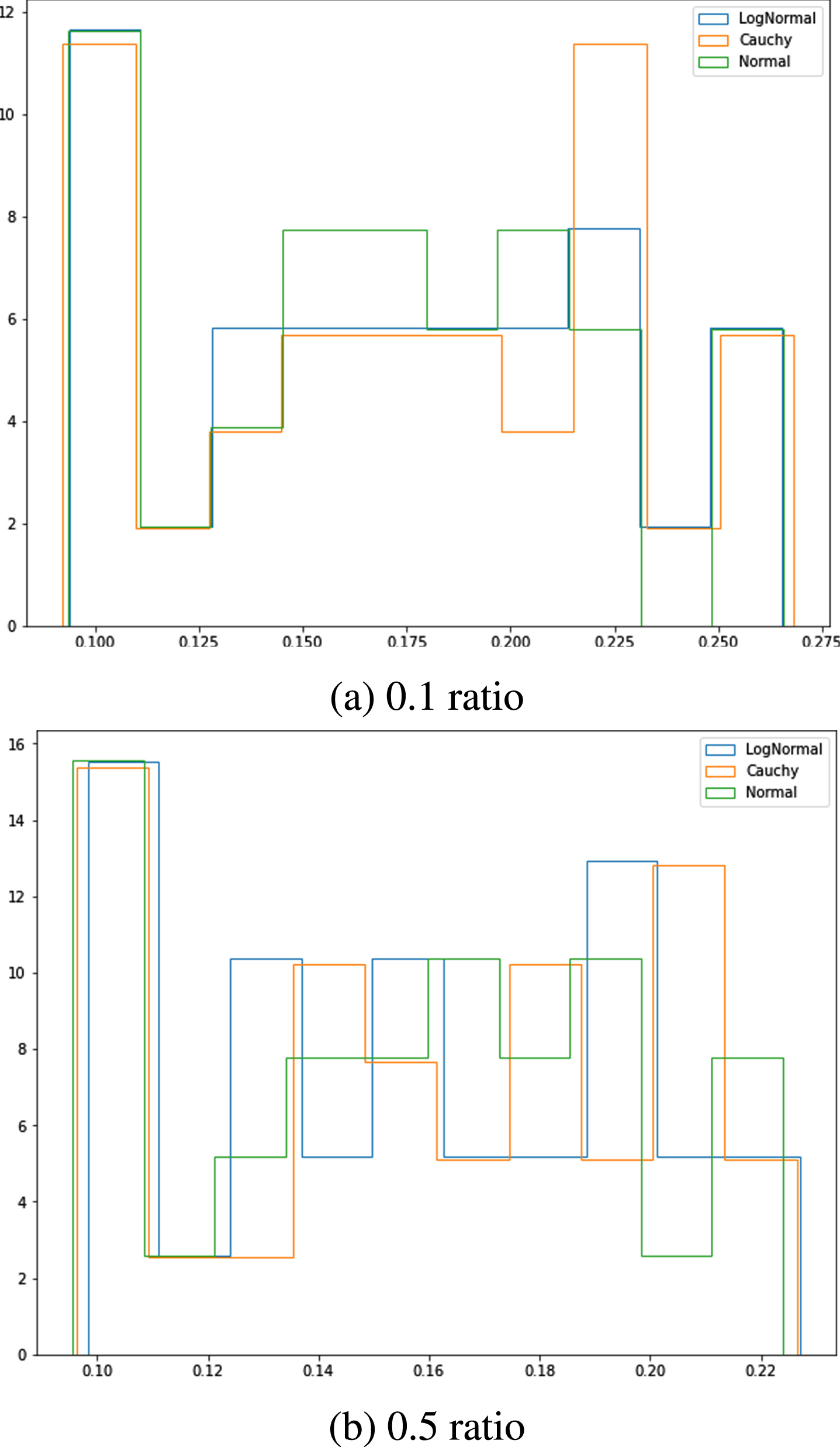
Accuracies of reconstructed masked tokens for Tweet test dataset.

Fig. 5

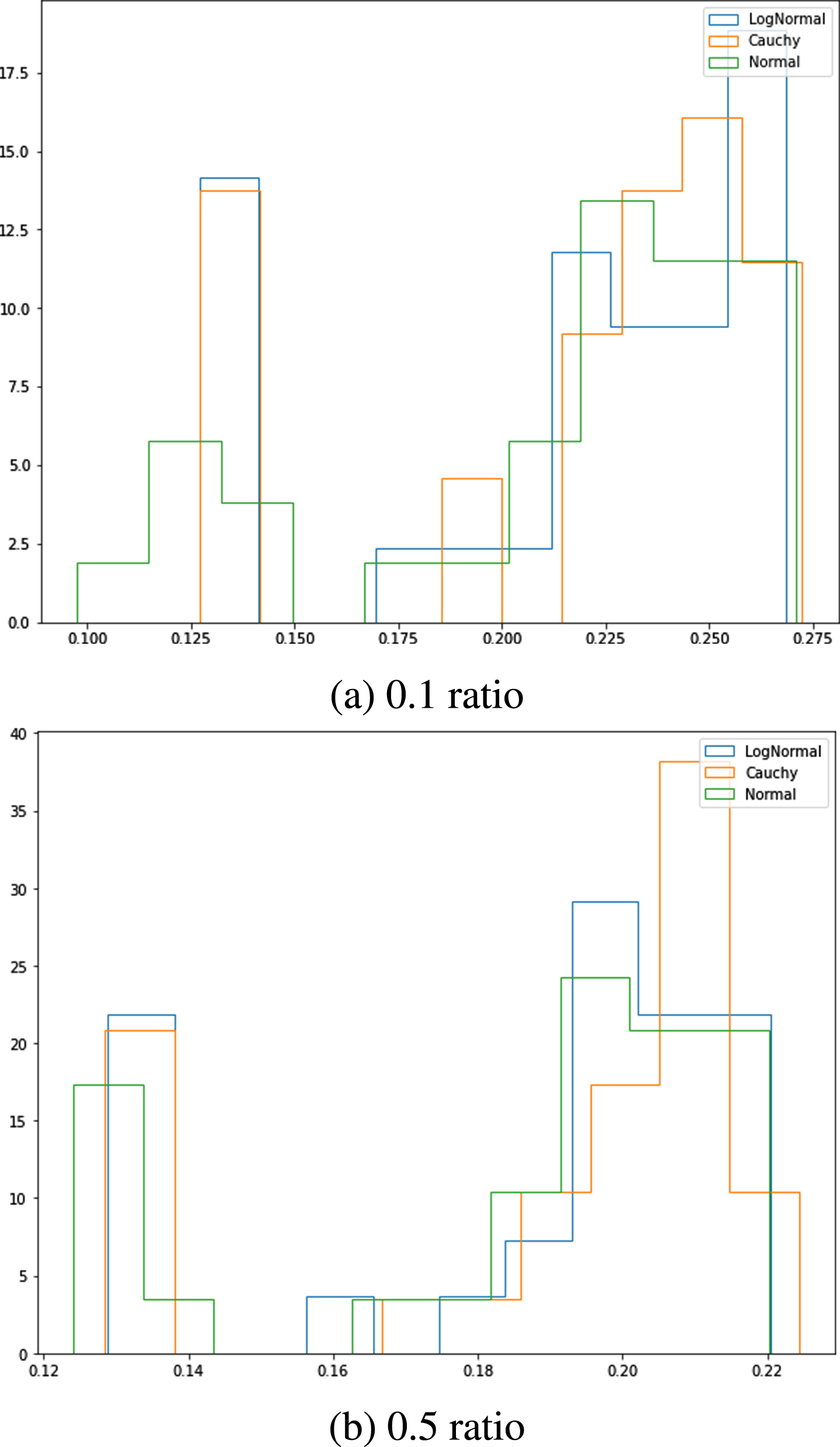
Accuracies of reconstructed masked tokens for Spanish Poetry test dataset

The best mask accuracy scores are presented for each distribution for all test datasets in Table 3. The score was calculated for a model, which has shown the best result on the validation set.

Table 3

Mask accuracy metric per distribution

Dataset	Distr.	SR	MP	MA (0.1)	MA (0.5)
Tweet Dataset
	Cauchy	1.0	0.4	0.2679	0.2217
	Normal	1.0	0.4	0.2656	0.2239
	Log-Normal	1.0	0.4	0.2652	0.2267
Spanish Poetry Dataset
	Cauchy	1.0	0.6	0.2724	0.2243
	Normal	1.0	0.6	0.2711	0.2202
	Log-Normal	1.0	0.4	0.2685	0.2204

The notation is as follows:

SR is selection ratio;

MP is mask probability;

MA is mask accuracy;

(0.1) and (0.5) specifies test dataset.

In our experiments, Wilcoxon test results demonstrate statistical significance. It means that family distribution influences a result without condition on the rest of the parameters grid. Moreover, if there is no opportunity to check a more precise grid, one should focus on the family distribution hyperparameter. The number of possible distributions is discrete and finite. For instance, a selection ratio hyperparameter is continuous, and it is impossible to check all the values.

7 Analysis

The distribution family can also increase the model’s quality with respect to the grid. In our case, we additionally performed the Two Proportion Z-Test on test datasets. For most cases, tests did not show statistical significance due to a small number of samples and a detailed grid. But in the case of the Tweet dataset on 50% of sequence masking, the difference between the best models is significant, specifically on the log-normal and the Cauchy distributions.

This test will show, whether this particular hyperparameter influenced the result unconditioned on the rest of a grid. The results are presented in Table 4. Note that the results are not significant on the test dataset with 10% of sequence masking. In this dataset, the amount of masked tokens per sequence is less than 3, which means we measure a model’s ability to reconstruct a small number of tokens. It means that the changing distribution family does not statistically improve performance locally. With almost all information regarding the sequence, models with different latent distribution families perform similarly.

Table 4
Two Proportion Z-Test results

Dataset Priors p-value (0.1) p-value (0.5)

Tweet dataset

Log-Normal - Normal 0.9442 0.3628

Log-Normal - Cauchy 0.6312 0.0331

Normal - Cauchy 0.6818 0.2224

Spanish Poetry dataset

Log-Normal - Normal 0.7871 0.9840

Log-Normal - Cauchy 0.6818 0.6672

Normal - Cauchy 0.8965 0.64552

Dataset	Priors	p-value (0.1)	p-value (0.5)
Tweet dataset
	Log-Normal - Normal	0.9442	0.3628
	Log-Normal - Cauchy	0.6312	0.0331
	Normal - Cauchy	0.6818	0.2224
Spanish Poetry dataset
	Log-Normal - Normal	0.7871	0.9840
	Log-Normal - Cauchy	0.6818	0.6672
	Normal - Cauchy	0.8965	0.64552

On the other hand, results on the test dataset with 50% of sequence masking are significant. Here we measure the model’s ability to reconstruct tokens’ relationships. The relationships can be considered the model’s ability to approximate the conditional distribution of a large context window of tokens. From this result, we assume that distribution family selection matters when it comes to a global sense. In NLP tasks, where Bayesian models require understanding the tokens’ probability locally and picking up the global sequence reconstruction, the selection of distribution family statistically improves quality. The latent distribution family selection affects the large context windows more than the small group of tokens (small windows).

8 Conclusion

In this paper, we studied latent distribution importance on the Low-Resource Language Modeling task. We used the RNN encoder-decoder VAE as an architecture for experiments. We trained models with three different continuous distributions: the Cauchy, the normal, and the log-normal. Based on the text reconstruction results, we conclude that the distribution family selection is statistically significant in the Low-Resource Language Modeling. Moreover, the distribution family selection should be considered in practice when it is impossible to tune hyperparameters precisely.

Footnotes

Acknowledgments

The work was done with partial support from the Mexican Government through the grant A1-S-47854 of the CONACYT, Mexico, grants 20211784, 20211884, and 20211178 of the Secretaría de Investigación y Posgrado of the Instituto Politécnico Nacional, Mexico. The authors thank the CONACYT for the computing resources brought to them through the Plataforma de Aprendizaje Profundo para Tecnologías del Lenguaje of the Laboratorio de Supercómputo of the INAOE, Mexico and acknowledge the support of Microsoft through the Microsoft Latin America PhD Award.

References

Kingma

and Welling

, Auto-Encoding Variational Bayes, Presented at the 2nd International Conference on Learning Representations, ICLR 2014, Banff, AB, Canada, Conference Track Proceedings. (2014), Apr. 14–16.

Tomczak

and Welling

, VAE with aVampPrior in International Conference on Artificial Intelligence and Statistics, Mar. (2018), pp. 1214–1223.

Makhzani

and Frey

, k-Sparse Autoencoders, in International Conference on Learning Representations (ICLR), Dec. 2014.

Takahashi

, Iwata Tomoharu

, Yamanaka

, Yamada

and Yagi

, Variational Autoencoder with Implicit Optimal Priors, in AAAI Conference, 2012, doi: 10.1609/aaai.v33i01.33015066.

Devlin

, Chang

M.W.

, Lee

and Toutanova

, BERT: Pretraining of Deep Bidirectional Transformers for Language Understandingm. 2019, arXiv:1810.04805.

Mikolov

, Chen

, Corrado

and Dean

, Efficient Estimation of Word Representations in Vector Space, in International Conference on Learning Representations, 2013, Scottsdale, Arizona, arXiv:1301.3781.

Zhang

, Wu

, Katiyar

, Weinberger

and Artzi

, Revisiting Few-sample BERT Fine-tuning 2019, arXiv:2006.05987.

Zhang

, Han

, Liu

, Jiang

, Sun

and Liu

, ERNIE: Enhanced Language Representation with Informative Entities 2019, arXiv:1905.07129.

Yang

, Dai

, Yang

, Carbonell

, Salakhutdinov

and Le

, XLNet: Generalized Autoregressive Pretraining for Language Understanding, in Advances in Neural Information Processing Systems, eds. H. Wallach, H. Larochelle, A. Beygelzimer, F. Alché-Buc, E. Fox and R. Garnett, (2019), pp. 5753–5763..

10.

Mandar

, Dangi

, Yinhan

, Daniel

, Luke

and Omer

, SpanBERT: Improving Pre-training by Representing and Predicting Spans inTransactions of the Association for Computational Linguistics8 (2020), pp. 64–77. doi: 10.1162/tacl_a_00300.

11.

Lan

, Chen

, Goodman

, Gimpel

, Sharma

and Soricut

, ALBERT: A Lite BERT for Self-supervised Learning of Language Representations (2020), arXiv:1909.11942.

12.

Bowman

, Vilnis

, Vinyals

, Dai

, Jozefowicz

and Bengio

, Generating Sentences from a Continuous Space (2016), arXiv:1511.06349.

13.

Mao

, Xu

, Yang

, Wang

, Huang

and Yuille

, Deep Captioning with Multimodal Recurrent Neural Networks (m-RNN) (2015), arXiv:1412.6632.

14.

Bražinskas

, Havrylov

and Titov

, Embedding Words as Distributions with a Bayesian Skip-gram Model, in Proceedings of the 27th International Conference on Computational Linguistics, Aug. (2015), pp. 1775–1789, https://www.aclweb.org/anthology/C18-1151.

15.

Gil

, Alajaji

and Linder

, Rényi divergence measures forcommonly used univariate continuous distributions, in Information Sciences249 (2013), pp. 124–131. doi: 10.1016/j.ins.2013.06.018.

16.

Chyzak

and Nielsen

, A closed-form formula for the Kullback-Leibler divergence between Cauchy distributions (2019), arXiv:1905.10965.