A novel methodology of parametric identification for robots based on a CNN

Abstract

This paper presents a novel methodology to identify the dynamic parameters of a real robot with a convolutional neural network (CNN). Conventional identification methodologies use continuous motion signals. However, these signals are quantized in their amplitude and are discrete in time. Therefore, the time required to identify the parameters of a robot with a limited measurement system is related to an optimized motion trajectory performed by the robot. The proposed methodology consists of an algorithm that uses a trained CNN with the data created by the dynamical model of the case study robot. A processing technique is proposed to transform the position, velocity, acceleration, and torque robot signals into an image whose characteristics are extracted by the CNN to determine their dynamic parameters. The proposed algorithm does not require any optimal trajectory to find the dynamic parameters. A proposed time-spectral evaluation metric is used to validate the robot data and the identification data. The validation results show that the proposed methodology identifies the parameters of a Cartesian robot in less than 1 second, exceeding 90% of the proposed evaluation metric and 98% for the simulation results.

Keywords

Identification dynamic parameters CNN robotics signals

1 Introduction

The parametric identification is a highly relevant line of research in robotics and instrumentation due to the interest in knowing the behavior of a robotic system with high precision and accuracy. From applications such as motion control systems with dynamic compensation [1] to the detection of faults induced by external disturbances [2], it is necessary to have the values of the dynamic parameters to implement these applications with optimal performance according to their theory.

The most widely used algorithm to identify parameters in the consulted works is the least-squares (LS) algorithm reported in [3 –6]. Weighted versions of LS are used in [7], whereas in other LS parametric identification work, the process is split to decrease its complexity, as shown in [8] and [9]. In [10], LS is used to identify parameters of a robot of 6 degrees of freedom (DOF). The results of a comparison between LS and indirect parametric method shows that LS has the best performance. Although LS is widely used, the trajectory followed by the robot must be optimized for parameter identification, as explained in [11]. The mathematical structure of LS is based on the dynamic model of the robot, and consequently, some parameters are not directly measured. In [12], some properties of the inertial tensors of manipulator robots are defined to be used to identify parameters.

Neural networks are used as a complement to the dynamic model of a robot, as shown in [13], where a neural network of Long Short-Term Memory (LSTM) is used to improve the conservative model, and in [14], which uses a feed-forward neural network (FFNN) to model the friction of a 6-DOF robot. In [15], a radial-based neural network (RBNN) is used to compensate for the unmodeled phenomena of a robot. In [16], the kinematic uncertainties of a robot of 6-DOF are compensated with a two-layer FFNN achieving an error of less than one millimeter. In [17], the LS is combined with an LSTM neural network to reduce the uncertainties of a 6-DOF robot.

Other applications of neural networks to parametric identification are found in these works: In [18], a Deep Neural Network (DNN) is implemented to calibrate a robot of 6 DOF that uses a laser to measure the position. In [19], a DNN is used to measure the external force applied to a remotely controlled robot. In [20], a recurrent neural network (RNN) estimates the torque of a robot of 2 DOF. In [21], the combination of a DNN and the Nonlinear Auto-Regressive Exogeneous model (NARX) is used to estimate the motion of a robot of 5 DOF. The paper [22] uses a CNN as a motion estimator applied to three different mechanical systems. The cuckoo search algorithm is used in a robot of 6-DOF to identify the dynamic parameters of the robot in [23]. In [24], a nonlinear regressor is used for the parameter identification of a robot da Vinci. In [25] uses reverse engineering methods to determine inertia and mass parameters for Franka Emika Panda 7-DOF.

The robot trajectory in parametric identification is optimized in papers that use LS and maximum likelihood to reduce the execution time. In [25], the trajectory of a 7-DOF robot is optimized with mechanical constraints for the identification of its parameters. In [26], the basic steps to optimize a trajectory for parameter identification of a robot are reported. Due to the complexity of the trajectory optimization, the work reported in [3] addresses the maximum Hadamard height to obtain a complexity of O (n) instead of the original O (nm² + n³) in the parametric identification of a robot 2 -DOF.

The main objective of optimizing trajectories in parameter identification is to find the best movement signal to achieve short identification times. However, it is not considered that the speeds and accelerations are estimations made with the position signals. Consequently, the optimization of trajectory takes longer than identification algorithm execution, as shown in [4 , 14].

The proposed methodology of this paper has not been addressed yet in the reviewed related work. The survey reported in [27] shows applications with a great performance of the CNN to speech, vision, and language application because of the rapid growth and the remarkable improvements achieved in the last years. A comparison between a CNN and a FFNN applied to three mechanic systems is found in [22]. The CNN is oriented to work in a bounded region of the input data rather than combinatorial form. The results show that the CNN has a better response than the FFNN due to its region-oriented architecture. Even in the presence of noise in the motion signals, the CNN response is robust.

This work has two contributions. The first is the proposed methodology that identifies parameters of a robot avoiding trajectory optimization; consequently, the required time for parameter identification is reduced. In addition, once the CNN of the proposed methodology was trained with a specific robot model, the algorithm can be scaled to identify multiple robots with the same model. The novelty of this work remains in the parameter residuals extraction by a CNN without an optimized trajectory and the transformation of the position, torque, and estimations of velocity and acceleration into a small image that contains enough information to identify the parameters in a short time. The other contribution is the feed-drive robot validation of the dynamic model by a comparison between the measured torques and the estimated torques with the obtained parameters using the proposed algorithm.

This paper is organized as follows: first, the proposed methodology to identify the parameters of a robot is developed, then the application of the identification methodology to a feed-drive robot is described, then the results of the algorithm are shown, subsequently, the discussions of the most important points of this work and finally the conclusions.

2 Propossed methodology

The proposed methodology consists of the blocks shown in Fig. 1: First, a robot is following a predefined trajectory that is not required to be optimized. The measure acquisition system gives only the position and torque signals of the robot. Therefore, a block of filtering, derivating, and subsampling is used to estimate the velocity and accelerations. Together with the torque, the motion signals are subsampled to enough length to be processed in a short time. Then, the initial dynamic parameters P0 are initialized to create an image with the proposed transformation technique.

Fig. 1

General diagram of the proposed methodology.

Once the image made with the robot signals and P₀ is obtained, the CNN is analyzed to find the parameters residuals of the initial dynamic parameters. A proposed evaluation metric analyzes the robot torque and the estimated torque with the identified parameters by the CNN. The output dynamic parameters are denormalized when the evaluation metric gives a value greater than an umbral value v_s. In the following subsections, the details of the blocks of Fig. 1 are described.

2.1 Development of the convolutional neural network (CNN)

The developed neural network consists of three convolutional layers, two pool layers, and three feed-forward layers, shown in Fig. 2. This CNN has a 100-pixel by 100-pixel input map and four outputs to determine the eight parameters shown in the case study in section 3. Convolution operations work with D input channels as described in Equation 1 [28]:

Y_{m} = f [B_{m} + \sum_{d = 0}^{D - 1} conv (X_{d}, W_{d, m})]

(1)

Fig. 2

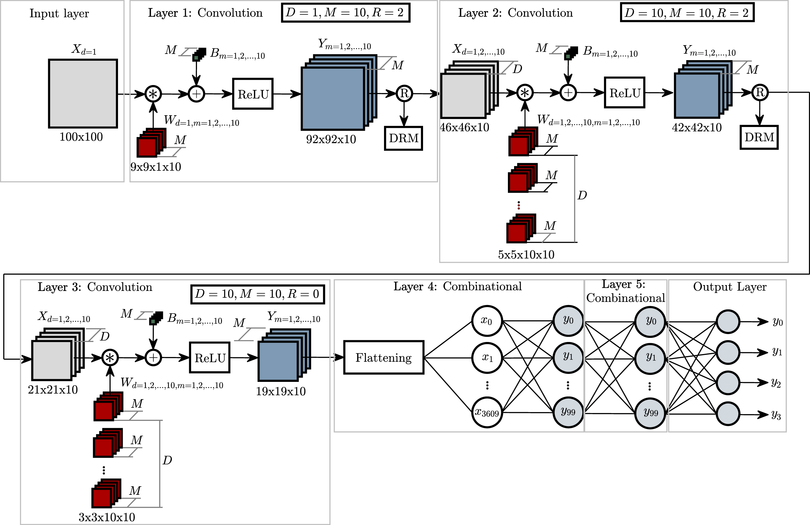
Proposed CNN to the identification algorithm.

where X_d is the input map of d ∈ D channels, W_d,m is the kernel associated with the d input channel and the m output, B_m is the bias matrix, f is the activation function, and Y_m is the m output map. The max function is used in the 2 x 2 size pool window, where the address of the maximum value is stored in the DRM vector to the CNN training process. In Fig. 2, the convolution operation is represented by an asterisk (*), the addition of the bias by a plus sign (+), and the pooling layer by an R. The activation function used in the convolution and feed-forward hidden layers is the Rectified Linear Unit function (ReLU(z) = max (0, z)) because of the property of avoiding the fading effect of the loss gradient in the training process. For the output layer, the sigmoid function described in Equation 2 is used. $sigmoid (z) = (1 + e^{- z})^{- 1}$ (2) The kernel size of the first convolutional layer is 9x9x1x10, for the second layer it is 5x5x10x10 and for the third layer it is 3x3x10x10. The fourth and fifth combinatorial layer has 100 output nodes.

The kernels size is selected by the behavior of the loss function in the training step of the CNN; the design of the net is that the first layer process the input image in big areas, the second layer in a smaller area, and the third layer process for extract details of the image. The best-obtained results are 9x9 for the first, 5x5 for the second, and 3x3 for the third. The total synaptic weights of the proposed CNN are 375,640, and the total number of neurons is 29,384.

2.2 Image creation from position signals

Two transposed vectors are multiplied to obtain an image from the motion and torque signals. The first step in the image creation is subsampling the robot position and torque signals with the Discrete Cosine Transform II (DCT-II) $C$ [29]. The DCT-II can reduce the length of a signal to an integer as described in the Equation 3; technics used in related work to subsample the signals are limited to the original signal length.

$\begin{matrix} C {(x)}_{k} = \sqrt{2 / M} \sum_{i = 1}^{M} x_{i} a \cos [\frac{π}{2 M} (2 i - 1) (k - 1)] \\ a = \frac{1}{\sqrt{1 + δ (k - 1)}}, X = C (x) \\ {X_{s_{i}} = X_{i} | \forall i \in [1, N_{s}]}, x_{s} = C^{- 1} (X_{s}) \end{matrix}$ (3) where δz is the Kronecker delta, M is the length of the original signal, N_s is the subsampled length, k is the frequency index, x_s indicates the sub-sampled signal of x, and $C^{- 1}$ is the inverse DCT-II. To estimate the velocities $\dot{q}$ and the accelerations $\ddot{q}$ of the robot, the quantized position signal $\overset{˘}{q}$ is filtered first as indicated in the Equation 4, then the expansion to the first differential term of the Taylor series of the filtered position described in the Equation 5 is used to estimate the derivatives.

${\overset{⌣}{q}}_{f} = C^{- 1} [C (\overset{⌣}{q}) e^{- λ ω^{2}}], {\overset{⌣}{τ}}_{f} = C^{- 1} [C (\overset{⌣}{τ}) e^{- λ ω^{2}}]$ (4)

$\begin{matrix} {\dot{\overset{⌣}{q}}}_{f} (k - 1) \approx \frac{1}{h} [{\overset{⌣}{q}}_{f} (k) - {\overset{⌣}{q}}_{f} (k - 1)] \\ {\ddot{\overset{⌣}{q}}}_{f} (k - 1) \approx \frac{1}{h} [{\dot{\overset{⌣}{q}}}_{f} (k) - {\dot{\overset{⌣}{q}}}_{f} (k - 1)] \end{matrix}$ (5) where $\overset{˘}{q}$ indicates the quantization of q by an ADC, ω is the frequency of the DCT-II spectrum, λ is the filtering coefficient, τ is the robot torque and h is the sampling time.

The image is created with vector ψ and vector α, as described in Fig. 3. These vectors are different for each robot, and their content is a function of the specific dynamic model of each robot. The general representation for the ψ and α is in Equation 6:

Fig. 3

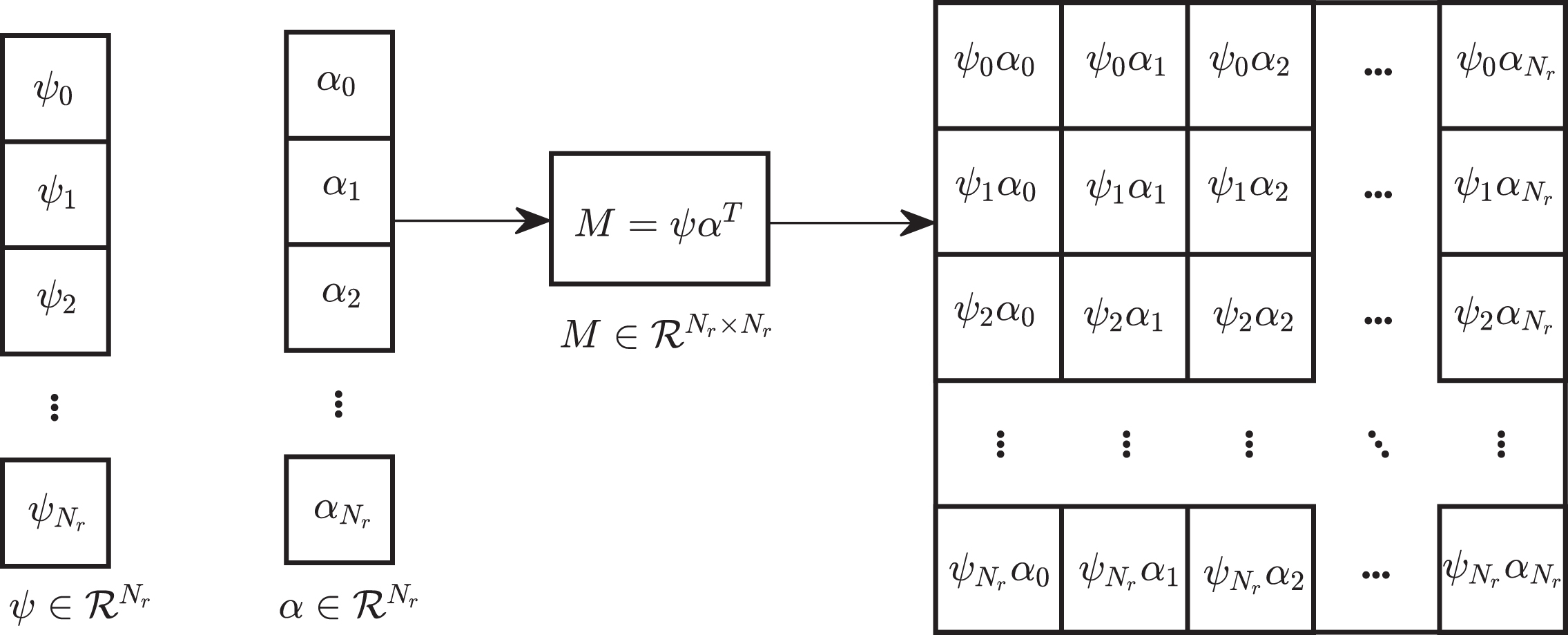
Image from signals of the feed-drive robot.

$\begin{matrix} ψ = f_{ψ} (q, \dot{q}, \ddot{q}, τ_{q}, P), α = f_{α} (q, \dot{q}, \ddot{q}, τ_{q}, P) \end{matrix}$ (6) where P are the parameters of the dynamic model.

2.3 Training of the CNN

A repository of n_sim simulations of the dynamic model $f (q, \dot{q}, \ddot{q}, P)$ is generated to train the CNN; the dynamic parameters range from 1e-3 to 1 for inertia and friction coefficients and -1 to 1 for gravity coefficients. The trajectory used to generate the training data is a sinusoidal signal of frequency a implemented by a proportional derivative position control with dynamic compensation to avoid tuning the gains for each set of parameters. The proportional k_p and derivative k_v gains are proportional to the inertia parameters of the robot to be identified [30]; I_T represents inertia for each DOF of the robot, and the rise time t_r is set to 0.1 ms as shown in the Equation 7:

$\begin{matrix} τ_{c_{q}} = k_{p} (q_{d} - q) - k_{v} \dot{q} + f (q, \dot{q}, \ddot{q}, P) \\ q_{d} = 2 π \sin (a t), k_{p} = \frac{I_{T}}{4} {(\frac{10}{t_{r}})}^{2}, k_{v} = \sqrt{4 I_{T} k_{p}} \end{matrix}$ (7)

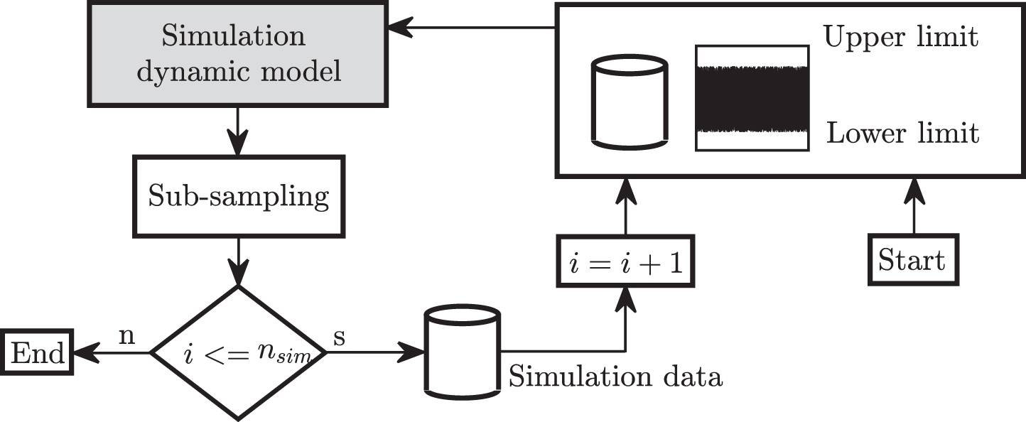
The training data in Fig. 4 is subsampled with the Equation 3. The motion and torque signals of the simulations are taken to generate the images. The training process of the CNN uses two types of images; the Mp images constructed with the dynamic parameters that match with position and torque signals, and the Mn images that use random parameters, as illustrated in Fig. 5. The sig2im function generates the vectors ψ and α to perform the transpose multiplication and obtain the image.

Fig. 4

Simulation to create the data to train the CNN.

Fig. 5

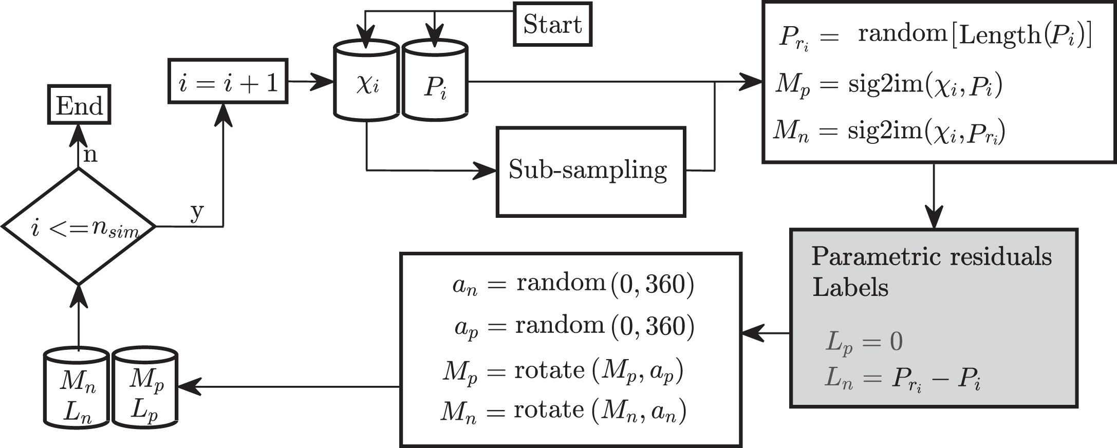
Training image generation.

Half of the image repository is Mp, and the other half is Mn. The labels put in Mp images are zero because of the zero parameter error. The labels of Mn images are the subtraction of the simulation parameters and the randomly selected parameters. Each image is rotated in four possible random orientations (0°, 90°, 180°, 270°) to avoid CNN memorization (see Fig. 5).

The CNN training process uses the propagation error algorithm with the loss function $L = \frac{1}{2} (y_{d} - y)$ ; y_d is the real parameters obtained from the image label, and y is the CNN outputs. The training coefficient η is modified for each robot.

2.4 Evaluation metric

The evaluation metric analyzes the similarity between two signals in the time and DCT-II frequency domain. The correlation is used as an evaluation metric in the related work, but the high-frequency variations are not considered. The proposed metric metr2ev is described in Equation 8:

$p_{n} (X, Y) = (1 - [\frac{| \sum_{i = 0}^{N - 1} X_{i} - \sum_{i = 0}^{N - 1} Y_{i} |}{\sum_{i = 0}^{N - 1} (| X_{i} | + | Y_{i} |)}]) (1 - [\frac{\sum_{i = 0}^{N} | X_{c n_{i}} - Y_{c n_{i}} |}{\sum_{i = 0}^{N - 1} (| X_{c n_{i}} | + | Y_{c n_{i}} |)}]) m e t r 2 e v = 100 [p_{n} {(X, Y)}^{ϵ}] X_{c n} = C_{n} (X), Y_{c n} = C_{n} (Y)$ (8) where ε is set in 0.4 units, X_cn, Y_cn is the normalized DCT-II spectrum of X, Y, respectively, and i is the frequency sample for X_cn, Y_cn, and the time sample for X, Y. To evaluate the results of the parameter identification, the X signal is the real input torque and the Y signal is the torque determined by the identified parameters.

2.5 Identification algorithm

The algorithm shown in pseudocode 1 identifies the parameters of a robot introducing the robot position and torque signals, its dynamic model, and the CNN trained parameters. In lines 1 and 2, the derivative is estimated by the function low2dev where first the filter shown in the Equation 4 is applied, and then the Equation 5 is applied to estimate speed and acceleration. Lines 3 and 4 show the filtering of the position and torque obtained from the robot’s measurement system; all filters applied in the algorithm use the same λ parameters. In line 5, the filtered signals are subsampled by the dct2sub function described in the Equation 3.

Algorithm 1

Parametric Identification

Input:   Robot position $\overset{˘}{q}$ , torque $\overset{˘}{τ}$ , dynamic model $f (x = q, \dot{q}, \ddot{q}, P)$ , sample time h and trained CNN parameters W

  1:    ${\dot{\overset{˘}{q}}}_{f} \leftarrow$ low2dev $(\overset{˘}{q}, h, λ)$

  2:    ${\ddot{\overset{˘}{q}}}_{f} \leftarrow$ low2dev $({\dot{\overset{˘}{q}}}_{f}, h, λ)$

  3:    ${\overset{˘}{τ}}_{q_{f}} \leftarrow$ low $({\overset{˘}{τ}}_{q}, λ)$

  4:    ${\overset{˘}{q}}_{f} \leftarrow$ low $(\overset{˘}{q}, λ)$

  5:    ${{\overset{˘}{q}}_{fs}, {\dot{\overset{˘}{q}}}_{fs}, {\ddot{\overset{˘}{q}}}_{fs}, {\overset{˘}{τ}}_{fs}} \leftarrow$ dct2sub ${{\overset{˘}{q}}_{f}, {\dot{\overset{˘}{q}}}_{f}, {\ddot{\overset{˘}{q}}}_{f}, {\overset{˘}{τ}}_{f}}$

  6:   v ← 0

  7:   P_out←alloc ( n_P parameters)

  8:   whilev < v_sandP_out physically not valid do

  9:         P_out← random(n_P numbers)

10:           $ψ \leftarrow f_{ψ} ({\overset{⌣}{q}}_{f s}, {\dot{\overset{⌣}{q}}}_{f s}, {\ddot{\overset{⌣}{q}}}_{f s}, P_{o u t})$

11:           $α \leftarrow f_{α} ({\overset{⌣}{q}}_{f s}, {\dot{\overset{⌣}{q}}}_{f s}, {\ddot{\overset{⌣}{q}}}_{f s}, P_{o u t})$

12:          M ← ψα^T

13:          M← normalize(M)

14:          y← CNN(W, M)

15:           $P_{r} \leftarrow - \ln [\frac{(1 - y)}{y}]$

16:          P_out ← P_out - P_r

17:           $x \leftarrow {\overset{˘}{q}, {\dot{\overset{˘}{q}}}_{f}, {\ddot{\overset{˘}{q}}}_{f}}$

18:          τ_out ← f (x, P_out)

19:          v← metr2ev $(τ_{out}, \overset{˘}{τ})$

20:    $P_{out} \leftarrow P_{out} \frac{max (\overset{˘}{τ})}{max (τ_{out})}$

Output: Dynamic parameters P_out

Parametric Identification
Input: Robot position $\overset{˘}{q}$ , torque $\overset{˘}{τ}$ , dynamic model $f (x = q, \dot{q}, \ddot{q}, P)$ , sample time h and trained CNN parameters W
1: ${\dot{\overset{˘}{q}}}_{f} \leftarrow$ low2dev $(\overset{˘}{q}, h, λ)$
2: ${\ddot{\overset{˘}{q}}}_{f} \leftarrow$ low2dev $({\dot{\overset{˘}{q}}}_{f}, h, λ)$
3: ${\overset{˘}{τ}}_{q_{f}} \leftarrow$ low $({\overset{˘}{τ}}_{q}, λ)$
4: ${\overset{˘}{q}}_{f} \leftarrow$ low $(\overset{˘}{q}, λ)$
5: ${{\overset{˘}{q}}_{fs}, {\dot{\overset{˘}{q}}}_{fs}, {\ddot{\overset{˘}{q}}}_{fs}, {\overset{˘}{τ}}_{fs}} \leftarrow$ dct2sub ${{\overset{˘}{q}}_{f}, {\dot{\overset{˘}{q}}}_{f}, {\ddot{\overset{˘}{q}}}_{f}, {\overset{˘}{τ}}_{f}}$
6: v ← 0
7: P_out←alloc ( n_P parameters)
8: whilev < v_sandP_out physically not valid do
9: P_out← random(n_P numbers)
10: $ψ \leftarrow f_{ψ} ({\overset{⌣}{q}}_{f s}, {\dot{\overset{⌣}{q}}}_{f s}, {\ddot{\overset{⌣}{q}}}_{f s}, P_{o u t})$
11: $α \leftarrow f_{α} ({\overset{⌣}{q}}_{f s}, {\dot{\overset{⌣}{q}}}_{f s}, {\ddot{\overset{⌣}{q}}}_{f s}, P_{o u t})$
12: M ← ψα^T
13: M← normalize(M)
14: y← CNN(W, M)
15: $P_{r} \leftarrow - \ln [\frac{(1 - y)}{y}]$
16: P_out ← P_out - P_r
17: $x \leftarrow {\overset{˘}{q}, {\dot{\overset{˘}{q}}}_{f}, {\ddot{\overset{˘}{q}}}_{f}}$
18: τ_out ← f (x, P_out)
19: v← metr2ev $(τ_{out}, \overset{˘}{τ})$
20: $P_{out} \leftarrow P_{out} \frac{max (\overset{˘}{τ})}{max (τ_{out})}$
Output: Dynamic parameters P_out

In line 6, the variable v for the evaluation metric shown in the Equation 8 is initialized with zeros. The parameters are initialized by assigning n_p numbers, as shown in line 7. The while loop of line 9 runs until the variable v exceeds a threshold v_s and the identified parameters P_out are physically possible; the coefficients of inertia and friction must be positive, while the gravity coefficients can have positive or negative values. Within the while loop, n_P random numbers of range 0 to 1 are assigned to P_out. The vectors ψ and α are determined using the equations ref eq6 as shown in lines 10 and 11 to create the M image of line 12. In line 13, M is normalized to a range of 0 to 1, and it is introduced to the CNN in line 14.

Because the sigmoid function is used in the CNN output layer, in line 15, the parametric residual P_r is recovered by applying the inverse sigmoid function. In line 16, the identified parameters are obtained by subtracting P_r from P_out. The torque determined by P_out is constructed with the dynamic model f (x, P) and the set of signals x, as shown in lines 17 and 18. The evaluation metric is applied to the τ_out and the input torque to determine their similarity. Finally, P_out is denormalized in line 20 to identify any value inside and outside the range -1 to 1.

3 Case of study: Feed-drive robot

3.1 Description of the robot

The robot to be identified with the proposed methodology is a 2-DOF feed drive robot [31]. The robot uses two DC motors for each degree of freedom coupled to a 131.25:1 gearbox. Two incremental encoders with a resolution of 8400 counts per revolution of the output shaft reducer are implemented to measure the position. The maximum velocity for x-motor v_mx and z-motor v_mz are 10x10³ rpm. Both gearboxes are connected to an endless screw that is part of the ball screw drive mechanism used to convert axial movement into linear movement with a 2mm/π rad reduction. Figure 6 shows the connection between the x-axis nut and the z-axis support table where it has a rectified linear rail to support the base of the floor.

Fig. 6

Feed-drive robot of two degrees of freedom.

The robot embedded electronics shown in Fig. 7 consist of a field-programmable gate array (FPGA) with a microprocessor connected to the peripheral controller firmware required to drive the robot’s DC motors, process the encoder position signal, and implement the control system to set the desired trajectory. The acquisition of the robot signals is made through Wi-Fi communication between the FPGA system and an external computer in a sampling time of 2.5ms. The programming of the microprocessor and the data acquisition is made by a software design in Labview ©.

Fig. 7

General diagram of the embedded electronics.

The schematic diagram of the feed-drive robot is shown in Fig. 8. The output shafts of the gearboxes, couplings, and endless screws are connected in series to facilitate the determination of the dynamic model. The gearboxes and nuts of the ball screw mechanism are placed as a reduction constant, a spring, and a damper, shown in the Fig. 8. The couplings and supports of the robot are represented by springs and dampers.

Fig. 8

Schematic diagram of the feed-drive robot. The torsional stiffness κ_{mg
_x} and κ_{mg
_z} are represented by the gears, and torsional friction β_{mg
_x} and β_{mg
_z} are between the tooth of the gears. For the torsional stiffness κ_{gs
_x} and κ_{gs
_z}, it is used a connection bar, and for the torsional friction β_{gs
_x} and β_{gs
_z}, it is used a hollow bar.

3.2 Modeling of the robot

The dynamic model of the robot considers that the sum of the external forces and reaction forces is equal to the mass by their acceleration. In the case of rotational joints, forces are replaced by torques and mass by a moment of inertia: $\sum_{i = 0}^{n} F_{i} = m_{i} a_{i}$ , $\sum_{i = 0}^{n} τ_{i} = I_{i} α_{i}$ .

The model equations for the x and z axes are described in the Equation 1:

$\begin{matrix} {\ddot{θ} = A}_{x}^{- 1} [τ_{x} - B_{x} \dot{θ} - C_{x} sign (\dot{θ}) - K_{x} θ] \\ θ = {[θ_{m}, θ_{g}, θ_{s}, x_{l}, x_{s}, x_{A}]}^{T} \\ τ_{x} = diag {τ_{m_{x}}, 0, 0, 0, 0, 0} \end{matrix}$

$\begin{matrix} \ddot{ϕ} = A $_{z}^{- 1} [τ_{z} - B_{z} \dot{ϕ} - C_{z} s i g n (\dot{ϕ}) - K_{z} $ ϕ - g] \\ ϕ = {[ϕ_{m}, ϕ_{g}, ϕ_{s}, z_{l}, z_{s}]}^{T} \\ τ_{z} = diag {τ_{m_{z}} - m_{l_{z}} $ g, 0, 0, 0, 0} \\ A_{x} = diag {J_{m_{x}}, J_{g_{x}}, J_{s_{x}}, m_{l_{x}}, m_{s_{x}}, m_{A_{x}} + m_{s_{z}} + m_{l_{z}}} \\ A_{z} = diag {J_{m_{z}}, J_{g_{z}}, J_{s_{z}}, m_{l_{z}}, m_{s_{z}}} \\ B_{1_{x}} = [β_{m_{x}} + β_{m g_{x}}, - r_{x} β_{m g_{x}}, 0, 0, 0, 0] \\ B_{2_{x}} = [- r_{x} β_{m g_{x}}, β_{g_{x}} + r_{x}^{2} β_{m g_{x}} + β_{g s_{x}}, - β_{g s_{x}}, 0, 0, 0] \end{matrix}$ $\begin{matrix} B_{3_{x}} = [0, - β_{g s_{x}}, β_{s_{x}} + β_{g s_{x}} + β_{s l_{x}}, - n_{x} β_{s l_{x}}, 0, 0] \\ B_{4_{x}} = [0, 0, - n_{x} β_{s l_{x}}, n_{x}^{2} β_{s l_{x}} + b_{l s_{x}} + b_{l A}, - b_{l s_{x}}, - b_{l A}] \\ B_{5_{x}} = [0, 0, 0, - b_{l s_{x}}, b_{l s_{x}} + b_{s_{x}}, 0] \\ B_{6_{x}} = [0, 0, 0, - b_{l A}, b_{l A}, 0] \\ B_{x} = {[B_{1_{x}}^{T}, B_{2_{x}}^{T}, B_{3_{x}}^{T}, B_{4_{x}}^{T}, B_{5_{x}}^{T}, B_{6_{x}}^{T}]}^{T} \end{matrix}$ $\begin{matrix} B_{1_{z}} = [β_{m_{z}} + β_{m g_{z}}, - r_{z} β_{m g_{z}}, 0, 0, 0] \\ B_{2_{z}} = [- r_{z} β_{m g_{z}}, β_{g_{z}} + r_{z}^{2} β_{m g_{z}} + β_{g s_{z}}, - β_{g s_{z}}, 0, 0] \\ B_{3_{z}} = [0, - β_{g s_{z}}, β_{s_{z}} + β_{g s_{z}} + β_{s l_{z}}, - n_{z} β_{s l_{z}}, 0] \\ B_{4_{z}} = [0, 0, - n_{z} β_{s l_{z}}, n_{z}^{2} β_{s l_{z}} + b_{l s_{z}}, - b_{l s_{z}}] \\ B_{5_{z}} = [0, 0, 0, - b_{l s_{z}}, b_{l s_{z}} + b_{s_{z}}] \\ B_{z} = {[B_{1_{z}}^{T}, B_{2_{z}}^{T}, B_{3_{z}}^{T}, B_{4_{z}}^{T}, B_{5_{z}}^{T}]}^{T} \\ C_{x} = diag {γ_{m_{x}}, γ_{g_{x}}, γ_{s_{x}}, c_{l_{x}}, c_{s_{x}}, c_{A_{x}}} \\ C_{z} = diag {γ_{m_{z}}, γ_{g_{z}}, γ_{s_{z}}, c_{l_{z}}, c_{s_{z}}} \end{matrix}$ (9)

where the angular position of the motors θ_m, φ_m, the output shaft of the gearboxes θ_g, φ_g, the endless screws θ_s, φ_s and, the linear displacements x_l, x_s, x_A, z_l, z_s are in the vectors θ and φ. The equations of the feed-drive begin with the motors that are modeled with inertia parameters J_mx andJ_mz, and viscous frictionβ_mx and β_mz; the torque applied is by a PWM signal of the embedded system that corresponds with the motors torque [31]. The gearboxes are modeled with the total axial stiffness, κ_mgx, and κ_mgz, of the gears. The viscosity between gears teeth are β_mgx andβ_mgz coefficients;β_gx and β_gz model the lubricant of the gearboxes. The connection between the output shaft of the gearboxes is modeled with axial stiffnessκ_gsx andκ_gsz coefficients. The model for these connections includes the viscosity frictionβ_gsx and β_gsz between the endless screws represented byθ_s and φ_s. The axial motion is converted to linear motion with a nut;κ_slx andκ_slz model their stiffness and viscosity, β_slx andβ_slz. The mass m_lx and m_lz represent the tables where the nut is attached. The mass m_A corresponds with the support for the z-axis. Finally, the tables move in the bases supported by m_sx andm_sx, in which stiffness and viscosity are defined by k_sx, k_sz,b_sx, andb_sz.

\begin{matrix} K_{1_{x}} = [κ_{m g_{x}}, - r_{x} κ_{m g_{x}}, 0, 0, 0, 0] \\ K_{2_{x}} = [- r_{x} κ_{m g_{x}}, r_{x}^{2} κ_{m g_{x}} + κ_{g s_{x}}, - κ_{g s_{x}}, 0, 0, 0] \\ K_{3_{x}} = [0, - κ_{g s_{x}}, κ_{g s_{x}} + κ_{s l_{x}}, - n_{x} κ_{s l_{x}}, 0, 0] \\ K_{4_{x}} = [0, 0, - n_{x} κ_{s l_{x}}, n_{x}^{2} κ_{s l_{x}} + k_{l A}, 0, - k_{l A}] \\ K_{5_{x}} = [0, 0, 0, 0, k_{s_{x}}, 0] \\ K_{6_{x}} = [0, 0, 0, - k_{l A}, 0, k_{l A}] \end{matrix}

\begin{matrix} K_{x} = {[K_{1_{x}}^{T}, K_{2_{x}}^{T}, K_{3_{x}}^{T}, K_{4_{x}}^{T}, K_{5_{x}}^{T}, K_{6_{x}}^{T}]}^{T} \\ K_{1_{z}} = [κ_{m g_{z}}, - r_{z} κ_{m g_{z}}, 0, 0, 0] \\ K_{2_{z}} = [- r_{z} κ_{m g_{z}}, r_{z}^{2} κ_{m g_{z}} + κ_{g s_{z}}, - κ_{g s_{z}}, 0, 0] \\ K_{3_{z}} = [0, - κ_{g s_{z}}, κ_{g s_{z}} + κ_{s l_{z}}, - n_{x} κ_{s l_{z}}, 0] \\ K_{4_{z}} = [0, 0, - n_{z} κ_{s l_{z}}, n_{z}^{2} κ_{s l_{z}}, 0,] \\ K_{5_{z}} = [0, 0, 0, 0, k_{s_{z}}] \\ K_{z} = {[K_{1_{z}}^{T}, K_{2_{z}}^{T}, K_{3_{z}}^{T}, K_{4_{z}}^{T}, K_{5_{z}}^{T}]}^{T} \end{matrix}

(10)

The mass parameters ( $m_{l_{x}}, m_{s_{x}}, m_{A_{x}}, m_{l_{z}}, m_{s_{z}}$ ) and inertia moments ( $J_{m_{x}}, J_{g_{x}}, J_{s_{x}}, J_{m_{z}}, J_{g_{z}} J_{s_{z}}$ ) are in the A^zmatrices whose components are on the diagonal as shown in Equation 9. The viscose friction parameters of the motors (β_{m
_x}, β_{m
_z}), the gearboxes (β_{g
_x}, β_{g
_z}), endless screws (β_{s
_x}, β_{s
_z}), linear supports (b_{s
_x}, b_{s
_z}, b_{A
_x}), thez-axis table support (b_{l
_x}), and end effector displacement (b_{l
_z}) are grouped in theB_x and B_z matrices, while the Coulomb friction of motors, gearboxes, endless screw (γ_{m
_x}, γ_{g
_x}, γ_{s
_x}, γ_{m
_z}, γ_{g
_z} and linear displacements (c_{l
_x}, c_{s
_x}, c_{A
_x}, c_{l
_z}, c_{s
_z}) are in the diagonal matrices C_x andC_z as shown in Equation 9 and 13. The gravitational vector isg = [0, 0, 0, 0, m_{l
_z}g], and the number of variables N_x for thex-axis is six due to the massm_A and, for the z-axisN_z is five.

\begin{matrix} I_{x} = r_{x} J_{m_{x}} + J_{g_{x}} + J_{s_{x}} + \frac{1}{n_{x}} (m_{l_{x}} + m_{A} + m_{s_{z}} + \\ m_{l_{z}}) \\ I_{z} = r_{z} J_{m_{z}} + J_{g_{z}} + J_{s_{z}} + \frac{1}{n_{z}} m_{l_{z}} \\ b_{x} = r_{x} β_{m_{x}} + β_{g_{x}} + β_{s_{x}} + \frac{1}{n_{x}} b_{l_{x}} \\ b_{z} = r_{z} β_{m_{z}} + β_{g_{z}} + β_{s_{z}} + \frac{1}{n_{z}} b_{l_{z}} \\ c_{x} = r_{x} γ_{m_{x}} + γ_{g_{x}} + γ_{s_{x}} + \frac{1}{n_{x}} c_{l_{x}} \end{matrix}

\begin{matrix} c_{z} = r_{z} γ_{m_{z}} + γ_{g_{z}} + γ_{s_{z}} + \frac{1}{n_{z}} c_{l_{z}} \\ g_{x} = 0, g_{z} = \frac{1}{n_{z}} m_{l_{z}} g \end{matrix}

(11)

\begin{matrix} \ddot{θ} = \frac{1}{I_{x}} [τ_{x} - b_{x} \dot{θ} - c_{x} sign (\dot{θ}) - g_{x}] \\ \ddot{φ} = \frac{1}{I_{z}} [τ_{z} - b_{z} \dot{φ} - c_{z} sign (\dot{φ}) - g_{z}] \end{matrix}

(12)

The mechanical couplings of motors-gearboxes (κ_{mg
_x}, κ_{mg
_z}), gearboxes-endless screws (κ_{gs
_x}, κ_{gs
_z}), screws-nuts (κ_{sl
_x}, κ_{sl
_z}) and mechanical supports (k_{s
_x}, k_{s
_z}, k_{A
_x}) are in the matrices K_x andK_z. The reduction of the gearboxes are inr_x = 131.25 andr_z = 131.25, while the nut reduction are inn_x = 2/π mm/rad andn_z = 2/π mm/rad. To group the dynamic parameters of equations 10, the deformations of the mechanical connections are considered to be less than the encoder resolution; for axial connections Δa = 1.1905e-04 [rad], while for linear displacements ΔL = 4.7619e-07 [m]. These deformation considerations made the connection term equal to zero K_xθ → 0, K_zφ → 0}. Thus, eight parameters can be determined to obtain a reduced version of equations 9 where τ_x = r_xτ_{m
_x}, τ_z = r_zτ_{m
_z}. Variables θ and φ are taken from the output shaft of both gearboxes. With the set of equations shown in 12, ψ and α vectors are constructed with the eight parameters as Equation 13 shown. For this specific case study, the α vector is set as the torque. The main idea of the image construction for the feed drive robot is that when the identified parameters match the torque signals, the M image contains an approximation of the square value of the torque. It is important to note that the ψ and α vectors are not limited to the form presented in this case study.

\begin{matrix} ψ_{θ} = 2 {\overset{˘}{τ}}_{{xf}_{s}} - {\hat{I}}_{x} {\ddot{\overset{˘}{θ}}}_{f_{s}} - {\hat{b}}_{x} {\dot{\overset{˘}{θ}}}_{f_{s}} - {\hat{c}}_{x} sign ({\dot{\overset{˘}{θ}}}_{f_{s}}) - {\hat{g}}_{x} \\ ψ_{φ} = 2 {\overset{˘}{τ}}_{{zf}_{s}} - {\hat{I}}_{z} {\ddot{\overset{˘}{φ}}}_{f_{s}} - {\hat{b}}_{z} {\dot{\overset{˘}{φ}}}_{f_{s}} - {\hat{c}}_{z} sign ({\dot{\overset{˘}{φ}}}_{f_{s}}) - {\hat{g}}_{z} \\ α_{θ} = {\overset{˘}{τ}}_{{xf}_{s}}, α_{φ} = {\overset{˘}{τ}}_{{zf}_{s}} \end{matrix}

(13)

The verification of the algorithm uses five simulations of the 12 determined by the classic fourth-order Runge-Kutta ordinary differential equation solver. For this case study, the sinusoidal trajectory frequency is set at 0.2875 rad/s. The FPGA contains a programmed trajectory follow for the feed-drive 2-DOF robot. For the x-axis, the trajectory is θ_d = 2π sin(0.2875t), and for the z-axis is φ_d = 2π cos(0.2875t).

Data acquisition from the feed-drive robot is implemented via a wireless interface in LabView 2015 © . The raw data is transferred from the FPGA board to a personal computer to be processed by the identification algorithm. The proposed algorithm was implemented in Matlab R2017b © with the optimized convolution in two dimensions function conv2 and the functions to handle an NVIDIA graphics unit © . The data generation, CNN training, and the algorithm run on a personal computer.

4 Results

4.1 Training of the CNN

The computer used for the parameter identification algorithm has a GTX-1060© GPU with an Intel i7-8th© processor. The computational cost is determined experimentally for convolution layers 1 (100x100 input map with 9x9 kernel), 2 (46x46 input map with 5x5 kernel), and 3 (21x21 input map with 3x3 kernel). Figure 9 shows the For Loop Convolution (FLC) runtime, which is the direct implementation of the Equation 1, the Optimized Processor Convolution (OPC) of Matlab © and the solved convolution by the GPU. All times in this figure are for a single input map and convolution kernel only. For layers 4, 5, and 6, the lowest computational cost is obtained using the processor. CNN’s time cost is approximately 3.3426 ms.

Fig. 9

Computational cost of the layers 1, 2 and 3.

The generated training set described in Fig. 5 is divided into train set and test set to avoid over-learning of the CNN. Figure 10 shows the evolution of the loss function for both training tests with a learning rate set to η = 0.14 units. The loss function is close to zero in the first 0.1 × 10⁶ iterations due to the range of the parameters residuals. However, the sigmoid function tends to minimize the residuals of the parameters, and the error evaluated with the proposed metric is greater than the loss training function.

Fig. 10

Loss function of the CNN training process.

The normalized Fourier frequency spectrum of the 210 trained kernels is shown in Fig. 11. The characteristics of the Mimage are extracted using the shape of each kernel spectrum to determine the parameters with the feed-forward part of the CNN. It is observed that the kernels are different from each other, and each kernel in combination with the activation function determines the parameters of the Equation 18.

Fig. 11

Frequency spectrum of the kernels of the layers 1, 2 and 3 using the Fourier transform.

Figure 12 shows four M_p and M_n with their respective labels. The M_p images for the Equation 12 have an approximation of the square value of the torque, but the M_n images do not match the square torque. When the vectors ψ and α contain parameters that are not correct, the resultant image is unbalance.

Fig. 12

Normalized images M_p and M_n from the training set.

4.2 Simulation results

The parameters used in the five simulations are described in Table 1. The simulations S4 and S5 have parameters outside the range -1 to 1 to verify the denormalization step of the algorithm. Table 2 describes the results of the evaluation metric along with the execution time of the identification algorithm and the identified parameters.

Table 1
Dynamic parameters used to the five simulations

P S1 S2 S3 S4 S5

I kg·m² 0.05 0.1 0.1 3 50

b kg · m² · s 0.4 0.4 0.8 40 60

c N·m 0.07 0.1 0.1 7 40

g N·m 0 0.05 0.4 2 4

P	S1	S2	S3	S4	S5
I kg·m²	0.05	0.1	0.1	3	50
b kg · m² · s	0.4	0.4	0.8	40	60
c N·m	0.07	0.1	0.1	7	40
g N·m	0	0.05	0.4	2	4

Fig. 13

Comparison between torque simulations and torque obtained by the identified parameters.

Table 2

Identified dynamic parameters with evaluation metric and execution time

$\hat{P}$	S1	S2	S3	S4	S5
$\hat{I} kg \cdot m^{2}$	0.0517	0.0891	0.1035	3	51.4989
$\hat{b} kg \cdot m^{2} \cdot s$	0.3988	0.3858	0.8058	39.3516	62.2023
$\hat{c} N \cdot m$	0.0668	0.1288	0.087	7.5399	35.85
$\hat{g} N \cdot m$	0.0002	0.045	0.4024	2.61	4.1202
metr2ev	99.82%	98.52%	99.61%	99.23%	99.16%
t _exe s	3.92	0.017	0.0626	0.0136	0.0476

The evaluation with metr2ev for the simulation signals has values that exceed 98% similarity. The execution time tends to be less than one second, except in simulation 1, where the execution time is less than 4 seconds. With the denormalization technique implemented in the proposed algorithm, it is observed that although the training data were created with parameters only in the range of -1 to 1, the algorithm can identify parameters outside this range.

4.3 Identification results to the study case: Feed-drive robot

The trajectory made by the feed-drive robot is shown in Fig. 14 where for both axes, the position, torque, and estimations of velocity and acceleration, are cut to adjust to the sinusoidal training trajectory. Multiplying θ and φ for the reduction of the screwball parameters n_x and n_y, the position of the end effector is obtained as shown in the Fig. 15 where the black arrow shows the direction of the trajectory.

Fig. 14

Signals of the position, velocities estimations and accelerations estimation for both axis of the feed-drive robot.

Fig. 15

Trajectory of 2 dimensions of the feed-drive robot.

Table 3 shows the identification results of the parameters shown in Equation 18 of the feed-drive robot with the evaluation metric and the algorithm execution time. For both axes of the feeding robot, the metr2ev is above 90% , and the execution time is less than 1 second.

Table 3

Identified dynamic parameters with evaluation metric and execution time

$\hat{P}$	x	z
$\hat{I} kg \cdot m^{2}$	0.0041	0.0089
$\hat{b} kg \cdot m^{2} \cdot s$	0.2302	0.2970
$\hat{c} N \cdot m$	0.0817	0.0167
$\hat{g} N \cdot m$	0.0001	0.0092
metr2ev	91.96%	90.31%
t _exes	0.8126	0.2142

Figure 16 shows the comparison between the torques of the feed-drive robot and the torque obtained by the identified parameters. For the axis x the shape of the real torque is close to the torque built with the identified parameters. The error shown in the black dashed line is more significant at zero-torque transitions than the other parts. In the real torque, the z is close, but the metr2ev is lower than the x axis. The torque error for this axis is greater than that of the x axis, and the error is more significant in the same transition region. The gravitational coefficient of the x axis is close to zero. Meanwhile, the z axis has a m_{l
_z} mass of 1.4731 kg determined by the Equation 14.

Fig. 16

Comparison between feed-drive torques and torque obtained by the identified parameters.

The proposed evaluation metric metr2ev considers the slight variations of the signals to be compared. On the x-axis, even though the real torque is too close to the identified parameter torque, the similarity percentage does not exceed 92 % because there are high-frequency differences with small amplitude of the DCT-II metr2ev part in the zero-crossing region: It is considered that the error torque in the x-axis is modeled as a pulse of around 0.2 seconds at zero cross-region, as shown Fig. 16. By the Fourier theory, it is found that the estimated frequency of the impulse is 10Hz [32]. The maximum frequency of the feed-drive x-axis robot is $f_{m x} = v_{m x} / 60 r_{x} = 1.26 H z$ . As a result, the error torque frequency is considered a high frequency at zero cross-region.

The characteristics of the proposed evaluation metric for electronic signals make it ideal for comparison because it considers the frequency spectrum in the DCT-II transform.

5 Discussion

Optimizing a trajectory to identify dynamic robot parameters takes time because each new trajectory needs to be tested on the real robot. With the proposed methodology, trajectory optimization is not necessary, and the processing time is reduced. The preprocessing technique applied to the input data can subsample the signals to any integer value length with the DCT-II; this frequency transformation contains the most significant information in the first frequency bins.

The transformation of signals into an image helps in the training of the proposed CNN. Other transformation methods such as the time-frequency spectrum are reported. However, the technique used in this work does not require the frequency spectrum and has the necessary information in a simple way to be processed by the CNN to obtain the dynamic parameters. The proposed CNN-based algorithm works with estimates made by position measurements rather than real velocity and acceleration measurements. The CNN can generalize the input information to identify parameters not included in the training data set.

The proposed algorithm has a short running time. Once the CNN has been trained with one type of robot, it can be applied to any real robot with the same dynamic model, which makes it helpful in identifying many robots. The future work of this investigation is to extend the dynamic model to increase the similarity with the proposed metric.

6 Conclusions

In this paper, has been presented an algorithm for parameter identification based on a convolutional neural network. The feed-drive robot is used to test the proposed algorithm. The parameters extraction with a CNN and the creation of the image are the novelty parts of this work. For the image creation with robot motion signals, the proposed transformation technique puts enough information into a small image to determine the parameters quickly. The proposed methodology does not require the optimization step of a trajectory performed by a robot. Therefore, once the CNN is trained with the dynamic model of a specific type of robot, the algorithm can identify the parameters of any robot that the same model determines as the one used to train the CNN.

Unlike correlation, the most used metric in parameter identification papers, the proposed metric analyzes the information in time and frequency. This characteristic makes it ideal for comparing similarities of electronic signals such as torque measurements. The results show that, for the five simulations, the algorithm obtained a similarity greater than 98% because the simulated model was the same that was used for the CNN training. The results of the feed-drive identification show that the similarity exceeds 90% . The parameter identification for this robot contributes to validate the dynamic model of eight parameters where both estimated torque signals are close to the experimental torque signals. The results presented in this paper show that the proposed methodology works in the identification of dynamic parameters. Consequently, the future work will be the application of the proposed algorithm to identify other types of robots used commonly in the industry and investigations.

References

You

, Qiao

, Xu

and Liu

, Low-Speed Control of Heavy-LoadTransfer Robot with Long Telescopic Boom Based on Stribeck FrictionModel, Mathematical Problems in Engineering2012 (2012), 1–13.

Guo

, Zhong

and Zhou

, Multisensor Data-Fusion-Based Approachto Airspeed Measurement Fault Detection for Unmanned AerialVehicles, IEEE Transactions on Instrumentation and Measurement67(2) (2018), 317–327.

Jin

and Gans

, Parameter identification for industrial robotswith a fast and robust trajectory design approach, Robotics andComputer-Integrated Manufacturing31 (2015), 21–29.

Katsumata

, Navarro

, Bonnet

, Fraisse

, Crosnier

and Venture

, Optimal exciting motion for fast robot identification, Application to Contact Painting tasks with estimated externalforces, Robotics and Autonomous Systems113 (2019), 149–159.

, Zhang

, Hu

, Wang

, Chen

and Chen

, A dynamicparameter identification method of industrial robots consideringjoint elasticity, International Journal of Advanced RoboticSystems16(1) (2019), 1–11.

Huynh

H.N.

, Assadi

, Rivière-Lorphèvre

, Verlindenand

and Ahmadi

, Modelling the dynamics of industrial robots formilling operations, Robotics and Computer-IntegratedManufacturing61 (2020), 1–16.

Han

, Wu

, Liu

and Xiong

, An iterative Approach forAccurate Dynamic Model Identification of Industrial Robots, IEEE Transactions on Robotics36(5) (2020), 1577–1594.

Jiang

, Jiang

, Cao

, Hua

, Wu

, Ding

and Chen

, Atypical dynamic parameter identification method of 6-degreeof freedom industrial robot, Proceedings of the Institution of Mechanical Engineers, Part I: Journal of Systems and Control Engineering231(9) (2017), 740–752.

Cao

, Gan

and Dai

, Model-based sensorless robot collision detection under model uncertainties with a fast dynamics identification, International Journal of Advanced Robotic Systems16(3) (2019), 1–15.

10.

Benimeli

, Mata

and Valero

, A comparison between direct andindirect dynamic parameter identification methods in industrial robots, Robotica24(5) (2006), 579–590.

11.

Chávez Olivares

C.A.

, Reyes-Cortés

, González-Galván

E.J.

, Mendoza-Gutiérrez

M.O.

and Bonilla-Gutiérrez

, Experimental evaluation of parameteridentification schemes on a directdrive robot, Proceedings ofthe Institution of Mechanical Engineers, Part I: Journal of Systemsand Control Engineering226(10) (2012), 1419–1431.

12.

Sousa

C.D.

and Cortesão

, Inertia Tensor Properties in Robot Dynamics Identification: A Linear Matrix Inequality Approach, IEEE ASME Transactions on Mechatronics24(1) (2019), 406–411.

13.

Liu

, Li

, Hao

, Yang

, Hu

, Xue

, Wang

and Shao

, Semiparametric Deep Learning Manipulator Inverse Dynamics ModelingMethod for Smart City and Industrial Applications, Complexity2020 (2020), 1–11.

14.

and Xiong

, Contact Force Estimation for Robot ManipulatorUsing Semiparametric Model and Disturbance Kalman Filter, IEEETransactions on Industrial Electronics65(4) (2018), 3365–3375.

15.

, Huang

, Dong

, Li

and Su

C.Y.

, Adaptive Neural NetworkControl for Robotic Manipulators With Unknown Deadzone, IEEETransactions on Cybernetics48(9) (2018), 2670–2682.

16.

Nguyen

H.N.

, Le

P.N.

and Kang

H.J.

, A new calibration method forenhancing robot position accuracy by combining a robotmodel–based identification approach and an artificial neuralnetwork–based error compensation technique, Advances inMechanical Engineering11(1) (2019), 1–11.

17.

Wang

, Shao

, Yang

and Liu

, Deep Learning Aided DynamicParameter Identification of 6-DOF Robot Manipulators, IEEEAccess8 (2020), 138102–138116.

18.

Zhao

, Zhang

, Ma

and Xiao

, System identification of thenonlinear residual errors of an industrial robot using massivemeasurements, Robotics and Computer-Integrated Manufacturing59 (2019), 104–114.

19.

, Qi

, Yang

, Sandoval

, Ferrigno

and De Momi

, Deep Neural Network Approach in Robot Tool Dynamics Identification forBilateral Teleoperation, IEEE Robotics and Automation Letters5(2) (2020), 2943–2949.

20.

Agand

, Shoorehdeli

M.A.

and Khaki-Sedigh

, Adaptive recurrentneural network with Lyapunov stability learning rules for robotdynamic terms identification, Engineering Applications ofArtificial Intelligence65 (2017), 1–11.

21.

Son

N.N.

, Anh

H.P.H.

and Chau

T.D.

, Adaptive neural model optimizedby modified differential evolution for identifying 5-DOF robotmanipulator dynamic system, Soft Computing22(3) (2018), 979–988.

22.

R.T.

and Jahanshahi

M.R.

, Deep Convolutional Neural Network forStructural Dynamic Response Estimation and System Identification, Journal of Engineering Mechanics145(1) (2019), 1–25.

23.

Ding

, Li

and Chao

, Nonlinear Friction and DynamicalIdentification for a Robot Manipulator with Improved Cuckoo Search Algorithm, Journal of Robotics2018 (2018), 1–10.

24.

Wang

, Gondokaryono

, Munawar

and Fischer

G.S.

, A Convex Optimization-Based Dynamic Model Identification Package for the daVinci Research Kit, IEEE Robotics and Automation Letters4(4) (2019), 3657–3664.

25.

, Fan

, Chen

, Ng

, Ang

M.H.

, Fang

, Zhu

and Zhao

, Dynamic Identification of the KUKA LBR iiwa Robot WithRetrieval of Physical Parameters Using Global Optimization, IEEE ACCESS8 (2020), 108018–108031.

26.

Yang

, Jiang

, He

, Na

, Li

and Xu

, Adaptive ParameterEstimation and Control Design for Robot Manipulators withFinite-Time Convergence, IEEE Transactions on IndustrialElectronics65(10) (2018), 8112–8123.

27.

, Wang

, Kuen

, Ma

, Shahroudy

, Shuai

, Liu

, Wang

, Cai

and Chen

, Recent advances in convolutionalneural networks, Pattern Recognition77 (2018), 354–377.

28.

Berzal

, Redes Neuronales & Deep Learning, 1st ed., Independently published, Granada, (2018), pp. 599–686.

29.

Oppenheim

A.V.

, Schafer

R.W.

and Buck

J.R.

, Discrete-Time Signal Processing, 2nd ed., Prentice Hall, New Jersey, (1999), pp. 594–595.

30.

Khalil

H.K.

, Nonlinear Systems Third Edition, 3rd ed., Prentice Hall, New Jersey, (2002), pp. 505–544.

31.

López-Gómez

, Vargas-Treviño

M.A.D.

, Vergara-Limon

, Vargas-Treviño

, Gutiérrez-Gutiérrez

, Palomino-Merino

A.D.

, Martínez-Solis

and Félix-Beltrán

O.G.

, Influence of PWM Torque Control Frequency inDC motors by Means of an Optimum Design Method, IEEE Access8 (2020), 80691–80706.

32.

Udal

and Kukk

, An Engineering Approach to Time-FrequencyUncertainty Criteria, ELEKTRONIKA IR ELEKTROTECHNIKA117(1) (2012), 3–8.

A novel methodology of parametric identification for robots based on a CNN

Abstract

Keywords

1 Introduction

2 Propossed methodology

3.1 Description of the robot

4.1 Training of the CNN

Table 1 Dynamic parameters used to the five simulations P S1 S2 S3 S4 S5 I kg·m2 0.05 0.1 0.1 3 50 b kg · m2 · s 0.4 0.4 0.8 40 60 c N·m 0.07 0.1 0.1 7 40 g N·m 0 0.05 0.4 2 4

6 Conclusions

References

Table 1
Dynamic parameters used to the five simulations

P S1 S2 S3 S4 S5

I kg·m² 0.05 0.1 0.1 3 50

b kg · m² · s 0.4 0.4 0.8 40 60

c N·m 0.07 0.1 0.1 7 40

g N·m 0 0.05 0.4 2 4