
Abstract
Probabilistic approaches are frequently used to describe irregular activity data to assist the design and development of devices. Unfortunately, useful estimations are not always feasible due to the large noise in the data modeled, as it occurs when estimating the sea waves potential for electricity generation. In this work we propose a simple methodology based on the use of joint probability models that allow discriminating extreme values, collected from measurements as pairs of independent points, while allowing the preservation of the essential statistics of the measurements. The outcome of the proposed methodology is an equivalent data series where large-amplitude fluctuations are suppressed and, therefore, can be used for design purposes. For the evaluation of the proposed method, we used year-long databases of hourly-collected measurements of the wave’s height and period, performed at maritime buoys located in the Gulf of Mexico. These measurements are used to obtain a fluctuations-reduced representation of the energy potential of the waves that can be useful, for instance, for the design of electric generators.
Introduction
Data analysis is of critical importance in practically all areas of knowledge to support decision-making. When the data are taken by acquisition systems and more than one variable is involved, it is common for the applied analysis to be statistical in nature. The analysis of experimental data collected at multiple locations over time leads to new and unique problems in statistical modeling and inference. Historically, time series methods have been applied to problems in the physical and environmental sciences, where information is integrated or fused in order to unify data from different sources with different contextual and conceptual representations [1]. This fact accounts for the basic engineering flavor permeating the language of time series analysis.
The field of data fusion, defined in a general way as the use of techniques that combine data from multiple sources [2], focuses on the acquisition, processing, and synergistic combination of several sources of information collected by one or more sensors to provide a better understanding of the phenomenon to be considered [3].
Many examples of areas and applications exist where the combination of information from different sources is necessary. We list only some of them for illustration as well as some of the statistical questions that might be asked about such data. In distributed detection problems [4] a multi-sensor system is used that is composed of a set of sensors placed with a certain spatial distribution. These sensors can either register the same variable at different locations or they can monitor different variables [5]. These types of measurements are common in biometric systems where expert systems are frequently used to monitor various sensors [6]. Another typical use is in the processing of radio signals from multiantenna configurations in wireless communication systems [7]; multispectral astronomical and remotely sensed images [8, 9]; in multi-frame blind image deconvolution with non-stationary blurring process [10, 11]; and, speech separation and enhancement [12, 13]. Energy estimations of renewable resources are, of course, not the exception, since one must deal with multiple, noisy meteorological parameters simultaneously [14, 15].
In this work, we propose a simple methodology based on the use of joint probability models that allow suppressing large-amplitude fluctuations of the data, caused by the extreme points, while preserving the essential statistics. More specifically, we focus on a two-dimensional situation where two independent sensors report different variables over time in the form of ordered pairs with irregular activity. The methodology proposed is general and can be extended to other scenarios of two-dimensional data fusion where large-amplitude fluctuations need to be reduced. Our proposal is illustrated for the practical case of estimating the sea wave potential. We make use of year-long databases of hourly-collected measurements of the wave’s height and period, performed at maritime buoys. As a result, we generate a new series with a significantly smaller dimension, which can be used, for example, to obtain a representation of the energy potential of the waves and, eventually, use such estimations in the design of electric generators.
The rest of the paper is organized as follows. In section 2 the detailed approach to the problem is presented, also showing a general description of the data used in this work. Section 3 describes the proposed methodology. In section 4, we show the results of the proposed methodology in an example where data obtained from marine buoys are used to obtain an estimate of the energy potential of sea waves. Finally, in Section 5 we present the conclusions.
Problem statement
To determine the energy potential of sea waves, measurements collected at maritime buoys are typically used. In our case, we had access to a database consisting of a historical record of hourly-performed measurements of several parameters including the wave’s significant height (Hm) and period (T). These parameters can be used to estimate the wave’s power by following the standard Salter-Falnes formulation. Specifically, the wave’s power density, J (W/m), can be calculated in terms of Hm and T as [16]: J = (ρg2 Hm2 T)/32π, where ρ is the density of sea water (1025 kg/m3), and g is the acceleration of gravity (9.81 m/s2). If a wave with power density J impinges on a rigid body with a single degree of freedom, the maximum power absorbed is Pmax = (λ/2π) J, where λ is the depth-dependent wavelength (m). In our case, we worked with data collected from buoys at locations where the water is more than 300 m deep, therefore, the wavelength can be estimated as λ= (gT2)/2π.
To illustrate our approach, we use one-year long datasets. As we will discuss later, our methodology can be used with longer and shorter time series, as long as the data are enough to estimate the joint probability distribution of Hm and T. The database contains measurements recorded at the Campeche buoy, which is located at 22.203 N 94.000 W, where the water depth is more than 300 m. Figure 1(a) and 1(b) show the full time series Hm(t) and T(t), respectively, for an entire year of hourly recorded data (2014; 8760 data points) at the above-mentioned Campeche buoy. The results of the Salter-Falnes estimation of Pmax are shown in Fig. 1(c) for the one-year long time series shown in panels (a)-(b). Basically, Pmax was calculated for each (Hm, T) pair in the entire series recorded at the buoy over one year.
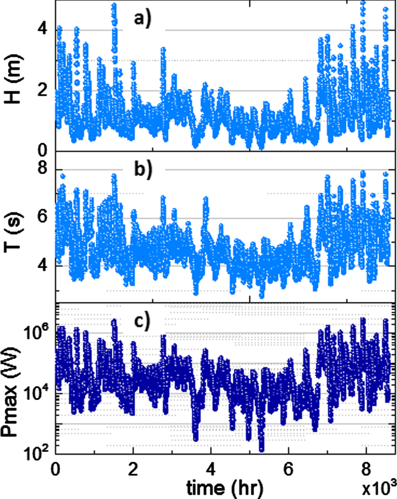
Time series of (a) Hm(t) and (b) T(t) recorded hourly at the Campeche buoy in 2014 (8760 data points). (c) The corresponding wave’s power estimation using the Salter-Falnes model.
Figure 1(c) clearly illustrates the problem at hand: by using the raw series of (Hm, T) pairs from the database, the wave power estimations end up spanning over several orders of magnitude, thus making it difficult to use these results for design purposes. In general terms, like we discuss in the Introduction for other scenarios, this is because the fluctuations in the time series of each variable, Hm(t) and T(t), are amplified through the calculations due to the nonlinear dependence of the wave power on these parameters, Pmax ∝ Hm2T3. This is further verified by calculating some representative values of the wave power data shown in Fig. 1(c). We calculated the mean to be 83.58 kW (±172.10 kW); the median (2nd quartile, Q2, of the full series), 29.47 kW; and the rms power, 191.32 kW.
One can attempt to reduce the effects of this large variability by several means. For instance, in a first-order approach, one could first reduce each time series Hm(t) and T(t) to a single representative value e.g., mean, median, rms value, or largest-probability value, and then estimate Pmax based on a single (Hm, T) pair. Unfortunately, this does not solve the problem. The estimation of Pmax based on the mean values of Hm(t) and T(t) gives 39.63 kW; based on the median, 29.31 kW; based on the rms value, 53.41 kW; and, based on the value of largest probability in each marginal distribution, after fitting to a log-normal distribution, it gives 15.50 kW. As it can be noticed, using the raw data, and reducing the time series to a single value results in estimations with large variability which, in turn, would result in large over/under-estimations of the design considerations.
An improvement over the previous approach is to model the joint probability distribution p(Hm, T) by recognizing that Hm(t) and T(t) are not independent random variables [17, 18]. This is true for the time series Hm(t) and T(t) explored in this work. In fact, the Pearson correlation coefficient between the year-long datasets shown in Fig. 1(a)-(b) is rather high, r = 0.8389, which tells that there exists a strong linear dependence between Hm and T, as verified in Fig. 2(a), where we plotted the entire collection of (Hm, T) pairs recorded over the course of one year. Fig. 2(a) shows basically the same data in Fig. 1(a)-(b) where the time dependence has been removed.
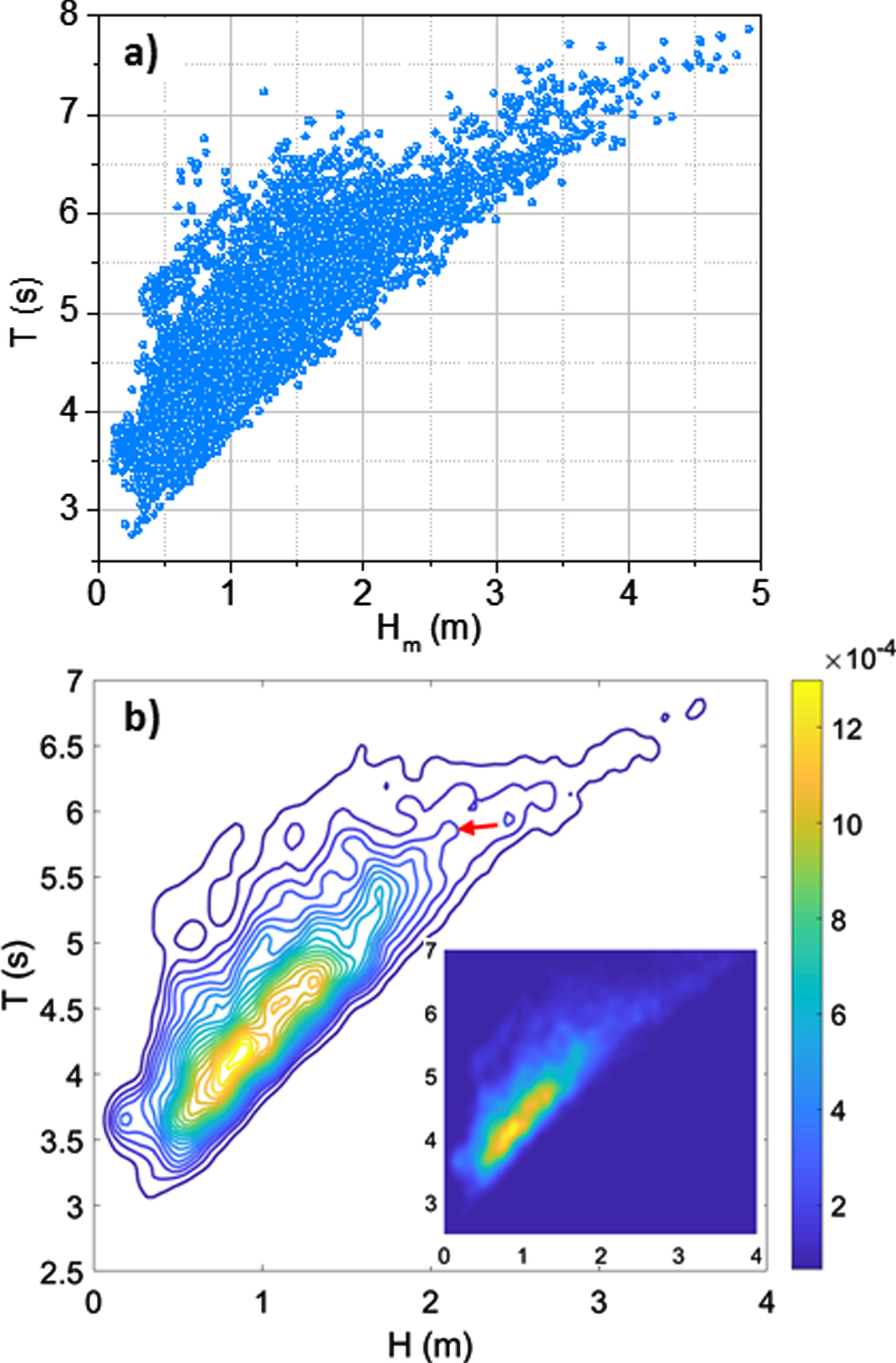
(a) Distribution of the ordered pairs (Hm, T) recorded over the course of one year (raw data) and (b) the corresponding bivariate probability density function p(Hm, T). The red arrow indicates the contour taken to illustrate the proposed approach.
In Fig. 2(b) we show the corresponding probability distribution p(Hm, T) of the data in panel (a) both as a collection of equiprobability contours and as a continuous surface (inset). The values of p(Hm, T) were calculated using an adaptive kernel density estimation by following the work of Botev’s et al. [19]. This is basically a nonparametric probability density estimation that is useful for the case when the joint probability has an arbitrary shape.
In our approach, we essentially propose using p(Hm, T) of the raw data to generate a new series of random (Hm, T) pairs that are contained within an equiprobability contour of p(Hm, T) with a desired probability coverage. As we will show later, this approach is useful to generate a new time scale-independent series that preserves the probability of the measurements to the degree desired, and where the high variability due to the data fluctuations is suppressed. An overview of the proposed methodology is illustrated in Fig. 3. In the following, the steps involved are explained in detail.
Once p(Hm, T) is calculated, then an equiprobability contour is selected based on the desired coverage of p(Hm, T). For instance, the contour indicated in Fig. 2(b) covers around 80% of p(Hm, T). If a higher-valued contour is chosen, a smaller portion of p(Hm, T) will be covered but, in all cases, the region of largest probability is contained regardless of the contour selected. In the limit where the highest-valued contour is selected, only the (Hm, T) pair of largest probability will be accounted; conversely, in the limit when the lowest-valued contour is selected, the entire distribution will be considered.
In the next step, the contour selected is used as a closed boundary in the (Hm, T) plane for the generation of N random (Hm, T) pairs. Because we estimated p(Hm, T) based on the raw measurements, all the contours have irregular shapes that are different from one another (see Fig. 2(b)). To deal with this, we triangulate the region defined by the contour using a Matlab implementation of the standard Delaunay method [20], as shown in Fig. 4(a).
The algorithm for the generation of new (Hm, T) pairs based on the triangulation of the selected contour is explained as follows. For each triangle, we determined its area and associated a probability based on its relative fraction with respect to the total area. Using this area-based probability, we pick triangles randomly and generated a random number inside of it. In this way, the region of the (Hm, T) plane within the equiprobable contour selected is uniformly sampled. In practice, we did this in a fully vectorized manner to generate N samples in a single step. In Fig. 4(b) we show the result of the generation of N = 8760 samples, a new data series of the same length as the original data.
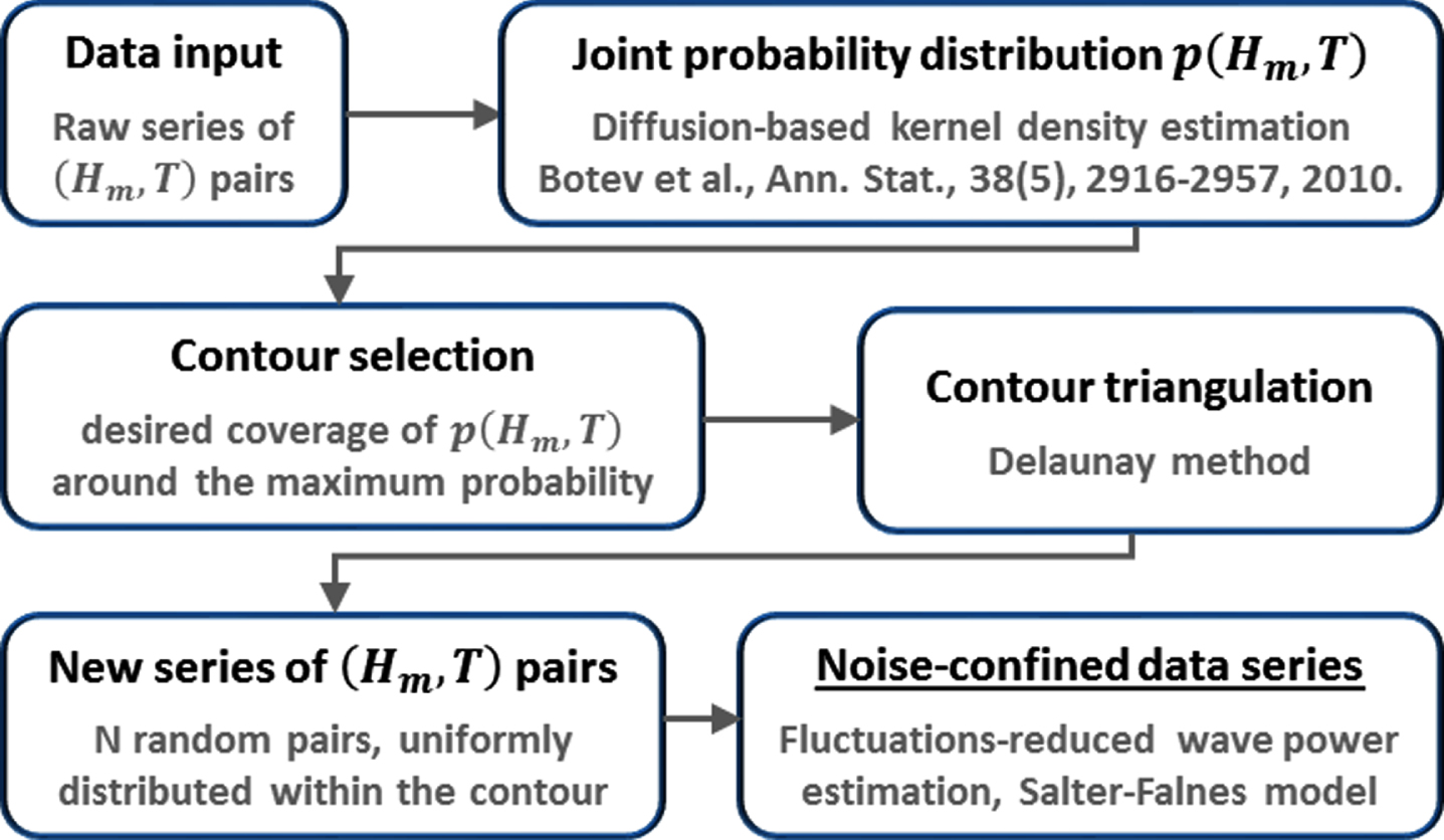
Overview of the methodology proposed for the generation of noise-suppressed data series that preserve the statistics of the original data.

(a) Standard Delaunay triangulation of an equiprobability contour of p(Hm, T) and (b) the corresponding series of (Hm, T) random pairs generated based on the proposed approach.
The results of the methodology proposed are shown in Fig. 5, in the condensed form of a box plot representation. We plotted the statistics of the original measurements (Fig. 1) and those of the randomly generated shown in Fig. 4(b). The red markers indicate the outliers based on the standard criterion of the interquartile range (IQR = Q3-Q1), 1.5IQR<Outliers<3IQR, where Q1 and Q3 are the first and third quartile, respectively.
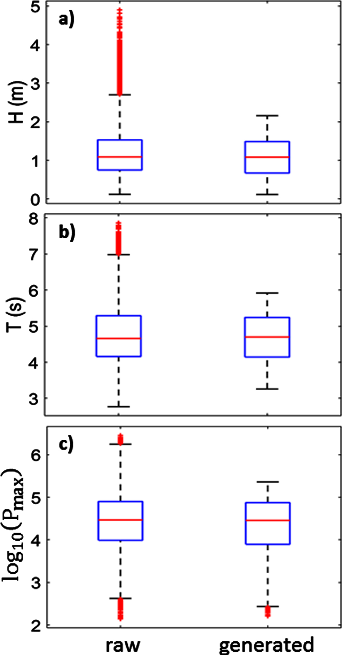
Box plots of the raw measurements and the randomly generated data of (a) Hm, (b) T, and (c) Pmax.
In Table 1, we show a comparison of the calculations obtained using the raw data and the proposed approach. Basically, we calculated Pmax based on the Salter-Falnes formalism described above, when using a single (Hm, T) pair or the entire series, for both the raw data and the generated series. For instance, if one takes the mean of Hm(t) and the mean of T(t), the calculation of Pmax gives 39.63 kW and 29.78 kW for the raw data and the generated series, respectively. If one performs the calculations over the entire series Pmax(t) and analyze its probability distribution, then the mean value of Pmax is 88.11 kW and 48.33 kW for the raw data and the generated series, respectively.
Comparison between the power calculations using the raw data and the data generated using the proposed methodology
As can be seen in Fig. 5 and Table 1, the outcome of our approach is evident: the large-amplitude fluctuations are suppressed while preserving the main features of the original statistics, as indicated by the three quartiles. A direct consequence is that the characteristics of the data series generated, where the noise due to extreme values has been reduced, can now be used for design purposes.
As mentioned before, the independent series Hm(t) and T(t) can be described by log-normal distributions. Because the extreme values are neglected, the tails of the distribution are effectively suppressed. Therefore, our approach can also be thought as an approximation to a quasi-Gaussian distribution. In other words, the generation of new (Hm, T) pairs within the contour selected preserves the bell shape of the original distribution with shorter tails, as illustrated in Fig. 5.
We should also note that the standard Delaunay triangulation deals with the contour as a convex polygon, as shown in Fig. 4(a). For our purposes, this is irrelevant, since only small portion of the points are generated outside the contour, as can be seen in Fig. 4(b). Nevertheless, in order to fully contain the N random samples, accurate two-dimensional triangulation methods are available for arbitrary, non-convex contours (see, for instance, [21]).
Finally, from the analysis presented, we noted that using the raw values for the wave power calculations tends to overestimate the values obtained. Conversely, if a single (Hm, T) pair is used, the calculations are underestimated. Our approach constitutes an intermediate solution. The new series of (Hm, T) pairs is confined to a region of p(Hm, T) where extreme outliers are excluded and, therefore, the fluctuations are suppressed as compared to the raw measurements, while keeping the main statistical features of the original data.
We present a simple methodology based on the use of joint probability distributions that allow suppressing large-amplitude fluctuations of the data, caused by the extreme points, while preserving the essential statistics. To illustrate our approach, we used measurements of sea wave’s significant height (Hm) and period (T). The core of the proposed methodology relies on modeling the joint probability distribution p(Hm, T), and then using an equiprobability contour to generate a new series of random (Hm, T) pairs that are contained within the contour selected. Importantly, the new series of random data is realistic since it was generated from p(Hm, T), which is based on the measurements. Moreover, the new data series is also independent of a time scale. In other words, if p(Hm, T) is assumed to be invariant, one can associated an arbitrary time scale to the randomly generated series. In a way, our methodology can be thought a statistical interpolation and it can make the new series generated useful, for instance, as the input of simulations that require finer time scale in comparison with the sampling time of the measurements. Finally, because large-amplitude fluctuations are suppressed, the randomly generated data can be useful. In the particular example taken in this work (sea wave power), the estimations based on the fluctuations-suppressed data can be useful for the design of sea wave generators.