A machine learning-based weather prediction model and its application on smart irrigation

Abstract

Weather prediction is paramount for many applications and scenarios, among them is agriculture. In order to efficiently irrigate the crops with the exact needed water amount, weather forecasting can be used to optimize the quantity of required irrigation water such that the crops are neither dried up nor over-irrigated. This paper proposes a Machine Learning (ML)-based weather forecasting model, which utilizes the Social Spider Algorithm-Least Square-Support Vector Machine (SSA-LS-SVM) algorithm. The simulation results are used to predict the prime weather and soil parameters such as the atmospheric temperature, pressure, and soil humidity for 24, 48, and 72 hours based on previous 39 days’ hourly data for Amman city. The predicted values showed low relative mean square errors compared with the actual values and the LS-SVM predictor.

Keywords

Weather forecasting prediction smart irrigation artificial intelligence social spider algorithm-least square support vector machine least square support vector machine

1 Introduction

Artificial Intelligence (AI) and Machine Learning (ML) are emerging technologies that have been utilized and used in many several applications and scenarios. Smart agriculture is one of these application that needs such technologies, where it is important to be able to predict the weather conditions to be able to determine the proper irrigation amount for agricultural area. Nowadays, although, with a boost from progressively effective high-performance computers and gigantic loads of information, researchers are starting to apply ML to form more exact and granular forecasts [1]. Thus the innovation is coming together to provide superior climate forecasts for the next coming years, as well as more pinpointed climate forecasts that advertise greater caution for individuals in need of protection from events such as tornadoes and typhoons [2]. An effective variation of prescient innovation might be working within another three to five years. Agriculture currently uses 70% of the withdrawn freshwater [3]. Thus, it is of essential significance that we observe irrigation control, particularly in semi-arid areas with a lack of rainfall. Efficient Irrigation control and management is one important subject of precision agriculture, wherein the best quantity of water is artificially added to a place to fulfill the crop’s needs, and the actual manufacturing of the customers is analyzed [4]. The irrigation has to deliver the crop water requirements at distinctive development levels in a specific region. Irrigation control is used to determine the proper irrigation time, the quantity of irrigation water, and the irrigation frequency, primarily based on tracking evapotranspiration of the crop and soil moisture conditions. Crop evapotranspiration is a measurement of water intake through plants based on the crop’s growth stage and weather conditions [5, 6]. The soil moisture affects the quantity of water irrigation given to the crop, as irrigation control considers the extent of water retaining within the soil. Consequently, precise agriculture could diminish water intake in the irrigation process by taking into consideration the ground water that is available to the crop [4, 6]. The desire for a pleasant irrigation control plan relies upon the records from the tracking field. Using up-to-date technologies, a clever agriculture device collects and organizes data for irrigation control from a variety of sources [6, 7]. Users can offer the capabilities of various forms of crop, soil, and irrigation devices, in addition to the readings of analog tensiometers, which are soil sensors that are used to estimate the moisture level at certain depths and track factors in a field. Furthermore, automatic weather monitoring stations [6, 8] can offer weather records publicly available via the Internet.

Moreover, the sector might also have sensors, control systems, and actuators that could interact with every different gadget on the Internet of Things (IoT) to offer transparent offerings to the agricultural sector and users [6, 9]. Such offerings are associated with irrigation control for tracking (i.e., water quantity, soil moisture level, and air humidity) and prediction (climate and soil conditions). It is worth mentioning that industrial sensors for structures aimed at agriculture and its irrigation process are costly, making it difficult for smaller scale farmers to put this form of the machine into effect on their farms.

However, producers are presently imparting low-value sensors linked to nodes to put into effect low-value structures for irrigation control and agriculture track. Furthermore, because of the wide-spread usage and availability of low-value sensors for tracking agriculture and water. In addition, several new low-value sensors such as a leaf water strain-tracking sensor [10], are being proposed in research. A multi-degree soil moisture sensor produced from copper earrings located alongside a Polyvinyl Chloride (PVC) pipe [11], a water turbidity sensor created using colored and infrared led transceivers [12], or a water salinity tracing sensor created with copper coils [13, 14]. Several works for weather prediction using Least Square Support Vector Machine (LS-SVM) have been proposed in the literature [15, 16]. In [15], the authors presented an irrigation forecasting model based on LS-SVM, which outperformed other techniques such as Back Propagation – Artificial Neural Network (BP-ANN). Furthermore, the authors in [16] provided an improved Least Square Support Vector power load forecasting approach. The difference between the expected and actual values is calculated using the proposed method and the forecast error is utilized to forecast the present prediction error. The proposed load forecasting method accurately estimates the load situation in a given region, compared with a two-stage predicting analytical model of realistic operating maximum load in a specific commercial area. In fact, this paper continues our previous efforts [17] in designing a AI based- remote sensing and weather prediction system that can be used for smart irrigation and farming, where the proposed system utilized Long Range Wide Area Networks (LoRaWAN) [18 –20] and cloud computing [21, 22] technologies for network connectivity, and the Wind Driven Optimization – Least Square Support Vector Machine (WDO-LS-SVM) for weather prediction purposes.

However, according to the conducted literature review, our work is proposing for the first time to utilize the Social Spiral Algorithm jointly with the LS-SVM, shows outstanding performance when compared with the LS-SVM. The rest of the paper is structured as follows. Section II discusses the proposed weather prediction model. Section III presents the research methodology. The simulation outcomes are presented in Section IV. Finally, section V concludes the paper and proposes future work.

2 The proposed prediction model

2.1 Social spider algorithm (SSA)

Spiders can be found anywhere in the world. The spiders, in their nature, have various strategies for foraging, and the most common approach is to find prey by sensing vibration. Spiders have a high sensitivity to the stimulation of vibratory. The vibration on the spider’s webs tells them to catch prey on their webs, whereby if the vibrations are within a particular frequency range, spiders invade the source of the vibration. The actual social spiders can differentiate if the vibrations are produced by prey or by other spiders on the web [23].

In optimization problems, the search space should be formulated as a large spider web. Thus, each spider’s location on the web is a potential solution to the optimization problem. In the meantime, all possible solutions to the optimization problem are in their proper position on this web. However, spiders in SSA have considered SSA agents performing optimization, so you need to identify the spiders’ number at the beginning of the algorithm. Therefore, each spider has a memory that stores the following information; (i) the spider(s) position on the web. (ii) The suitability of the spider’s current location. (iii) The vibrating target $v_{s}^{tar}$ of the preceding iteration. (iv) The number of iterations since the last spider position changed its vibrating target. (v) Movements carried out in the previous iteration. Finally, (vi) the dimension mask used to direct the movement in the preceding iteration. The first two information (spider’s position and vibrating target) describe the spider situation, while the rest information are involved in guiding the spider to a new position.

On the other hand, vibration is a crucial notion in SSA. This feature differentiates SSA from other metaheuristics. In SSA, two possessions are used to define a vibration, particularly the location of the source and the intensity level of the vibration source. The optimization problem’s search space determines the source position, and the vibration intensity level is defined in the interval [0,+∞). Each time the spider transfers to a new location, it generates vibrations at that location. The location of the spider a is defined at time t as P_a (t), or just as P_a. Furthermore, intensity values are drawn after several considerations, including; (i) all conceivable vibrations strength of the optimization problem is positive. (ii) Positions with more suitable values, i.e., lesser values for the minimization problem, have higher vibration intensity than those with poorer fitness values. (iii) As the solution converges towards the global optimum solution, the vibration strength does not increase significantly and causes vibration reduction scheme to fail. In SSA, there are always three stages: initialization, iteration, and finalization. These three steps are performed sequentially. In every run of SSA, it must starts with the initialization phase, after that it iterates search and finally ends the algorithm and returns the obtained solution. In the initialization phase, the algorithm defines the main objective function and its solution domain. Values for parameters utilized in SSA are also set. After the values are set-up, the algorithm produces an initial population of spiders that will be utilized to solve the optimization problem; along with a fixed allocated memory size to them to store their information. The spider’s position is created in the search space with its fitness value estimated and saved. For each spider in the population, the initial target vibration is set to its current location, the intensity of the vibration and all other attributes stored by each spider is set to zero. Therefore, the iteration stage starts, which searches with the created artificial spider. In this step, the algorithm performs several iterations.

With each iteration, all spiders distributed on the web change to a new location and estimate their fitness values. Each iteration can be separated into the succeeding sub-steps, including; (i) fitness assessment, (ii) vibration generation, (iii) mask altering, random navigation/walk, and (iv) constraint management. At the end of the algorithm, it returns the top solution with the best fitness is determined. These three previous steps form the complete SSA algorithm. The algorithm pseudo-code is shown below [23], and we would refer the reader to reference [23] for more information about the SSA algorithm.

3 Methodology

This section specifies the methods and techniques used in achieving the prediction model proposed in this paper. Figure 1 illustrates the approach of the proposed prediction model which do the prediction using a new regression scheme named as the Social Spider -Least Square- Support Vector Machine (SSA-LS-SVM) algorithm as will be illustrated below.

Table 1

Algorithm: SOCIAL SPIDER ALGORITHM

1: Assign initial values to the SSA parameters.

2: Generate the spiders’ pop population and allocate memory resource for them.

3: For every spider, Initialize $v_{s}^{tar}$

4: while ending condition not reached do

5: for each spider s in pop do

6: Calculate the fitness value of s.

7: Create a vibration at s location

8: end for

9: for each spider s in pop do

10: Calculate the vibrations V intensity generated by spiders.

11: Find the strongest vibration $v_{s}^{best}$ from V.

12: i f $v_{s}^{best}$ intensity is >than $v_{s}^{tar}$ then

13: Store $v_{s}^{best}$ as $v_{s}^{tar}$ .

14: end if

15: Updatec_s //wherec_sis the number of iteration since spider s has latter varied its target vibration

16: Generate a random number r from [0, 1).

17: if r > $P_{c}^{c_{s}}$ then // $P_{c}^{c_{s}}$ is a generated random number between (0,1)

18: Adjust the mask dimensionm_s.

19: end if

20: Produce $P_{s}^{fo}$ // $P_{s}^{fo}$ is the new following position of the spider s.

21: Execute a random navigation/walk.

22: Handle any violated constraints.

23: end for

24: end while

25: Product the best determined solution.

Algorithm: SOCIAL SPIDER ALGORITHM
1: Assign initial values to the SSA parameters.
2: Generate the spiders’ pop population and allocate memory resource for them.
3: For every spider, Initialize $v_{s}^{tar}$
4: while ending condition not reached do
5: for each spider s in pop do
6: Calculate the fitness value of s.
7: Create a vibration at s location
8: end for
9: for each spider s in pop do
10: Calculate the vibrations V intensity generated by spiders.
11: Find the strongest vibration $v_{s}^{best}$ from V.
12: i f $v_{s}^{best}$ intensity is >than $v_{s}^{tar}$ then
13: Store $v_{s}^{best}$ as $v_{s}^{tar}$ .
14: end if
15: Updatec_s //wherec_sis the number of iteration since spider s has latter varied its target vibration
16: Generate a random number r from [0, 1).
17: if r > $P_{c}^{c_{s}}$ then // $P_{c}^{c_{s}}$ is a generated random number between (0,1)
18: Adjust the mask dimensionm_s.
19: end if
20: Produce $P_{s}^{fo}$ // $P_{s}^{fo}$ is the new following position of the spider s.
21: Execute a random navigation/walk.
22: Handle any violated constraints.
23: end for
24: end while
25: Product the best determined solution.

Fig. 1

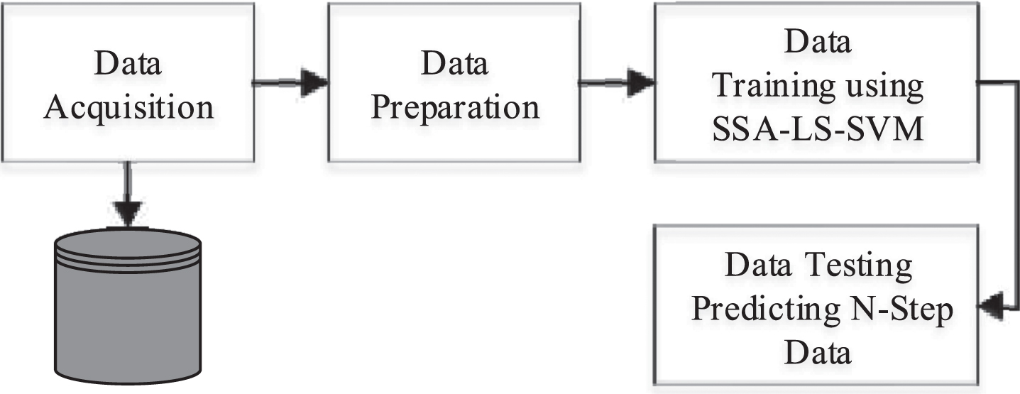
The proposed prediction model approach.

3.1 Data acquisition

Data are acquired by collected weather data related to the capital city of Jordan, which is Amman, from the meteoblue website, where the data is limitedly freely available at this URL: https://www.meteoblue.com/. In this paper, we gathered the amount of 39 days of hourly data between 13 October 2020 and 20 November 2020. The gathered data consists of four main factors representing the weather status, including temperature, humidity, pressure, and soil temperature. Hence, we got 936 samples (39 days * 24 hours) of data for each factor, as mentioned earlier. On another side, in the data preparation step, the data was prepared to be used in the LS-SVM classifier. The data was conceptually cleavage in concept of windowing based on the window length. Thus, in this work, the window sizes of 24, 48, 72 are utilized for 24, 48, 72 hours forecasting, respectively. Therefore, the data is divided into training and testing datasets, where the length of the testing dataset is equal to the window length, and the remaining data is used for training the model.

3.2 Social spider algorithm-least square support vector machine

The SVM classifier was developed to be a quadratic encoding problem involving inequality limitation. That is why an improvement of SVM was recently proposed to solve the issue concerning the equality limitation of the original SVM by solving a system of linear equations, resulting in an enhanced version of SVM named Least Square Support Vector Machine [24]. In addition, LS-SVM is easy to train and takes less computational effort compared with the original SVM.

LS-SVM, includes a Radial Basis kernel Function (RBF), which has two essential parameters include, the regularization parameter γ, as well as, the smoothing parameter σ, which play fundamental roles in identifying the classifier’s performance. The different values of these parameters continuously show the difference in the classifiers. To tune these two values, numerous studies depend on the default values of the classifier or tuning by the grid search method.

On the other hand, other studies have performed an optimization algorithm to set up optimal values of σ and γ for which the classifier shows the highest performance within a specific classification or regression.

In this paper, the SSA algorithm tunes the parameters used in the LS-SVM classifier to find the optimal values. Three parameters of the algorithm have to be set up at the beginning of the algorithm to guide the searching behavior in the algorithm. (i) ra, which represents the vibration reduction rate when propagating over the spider web. (ii) pc, which determines the possibility of the spiders varying their dimension mask during the random navigation/walk step, and (iii) pm, which represents the possibility of each value in a dimension mask equals to one. Moreover, the population size and the bound of search space must also be determined. Hence, the tuning algorithms were implemented in the lower and upper bands ranges of 0.001– 10000, with a population size of 30 and 100 iterations,, respectively and ‘ra’, ‘pc’, and ‘pm’ parameter values are set to 2, 0.7, and 0.3, respectively. The solution space of the tuning problem of LS-SVM parameters is a D-dimensional space, where D is the parameters number (i.e., 2), including σ and γ parameters.

4 Simulation results

The preliminary simulation results of the performed experiments are presented in this section. Thereby, six tests were conducted, mainly comparing two predictive models; one is with grid search-LS-SVM, while the other one is the proposed SSA-LS-SVM. The Normalized Root Mean Square Error (NRMSE) was used as a suitable performance metric in all experiments. The best prediction model is the one that produces low NRMSE. The results from the six experiments include a prediction for 24 hours, 48 hours, and 72 hours for both prediction models.

Figures 2, 3, and 4 show changes in the four weather forecasting prediction parameters at 24 hours, 48 hours, and 72 hours, respectively. In general, the graph shows that the predicted values of the four factors are not close to the actual values. However, the line related to the SSA-LS-SVM is closer to the actual line compared to the line produced by the standard LS-SVM.

Fig. 2

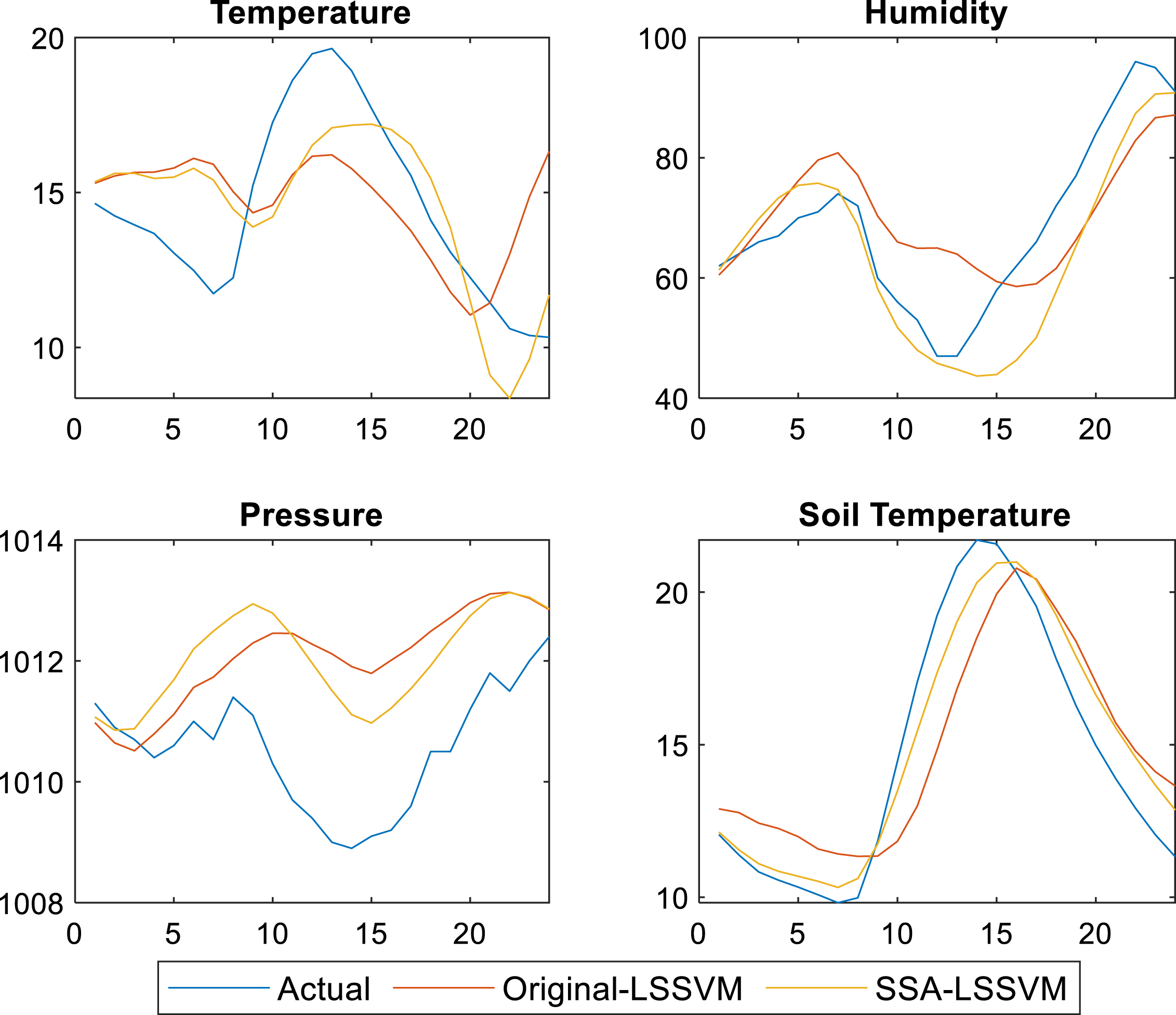
Weather and soil parameters’ prediction for 24 hours using LS-SVM and the proposed SSA-LS-SVM.

Fig. 3

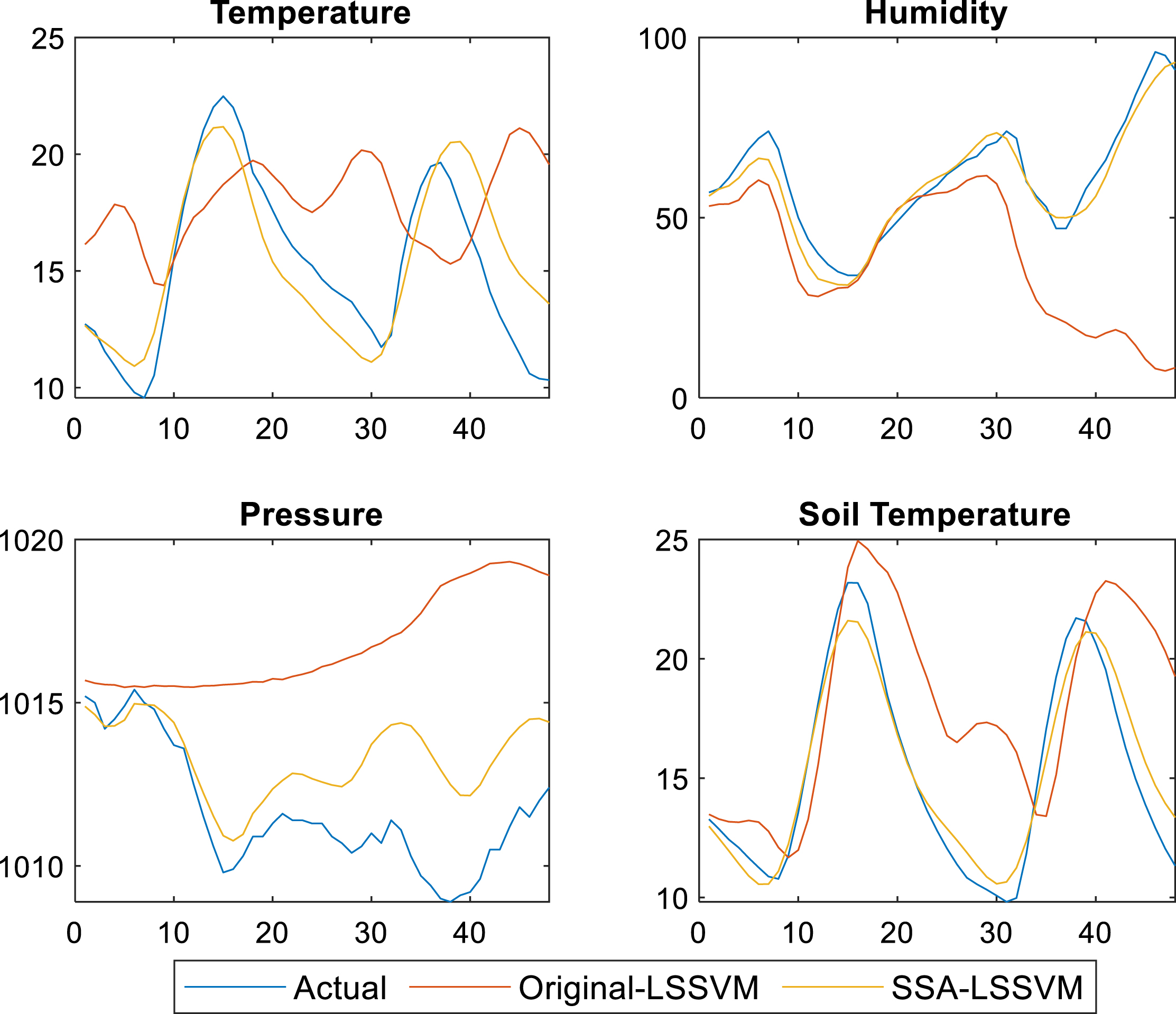
Weather and soil parameters’ prediction for 48 hours using LS-SVM and the proposed SSA-LS-SVM.

Fig. 4

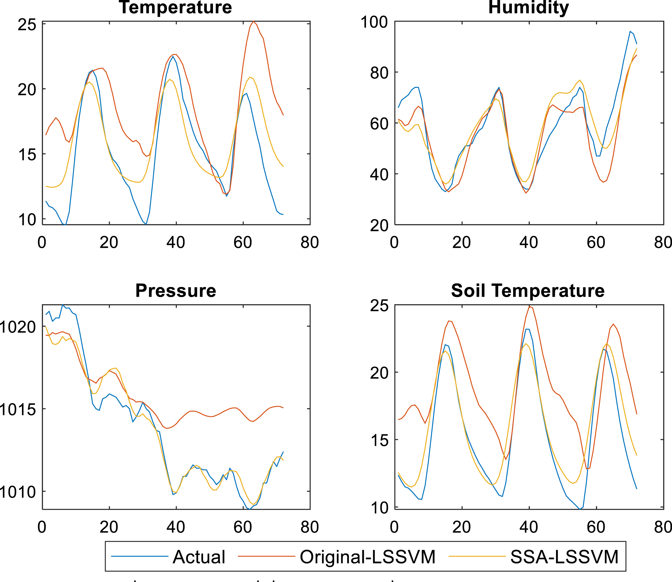
Weather and soil parameters’ prediction for 72 hours using LS-SVM and the proposed SSA-LS-SVM.

Furthermore, Fig. 2 shows that the two lines in pressure lines of both models are not close enough to the actual line compared with the other factors. However, the line of SSA-LS-SVM is still close and mimics the changes of the actual values better than the line of the standard LS-SVM.

On another hand, SSA-LS-SVM outperformance can be clearly shown in the line charts of Fig. 3, whereby its predicted values are highly nearer to the actual values compared with predicted values by the standard LS-SVM. Additionally, there is a noticeable decline in the standard LS-SVMs performance in 48 hours compared to the one using the SSA-LS-SVM. Contrasting the standard LS-SVM, which is tuned with the grid search algorithm, the SSA-LS-SVM is straightforward to the optimum production regardless of the tiny increase of the more extended prediction period.

On another side, Fig. 4 shows line charts of predicting results of 72 hours. Again, the SSA-LS-SVM outperforms the standard LS-SVM, whereby the difference between its line and the actual line is less than the one between the standard LS-SVM and the actual line within several points.

Furthermore, Table 1 depicts the NRMSE prediction results for the standard LS-SVM and SSA-LS-SVM models for the correspondent data of four meteorological (weather) factors. As shown on the results of 24 hours prediction, the highest NRMSE obtained by SSA-LS-SVM, where the values are 0.1660, 0.2195 for relative humidity and temperature, respectively. While the highest NRMSE correspondent to the soil temperature and mean sea level pressure, are 0.0981and 0.4807 respectively. Meanwhile, the highest accuracies obtained by the standard LS-SVM were 0.2978, 0.1917, 0.5307, and 0.1867, respectively.

Table 1

The mean square error for the five predicted weather and soil parameters using the LS-SVM and SSA-LS-SVM

	24 hours		48 hours		72 hours
Algorithm	LS-SVM	SSA-LS-SVM	LS-SVM	SSA-LS-SVM	LS-SVM	SSA-LS-SVM
Temperature	0.2978	0.2195	0.3916	0.1513	0.3544	0.1692
Humidity	0.1917	0.1660	0.5421	0.0666	0.1339	0.1128
Pressure	0.5307	0.4807	0.9093	0.3330	0.2418	0.0724
Soil temperature	0.1867	0.0981	0.3433	0.0776	0.3275	0.1087

On the other side, it can be noticed that the prediction outcomes obtained by SSA-LS-SVM are superior to the prediction outcomes obtained by the standard LS-SVM in all prediction periods. Additionally, the highest NRMSE from experiments are obtained at 48 hours forecasting, where the window size was set to 48 hours. Consequently, it indicates that windowing the data at 48 hours was the best compared with other window sizes include 24 and 72. Meanwhile, the results attained by the standard LS-SVM differ as of one period to another without clear interpretation. The only interpretation is that the standard LS-SVM is tuned by the grid search algorithm, which produces different performances based on the chance of selecting parameters regardless of the direction of optimum values or/and window size of the data.

5 Conclusion

A new prediction scheme namely SSA-LS-SVM is proposed to enhance the accuracy of the standard LS-SVM performance in the prediction process. This model is used to predict whether and soil data such as: the atmosphere temperature, soil humidity, sea level pressure, as well as soil temperature, and compares its performance with the standard LS-SVM prediction model. As a result, the proposed prediction model showed superior performance overall undertaken experiments for different prediction periods. On another side, the SSA could improve the LS-SVM performance by optimizing its parameters, such that the SSA algorithm has excellent performance on searching over a high dimensional space, with high exploration and exploitation capabilities. For future work, this prediction model can be further improved by enhancing the search capability of the SSA. On another side, the factor of window size of the taken data showed a significant effect on the performance of LSSVM; thus, optimizing this factor is recommended.

Footnotes

Acknowledgments

This work is supported by the German Jordanian University seed fund ID SEEIT 02/2018.

References

Fente

D.N.

and Singh

D.K.

, Weather forecasting using artificial neural network, In 2018 second international conference on inventive communication and computational technologies (ICICCT), pp. 1757–1761, IEEE, 2018.

Singh

, Malik

and Arora

, An effective weather forecasting using neural networks, International Journal of Emerging Engineering Research and Technology 2(2) (2014)209–212.

FAO, World Agriculture: Towards 2015/2030—An FAO Perspective; Earthscan Publications Ltd.: London, Uk, 2014.

Haverkort

A.J.

, Ancha Srinivasan (ed), Handbook of precision agriculture, Principles and applications, Euphytica 156(1) (2007)269–270.

Fontenelle

, da Cunha

and Fuckner

, Atlas irrigação: uso da água na agricultura irrigada, Agência Nacional de Águas, Brasília, DF, Brasil, (2017).

GS Campos

, Rocha

A.R.

, Gondim

, Coelho da Silva

T.L.

and Gomes

D.G.

, Smart & green: An internet-of-things framework for smart irrigation, Sensors 20(1) (2020)190.

Voutos

, Mylonas

, Katheniotis

and Sofou

, A survey on intelligent agricultural information handling methodologies, Sustainability 11(12) (2019)3278.

INMET, Brazilian Automatic Weather Station of INMET (Instituto Nacional de Meteorologia). Available online: http://www.inmet.gov.br/portal/index.php?r=esta-coes/estacoesautomaticas (accessed on 29 November 2020).

Borgia

, The Internet of Things vision: Key features, applications and open issues, Computer Communications 54 (2014)1–31.

10.

Daskalakis

S.N.

, Goussetis

, Assimonis

S.D.

, Tentzeris

M.M.

and Georgiadis

, A uW backscatter-morse-leaf sensor for low-power agricultural wireless sensor networks, IEEE Sensors Journal 18(19) (2018)7889–7898.

11.

Guruprasadh

J.P.

, Harshananda

, Keerthana

I.K.

, Krishnan

K.Y.

, Rangarajan

and Sathyadevan

, Intelligent soil quality monitoring system for judicious irrigation, In 2017 International Conference on Advances in Computing, Communications and Informatics (ICACCI), pp. 443–448, IEEE, 2017.

12.

Parra

L.O.R.E.N.A.

, Ortuño

, Sendra

and Lloret

J.A.I.M.E.

, Low-cost conductivity sensor based on two coils, In Proceedings of the First International Conference on Computational Science and Engineering (CSE’13), Valencia, Spain, vol. 68, p. 107112, 2013.

13.

Sendra

, Parra

, Ortuño

, Lloret

and De Valencia

U.P.

, A low cost turbidity sensor development, In Proceedings of the Seventh International Conference on Sensor Technologies and Applications (SENSORCOMM 2013), Barcelona, Spain, pp. 25–31. 2013.

14.

García

, Parra

, Jimenez

J.M.

, Lloret

and Lorenz

, IoT-based smart irrigation systems: An overview on the recent trends on sensors and IoT systems for irrigation in precision agriculture, Sensors 20(4), 1042.

15.

Xie

and Tang

, Forecasting Model of Irrigation Water Requirement Based on Least Squares Support Vector Machine, 2010 International Conference on Intelligent Computation Technology and Automation, Changsha, 2010, pp. 335–338, doi: 10.1109/ICICTA.2010.91.

16.

and Zhu

, LS-SVM Based Two Step Commercial Short-Term Load Prediction, In Proceedings of the 3rd International Conference on Computer Science and Application Engineering (pp. 1–6).

17.

Khalifeh

, Al-Qammaz

, Darabkh

K.A.

, Abualigah

, Khasawneh

A.M.

and Zinonos

, An AI Based Irrigation and Weather Forecasting System utilizing LoRaWAN and Cloud Computing Technologies, In 2021 IEEE Conference of Russian Young Researchers in Electrical and Electronic Engineering (ElConRus), pp. 443–448, IEEE, 2021.

18.

Lavdas

, Zacharioudakis

, Khalifeh

and Zinonos

, The Effect of Temperature and Humidity on Indoor LoRa Propagation Model, in 2021 17th International Conference on Distributed Computing in Sensor Systems (DCOSS), 2021, pp. 374–379.

19.

Shraideh

and Darabkh

K.A.

, Joint Channel and Spreading Factor Selection Algorithm for LoRaWAN Based Networks, in 2020 International Conference on UK-China Emerging Technologies (UCET), 2020, pp. 1–4.

20.

Khalifeh

, Aldahdouh

and Alouneh

, LoRaWAN Energy Optimization with Security Consideration, Int Arab J Inf Technol 18 (2021)476–483.

21.

, Abou-Tair

, Buechsenstein

and Khalifeh

, A fog computing-based framework for privacy preserving IoT environments, Int Arab J Inf Technol 17(3) (2020)306–315.

22.

Tanash

, Khalifeh

and Darabkh

K.A.

, Communication over Cloud Computing: A Security Survey, In 2019 42nd International Convention on Information and Communication Technology, Electronics and Microelectronics (MIPRO), pp. 496–501, IEEE, 2019.

23.

James

J.Q.

and Li

V.O.

, A social spider algorithm for global optimization, Applied Soft Computing 30 (2015)614–627.

24.

Suykens

J.A.

and Vandewalle

, Multiclass least squares support vector machines, In IJCNN’99, International Joint Conference on Neural Networks, Proceedings (Cat. No. 99CH36339), vol. 2, pp. 900–903, IEEE, 1999.