A novel approach for anomaly detection in automatic meter intelligence system using machine learning and pattern recognition

Abstract

Anomaly detection for sensor systems is one of the most researched topics for the Internet of Thing systems. Researchers have been attracted to machine learning classification problems that are considered the most effective techniques. The novel model is proposed by combining anomaly pattern Symbolic Aggregate Approximation (SAX), processing imbalance data and machine learning techniques for sensor anomaly detection. The advantage of anomaly patterns and machine learning leads to the the proposed model to have better performance. The proposed model consists of three phases: finding anomaly pattern features, processing imbalanced data, exploring data by machine learning model. In this paper, the main contributions with respect to previous works can be listed as follows: (i) Successful modeling the new method of SAX for time series data for finding complex and dynamic anomaly patterns. (ii) Archiving applied anomaly pattern feature into machine learning model Random Forest and hyperparameters optimisation of these model. (iii) Fitfully proposed a model combining SAX, imbalance technique, and random forest to anomaly detection. (iv) Achieving applied proposal model in automatic meter intelligence system in Vietnam. The experiential results of the proposed model have described the robustness and better performance for detecting anomalies of power meter sensors.

Keywords

Time series anomaly detection intelligent meter SAX machine learning pattern recognition

1 Introduction

The Internet of Things, (IoT), including electronic sensors and mobile phones, are generators of big data that satisfies variety, velocity, veracity, and variability. The role of IoT are essential of many systems such as a health system, cyber security system, predictive maintenance, industrial automation and fault prevention system. However, researching anomaly detection faces three challenges that are data arriving rapidly and time series data, imbalanced label data, and complex and dynamic anomaly patterns [4, 14]. Thus methods of anomaly detection in sensor systems are attractive not only to academy researchers but also to industrial researchers recently [4 , 16].

Three types of anomalies are considered [6]:

Point anomaly: one point that is the range value of normal point of the time series.

Contextual anomaly: one point is a normal point of the time series but when given some value before and after or the range of value, the anomaly in context occurs.

Collective anomaly: a sub-sequence series extract from the series that does not expect value or match with the normal pattern.

Various techniques of anomaly detection have been developed for application domains [1]. The authors in [19] compare detection techniques (statistical learning, rule-based and machine learning algorithm). Its result for wireless sensor network (WSN) data sets improves performance of machine learning algorithm but with complexity computational. I. Gethzi Ahila Poornima et al. [15] use Online Locally Weighted Projection Regression (OLWPR) and get a good result with low complexity. Another approach is using autoregressive data-driven model and classify anomaly points that deviates significantly from prediction interval [9]. LSTM [13] reconstructs the time series of normal behavior and detect anomalies from reconstruction error. The survey of anomaly detection in sensor researches is described in Table 1.

Table 1
Anomaly detection in sensor researches

Objective Methodology Case Studies Year Pub

Compare performance and and complexity computation of detection techniques Statistical learning, rule based and machine learning algorithm Wireless Sensor Network dataset 2011 [19]

Find an online prediction based anomaly detection with reduced false alarm rates and very limited memory consumption. Online Locally Weighted Projection Regression Wireless Sensor Network dataset 2020 [15]

Develops a real-time anomaly detection method for environmental datastreams that can be used to identify data that deviate from historical patterns Autogressive model and confidence interval Wind-speed sensor data stream 2009 [9]

Develops a LSTM base Encoder-Decoder method for anomaly in time series Long-short term memory space shuttle valve,Power demand and ECG dataset 2016 [13]

Objective	Methodology	Case Studies	Year	Pub
Compare performance and and complexity computation of detection techniques	Statistical learning, rule based and machine learning algorithm	Wireless Sensor Network dataset	2011	[19]
Find an online prediction based anomaly detection with reduced false alarm rates and very limited memory consumption.	Online Locally Weighted Projection Regression	Wireless Sensor Network dataset	2020	[15]
Develops a real-time anomaly detection method for environmental datastreams that can be used to identify data that deviate from historical patterns	Autogressive model and confidence interval	Wind-speed sensor data stream	2009	[9]
Develops a LSTM base Encoder-Decoder method for anomaly in time series	Long-short term memory	space shuttle valve,Power demand and ECG dataset	2016	[13]

From previous studies, it can be shown that there are two main methods for the machine learning approach in time series anomaly detection problems. That is, classification techniques and regression techniques depend on the data set’s property. The classification techniques are mainly used with good anomaly labeled data sets while regression techniques are used when the set of labeled anomalies are not sufficient and diverse that is described in Table 2. In our study, since our data set are well labeled, we use classification techniques as the main method to tackle the time series anomaly detection problem.

Table 2

Machine Learning in Time series anomaly detection researches

Objective	Methodology	Case Studies	Year	Pub
Applying classification techniques for anomaly detection to improve safety and maintenance activities	Random Forest Algorithm, Decision Jungle Algorithm	Data set from a pharmaceutical company	2020	[2]
Investigating prediction-based and pattern recognition-based methods and apply to indoor climate anomaly detection	Recurrent Neural Network, LSTM-encoder-decoder	Indoor climate data of vertical plant wall systems	2020	[11]
Comparing performances of several machine learning models in predicting anomalies on the IoT systems	Logistic Regression, Support Vector Machine, Decision Tree, Random Forest, Artificial Neural Networks.	DS2OS traffic traces data set from Kaggle	2019	[8]

Symbolic aggregate approximation (SAX) is a method that transforms a time series into discrete symbolic sequences [3, 20]. It is widely used in many subjects such as pattern recognition, anomaly detection. The authors in [5] use HOT-SAX algorithm to detect anomalies in water management. TSAX [21], SAX_CP [20], TrSAX [17] are newly SAX techniques and improve performance [18] in classification. Table 3 shows the survey SAX in time series.

Table 3

SAX in time series researches

Objective	Methodology	Case Studies	Year	Pub
Propose a trend symbolized method (TSAX) to detect theanomaly heart signals	TSAX	ECG (electrocardiography) dataset	2019	[21]
Compare performance of ARIMA and HOT-SAX method for anomaly detection	HOT-SAX	Water management system	2019	[5]
Propose trend base SAX reduction techniques	SAX-CP	UCR time series dataset	2019	[20]

One of the challenging tasks of anomaly detection is imbalanced data. It makes classification less effective in a minor class, which is the anomaly class [12]. There are various techniques to solve the problem: oversampling the major class, under-sampling the minor class, or combine over and under-sampling methods.

In this paper, a combination of time series pattern analysis and machine learning techniques is investigated into the problem of sensor anomaly detection. Selection techniques of anomaly pattern Symbolic Aggregate Approximation (SAX), data balance data and machine learning modeling are integrated to detect anomaly sensors.

The paper is organized into four sections: Section 2 shows the methodology of anomaly detection, SAX, imbalance and the proposed model are presented. The experiments and results of the smart meter sensor are shown in Section 3. Lastly, the conclusion and discussions are provided in Section 4. In addition, some notations are summarised in Table 4.

Table 4

Table of nomenclature

Name	Description
AR	Autoregressive
ARMA	Autoregressive Moving Average
ARIMA	Autoregressive Integrated Moving Average
DT	Decision Tree
IoT	Internet of Things
PAA	Piecewise Aggregate Approximation
RF	Random Forest
SARIMA	Seasonal Autoregressive Integrated Moving Average
SAX	Symbolic aggregate approximation

2 Methodology

2.1 Anomaly detection formula problem

In this paper, an energy meter is a sensor that measures the automatic electricity load of a consumer by time. This sensor is binary classified into anomaly and normal. If the sensor has an anomaly status, it will inspect and check.

Sensor data set has an input with N features: x = {x¹, x²,…,x^N}. The aim of the classification problem is to find each sensor that belongs to either of two classes {anomaly, normal} as correctly as possible.

Consider the data of a sensor $S = {(x_{i}, y_{i})}_{i = 1}^{n}$ where $x_{i} \in ℝ^{N}$ and y_i ∈ {anomaly, normal} sensor. The objective of the problem is to find the function f (.) as follows y = f (x) .

2.2 Overview anomaly detection system

The research procedure of time series anomaly detection system contains four phases that are described in Fig. 1.

Fig. 1

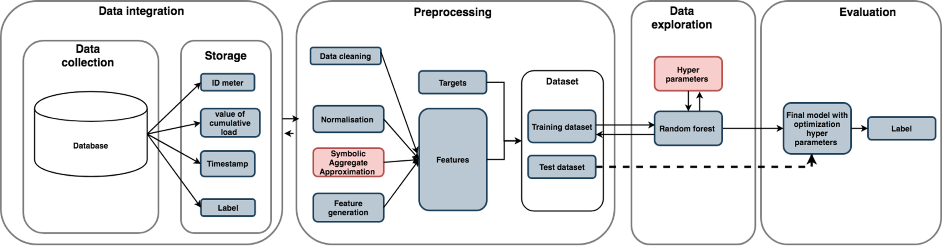
Four phases for anomaly detection sensor system.

Phase 1: Integrating Data: Gathering data from various sources and combining it into one data set.

Phase 2: Pre-processing Data: Raw data collected from the previous step can be in various formats and may be inconsistent. This step involves data cleaning, data normalization and features generation is conducted to overcome this problem.

Phase 3: Modeling: Processed data set will be split into two sets: the training set and the test set. The training set will be used to train a classifier.

Phase 4: Evaluation: This step helps to select the best model corresponding to criteria and evaluate the performance of the selected model in the future. If the model’s performance is poor, go back to the data pre-processing step to clean data and generate more predictive features or the modeling step to tuning the model’s hyper-parameters.

2.3 Symbolic aggregate approximation (SAX)

SAX algorithm proposed by Lin el al.[3] is a classical symbolic approach in data mining applications of time series data. In this paper, the novel SAX is proposed for pattern recognition of the time series data of a sensor.

Time series of the energy meter is generated by consumer activity. The behavior of humans has seasonal daily, weekly, monthly, and yearly patterns. The behavior patterns are created from historical data that difficult to process for the usual time series statistical analysis such as AR, ARIMA, SARIMA, SARIMAX, and spectral models.

A new method to find a normal pattern of seasonal with w time step are described below:

Step 1: Consider a time series of length n: X = {x_{t
₁}, x_{t
₂}, …, x_{t
_n}}, in the observed time period T = [t₀, t_n].

Step 2: Select a fixed size of window w and divide time series into $M = ⌈ \frac{n}{w} ⌉$ equal parts:

$P (1) = {x_{t_{0}}, \dots, x_{t_{w}}}$

$P (2) = {x_{t_{w + 1}}, \dots, x_{t_{2 w}}}$ ⋮

$P (M) = {x_{t_{(M - 1) w + 1}}, \dots, x_{t_{Mw}}}$

Thus the original data now is represented by M window

X = {P (1), P (2), \dots, P (M)} .

The normal symbolic pattern for data in window is defined in the next step. Step 3: Let set

P^{i} = {{x_{t}}_{j}}_{j = 1}^{w}

, i = 1, …, M is the list of data in period i. Then, separating the list values of time series data into l quantiles. Consider

Q^{i} = {q_{k} i}_{k = 1}^{l}

, where

q_{k}^{i} = quantile (P^{i}, \frac{k . 100}{l} %)

is the list of quantile values of set

P^{i}

. In the period i, l split thresholds are defined

q_{1}^{i}, q_{2}^{i}, \dots, q_{l}^{i}

that depends on the Set

P^{i}

and parameter l. The symbolic

A = {a_{1}, \dots, a_{l}}

are used to decode data in the next step.

Step 4: $P^{i} = {{x_{t}}_{j}}_{j = 1}^{w}$ , the time series period i that x_t_j is decoded value by symbol $a_{k} \in A$ if ${x_{t}}_{j} \in [q_{k}^{i}, q_{k + 1}^{i}]$ which k ∈ {1, …, l}. Then, the parts $P^{i}$ can be represented as $Symbol (i) = (a_{1}^{i}, \dots, a_{w}^{i})$ , i = 1, … M and $a_{j}^{i} \in A, \forall j = \bar{1, w}$ as follows:

$Symbol (1) = {a_{1}^{1}, \dots, a_{w}^{1}}$

$Symbol (2) = {a_{1}^{2}, \dots, a_{w}^{2}}$ ⋮

$Symbol (M) = {a_{1}^{M}, \dots, a_{w}^{M}}$

Each symbolic vector has w positions that run from 1 to w. The set of all symbolic at position j of M symbolic vector has form

B_{j} = {a_{j}^{1}, \dots, a_{j}^{M}}

a_{j}^{mode} = mode (B_{j})

the most frequency symbol at the position j. Thus the mode vector is the most frequent symbolic occur that called a normal pattern. Given

{Symbol}_{normal}

is the normal behavior of time series defined by the formula:

{Symbol}_{normal} = {a_{1}^{mode}, \dots, a_{w}^{mode}} .

(1)

The meaning ${Symbol}_{normal}$ is the pattern that represented most frequent behavior of sensor in the window w that learns from the number of windows time series data and label.

Step 5: After ${Symbol}_{normal}$ pattern is found, the analytic the label to see the features different between two classes normal and anomaly sensors. Thus, the distance SAX between a new time series with a normal behavior can be calculated using the following formula: $d_{SAX} = d ({Symbol}_{normal}, {Symbol}_{new}) = symdist ({Symbol}_{normal}, {Symbol}_{new})$

Where mode(.) the statistical operator returns the symbol has the highest frequency of a given set; symdict (.) is Jaccard distance is defined for two symbolic vectors A and B:

$symdict (A, B) = \frac{| A \cap B |}{| A | + | B | - | A \cap B |}$ (2)

Figure 2 shows an example of using SAX to encode time series. The sub sequences of raw time series data in window w are encoded into a symbolic vector using SAX. Figure 3 shows the symbolic anomaly vector using SAX. The anomaly vector is very different from the normal behavior of sensors.

Fig. 2

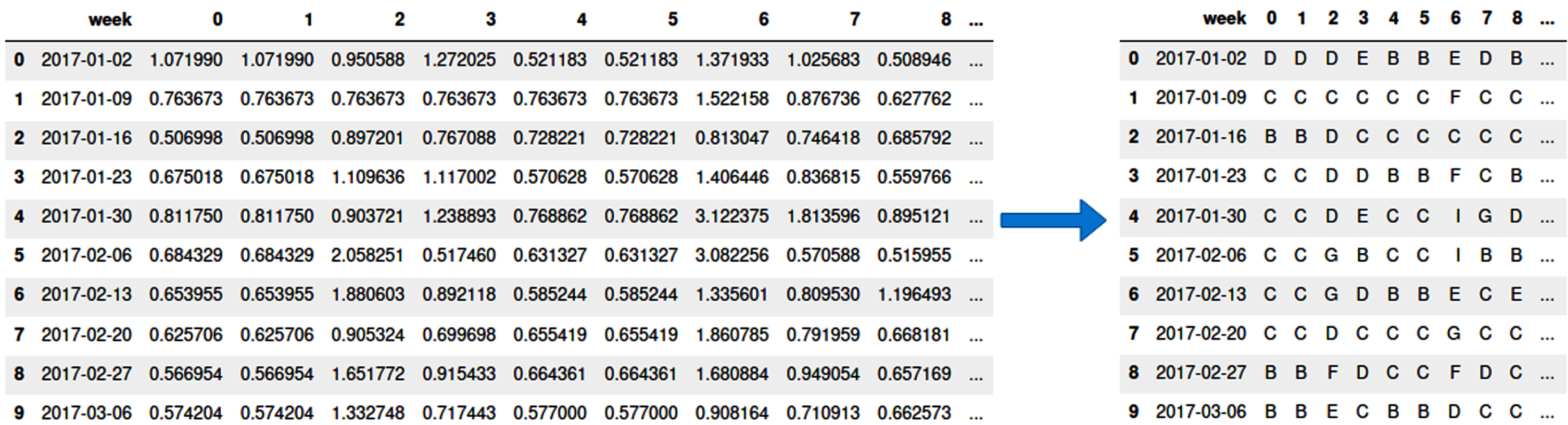
SAX encodes sub sequence time series in window w into symbolic vector.

Fig. 3

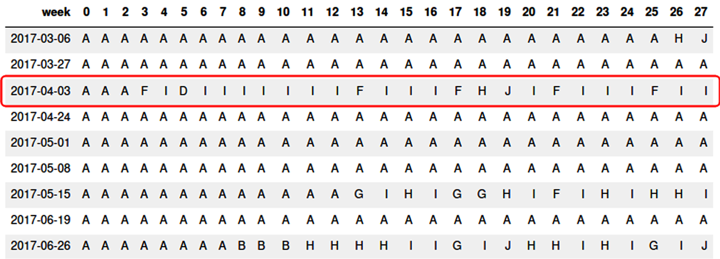
Extract symbolic anomaly vector using SAX

It is using this distance for analyzing the new features of two normal and anomaly classes. The advantage of SAX is tolerated the noise of time series data a and its variance is small, but it can not detect abnormal sub-sequence of w time step.

2.4 Random forest

The random forest model is an effective ensemble learning method, mostly used for classification problems due to their high performance. The random forest model operates by constructing many decision trees (weak-learners) and train them on sub-samples of the data set individually. Finally, the random forest model make predictions by averaging all weak-learners predictions to overcome the over-fitting problems of the weak-learners and ensure consistency [2].

The random forest model applies the bagging technique to train individual tree learners. Given a training set Sensor has an input with N features: x = {x¹, x²,…,x^N} and $X = (x_{1}, \dots, x_{d})^{T} \in ℝ^{N \times d}$ and corresponding labels $y \in ℝ^{N}$ , in each step, bagging sampling with replacement in both instances, and features aspect of the training set then trains individual tree learners with these data set:

For tree = 1, . . . , N:

Sampling M < d instances examples and k < N features from training data set $X$ , y with N features and d instances to create sample training set $X_{tree} \in ℝ^{M \times k}, y_{tree} \in ℝ^{M}$ .

Train a classification tree f_tree (.) on $X_{tree}, y_{tree}$

After training, the random forest model makes a prediction for an unknown label instance x by taking the majority vote or the mean of the predictions from all the individual trained tree learners on x:

\hat{y} = \frac{1}{tree} \sum_{tree = 1}^{N} f_{tree} (x)

This bagging process of the random forest model pay a role in de-correlating the single tree learners that help to the decrements in the variance of individual model prediction without increasing the bias.

2.5 Proposed model

The data set of sensors include cumulative time series, which represent power consumption per unit time. In this section, the workflow of the proposed model is described below. It consists of three main stages:

Pre-processing: Transform original time series data to consumption time series. Then, normalize them based on the time period per day.

Feature engineering: Create feature from processed data. After that, add statistic features an $\bar{d}$ generate a new feature using SAX algorithm. With collected features data set for each object, it is split into train set and test set.

Modeling and evaluate: Apply imbalance processing techniques for the train set. Then it’s trained using the random forest model with selected hyperparameters. We evaluate and choose a trained model with optimized hyperparameters.

We visualize output and testing the final model by using evaluation metrics. The overview model of this approach is shown in algorithm Figure 4, respectively.

Fig. 4

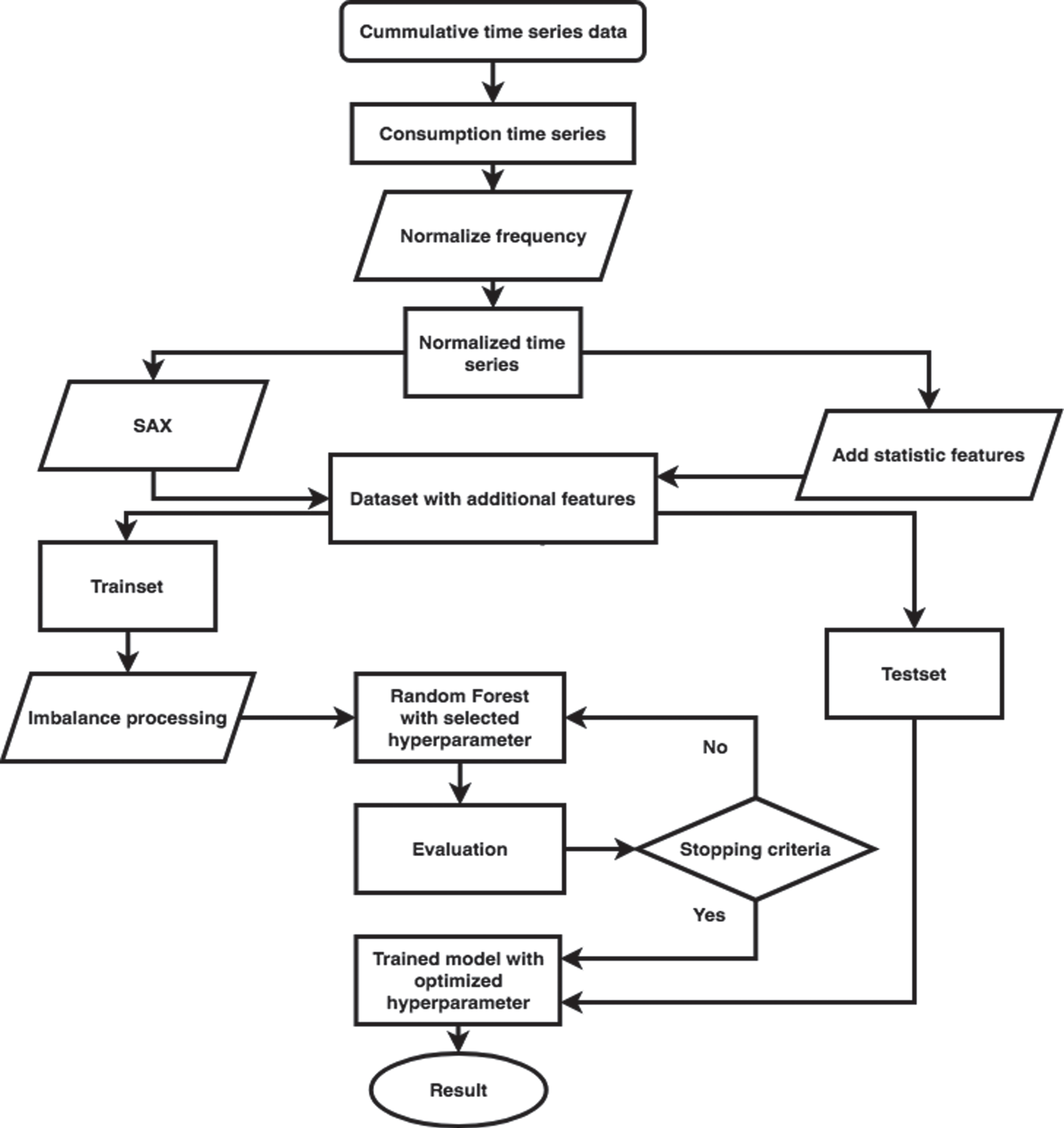
Proposed model anomaly detection using machine learning and pattern recognition.

Algorithm 1

Pre-processing

Require: Cumulative time series data TS

Ensure: Features set F

1: Transform TS to consumption time series TS′

2: Normalize TS′ to normalize time series TS₀

3: F₀ ⟵ gen (TS₀)

4: F_SAX ⟵ SAX (F₀)

5: F_stat ⟵ stat (F₀)

6: F ⟵ F₀ ∪ F_SAX ∪ F_stat

7: return F

Algorithm 2

The proposed model

Require: Cumulative time series data TS

Ensure: Evaluation metrics E

1: F ⟵ Pre - processing (TS)

2: Split F to train set F_train and test set F_test

3: F_train ⟵ SMOTE (F_train)

4: while stopping criteria do

5: RF ⟵ fit RF model(F_train, n - estimators, max - depth)

6: end while

7: E ⟵ Evaluation (RF (F_test))

8: return E

3 Experiments and results

3.1 Data set description

The data set contains the time series data of the cumulative energy of 1067 sensors from 1/1/2017 to 31/3/2018 in a province of Vietnam. The data include about 2.5 million rows, and 3 attributes are described in Table 5.

Table 5
The description of the data set

Attribute Description Data type

Meter ID The identification of the sensors String

Timestamp The datetime to record data Datetime

Import_KWH The value of cumulative data at timestamp Float

Attribute	Description	Data type
Meter ID	The identification of the sensors	String
Timestamp	The datetime to record data	Datetime
Import_KWH	The value of cumulative data at timestamp	Float

3.2 Evaluation metrics

- -Four measures used in our experiments to evaluate five methods: classification accuracy, Precision, Recall and F₁ score. These criteria are calculated by the following formula:

$Accuracy = \frac{TP + TN}{TP + FP + TN + FN};$ (3)

$Precision = \frac{TP}{TP + FP};$ (4)

$Recall = \frac{TP}{TP + FN};$ (5)

$F_{1} = 2 \frac{Precision \times Recall}{Precision + Recall}$ (6) where:

TP and TN are the proportion of correct classification that positive and negative class data points;

FP and FN are the proportion of incorrect classification that positive and negative class data, respectively.

3.3 Results

We use three scenarios for the experiment, there are:

Scenario 1: Decision Tree with different parameters are applied for data set with 28 based-features.

Scenario 2: The random forest model with different parameters are applied for data set with 28 based-features.

Scenario 3: Use proposed model with different parameters for data set with additional features (28 based-features + feature from SAX algorithm and statistic features).

We use SAX algorithm to calculate the normal behavior of electricity consumption by the week for each meter. Figure 5 shows electricity consumption by week of normal and fraud meters. The big and red lines in each figure represent normal behavior. The figures show clearly that the normal behavior of normal meters is periodic and stable. By contrast, the normal behavior of fraud meters is unstable.

Fig. 5

(a) (b) Graphs of electricity consumption by the week of normal meters. (c) (d) Graphs of electricity consumption by the week of fraud meters

The hyperparameters we fine-tune in the experiment for the proposed model and the random forest model include the number of trees in the forest and the maximum depth of the tree. For the decision tree model, we tune the maximum depth of the tree. The number of trees in the forest we choose are 200, 400, 600, 800, 1000, 1200, 1400, 1600, 1800, 2000, and the maximum tree’s depth are 10, 20, 30, 40, 50, 60, 70, 80, 90, 100. The result of three models with the different sets of hyper-parameters which choosing at random is shown in Table 6.

Table 6

Results of scenario 1, scenario 2, scenario 3

Model	n-estimators	max-depth	Accuracy (%)	Precision (%)	Recall (%)	F1-score (%)
Scenario 1		10	71.46	4.32	62.12	8.09
Decision Tree		20	82.53	5.41	46.36	9.69
		30	87.68	6.48	37.87	11.06
		40	88.59	6.82	36.67	11.50
		50	88.84	6.68	34.84	11.21
		60	88.54	6.69	36.06	11.29
		70	88.54	6.69	36.06	11.29
Scenario 2	200	50	96.80	27.67	36.06	31.31
Random Forest	200	60	96.84	28.23	36.36	31.78
	400	70	96.82	27.40	34.54	30.56
	1000	80	96.88	28.29	35.15	31.35
	1200	60	96.89	28.53	35.45	31.62
Scenario 3	200	50	97.68	44.67	37.68	40.88
Proposed model	200	60	97.65	43.83	37.10	40.18
	400	70	97.66	44.05	36.52	39.93
	1000	80	97.66	43.85	36.23	39.68
	1200	60	97.65	43.71	36.23	39.61

Figure 6 shows the results of the models corresponding to 3 methods. It can make clear be seen from Fig. 6 that, for the decision tree model, the average value of F1-score is approximately 10.85% and the average value of precision is about 6.35%. Similarly, for the random forest model, the average value of F1-score and precision are 28,49% and 24.57%, respectively. For the proposed model, the average F1-score and average precision are 39.32% and 43.38%, respectively. Compared to the decision tree and the random forest model, the proposed model gives us many superior results.

Fig. 6

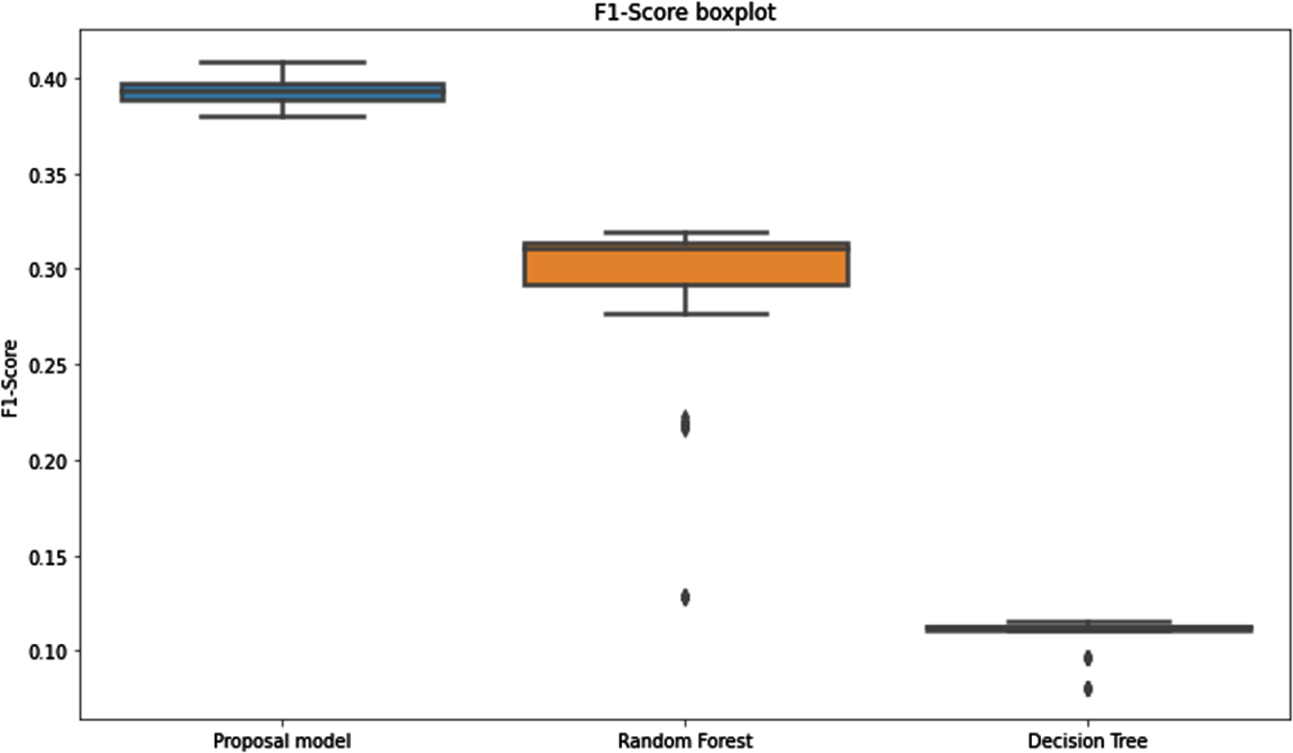
Evaluation metric F1-score of the three methods.

Three precision of three methods is described in Fig. 8. Once more time, the proposed model, the average precision from 39.9% much better than two other method decision tree with average precision 11% and 30.5%. Thus, comparing the average precision of three methods decision tree and random forest model, the proposed model gives high performance.

Fig. 7

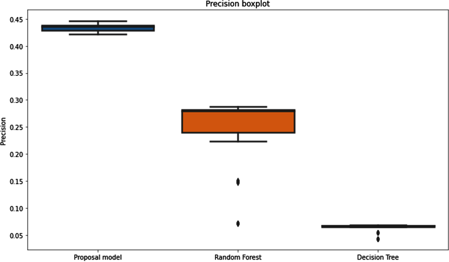
Evaluation metric precision score of the three methods.

Fig. 8

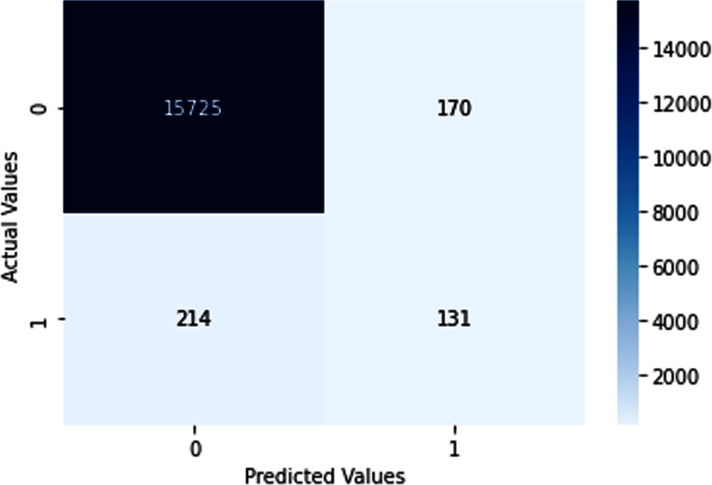
Confusion matrix of proposed model with the best F _ 1 score and precision.

4 Conclusions and discussions

A new proposal model integrates SAX and imbalance for prepare processing, random forest for anomaly detection sensor systems are addressed in our research. Concretely, the contributions of our paper are as follows:

Successful finding complicated and dynamic anomaly patterns using SAX for time series data..

Archiving applied anomaly pattern for machine learning model.

Fitfully proposed a model combining SAX, imbalance technique and random forest to anomaly detection.

Achieving applied proposal model in automatic meter intelligence system in Vietnam.

According to the experimental result, our proposed model has better performance than using well-known machine learning models. The cause of better results are chosen complex and dynamic anomaly patterns in meter intelligence system.

In future work, more sensor anomaly detection applications are researched base on the proposed model. The advanced SAX to find a new pattern will be investigated. The anomaly detection of subsequent of normal symbolic patterns is necessary to study.

Footnotes

Acknowledgment

We want to thank CMC Institute of Science and Technology for supporting this paper.

References

Chandola

, Banerjee

and Kumar

, Anomaly detection: A survey, ACM Comput Surv 41(3), July (2009).

Di Gravio Elena Quatrini

, Costantino

and Patriarca

, Machine learning for anomaly detection and process phase classification to improve safety and maintenance activities, Journal of Manufacturing Systems: SME 56 (2020), 117–132.

Erhan

, Ndubuaku

, Di Mauro

, Song

, Chen

, Fortino

, Bagdasar

and Liotta

, Experiencing sax: a novel symbolic representation of time series, Data Mining and Knowledge Discovery 15 (2007), 107–144.

Erhan

, Ndubuaku

, Di Mauro

, Song

, Chen

, Fortino

, Bagdasar

and Liotta

, Smart anomaly detection in sensor systems: A multi-perspective review, Information Fusion 67 (2021), 64–79.

Gonzalez-Vidal

, Cuenca-Jara

and Skarmeta

A.F.

, Iot for water management: Towards intelligent anomaly detection, In 2019 IEEE 5th World Forum on Internet of Things (WF-IoT), pages 858–863, 2019.

Guigou

, Collet

and Parrend

, Scheda: Lightweight euclidean-like heuristics for anomaly detection in periodic time series, Applied Soft Computing 82 (2019), 105594.

Dahbi

, El Hannani

, Aqqal

and Haidine

, Power audit: an estimation model-based tool as a support for monitoring power consumption in a distributed network infrastructure, International Journal of Advanced Intelligence Paradigms (IJAIP), 13, 2019.

Hasan

, Md. Islam

, Md Ishrak Zarif

and Hashem

M.M.A.

, Attack and anomaly detection in iot sensors in iot sites using machine learning approaches, Internet of Things 7 (2019), 100059.

Hill

D.J.

and Minsker

B.S.

, Anomaly detection in streaming environmental sensor data: A data-driven modeling approach, Environmental Modelling Software 25(9) (1022), 1014–1022. Thematic issue on Sensors and the Environment –Modelling ICT challenges.

10.

Liang

, Song

, Wang

, Guo

, Li

and Liang

, Robust unsupervised anomaly detection via multi-time scale dcgans with forgetting mechanism for industrial multivariate time series, Neurocomputing, 2020.

11.

Liu

, Pang

, Karlsson

and Gong

, Anomaly detection based on machine learning in iot-based vertical plant wall for indoor climate control, Building and Environment 183 (2020), 107212.

12.

Longadge

and Dongre

, Class imbalance problem in data mining review, ArXiv, abs/1305.1707, 2013.

13.

Malhotra

, Ramakrishnan

, Anand

, Vig

, Agarwal

and Shroff

, Lstm-based encoder-decoder for multisensor anomaly detection, ArXiv, abs/1607.00148, 2016.

14.

Malave

and Nimkar

A.V.

, A survey on effects of class imbalance in data pre-processing stage of classification problem, International Journal of Computational Systems Engineering 6 (2020), 65–75.

15.

Gethzi Ahila Poornima

and Paramasivan

, Anomaly detection in wireless sensor network using machine learning algorithm, Computer Communications 151 (2020), 331–337.

16.

Qin

, Yan

and Ji

, Application of controller area network (can) bus anomaly detection based on time series prediction, Vehicular Communications, page 100291, 2020.

17.

Ruan

, Hu

, Xiao

and Zhang

, Trsax-an improved time series symbolic representation for classification, ISA Transactions 100 (2020), 387–395.

18.

Sun

, Li

, Liu

, Sun

and Chow

, An improvement of symbolic aggregate approximation distance measure for time series, Neurocomputing 138 (2014), 189–198.

19.

Xie

, Han

, Tian

and Parvin

, Anomaly detection in wireless sensor networks: A survey, Journal of Network and Computer Applications 34(4) (1325), 1302–1325. Advanced Topics in Cloud Computing..

20.

Yahyaoui

and Al-Daihani

, A novel trend based sax reduction technique for time series, Expert Systems with Applications 130 (2019), 113–123.

21.

Zhang

, Chen

, Yin

and Wang

, Anomaly detection in ecg based on trend symbolic aggregate approximation, Mathematical Biosciences and Engineering: MBE 164 (2019), 2154–2167.

A novel approach for anomaly detection in automatic meter intelligence system using machine learning and pattern recognition

Abstract

Keywords

1 Introduction

2.1 Anomaly detection formula problem

2.2 Overview anomaly detection system

2.5 Proposed model

3.1 Data set description

Table 5 The description of the data set Attribute Description Data type Meter ID The identification of the sensors String Timestamp The datetime to record data Datetime Import_KWH The value of cumulative data at timestamp Float

Footnotes

Acknowledgment

References

Table 5
The description of the data set

Attribute Description Data type

Meter ID The identification of the sensors String

Timestamp The datetime to record data Datetime

Import_KWH The value of cumulative data at timestamp Float