Optimized TOPSIS technique for trajectory selection of self-driving vehicles on highways

Abstract

The selection of an appropriate trajectory for self-driving vehicles involves the analysis of several criteria that describe the generated trajectories. This problem evolves into an optimization problem when it is desired to increase or decrease the values for a specific criterion. The contribution of this thesis is to explore the use and optimization of another technique for decision-making, such as TOPSIS, with a sufficiently robust method that allows the inclusion of multiple parameters and their proper optimization, incorporating human experience. The proposed approach showed significantly higher safety and comfort performance, with about 20% better efficiency and 80% fewer safety violations compared to other state-of-the-art methods, and in some cases outperforming in comfort by about 30.43%.

Keywords

Decision-making human experience trajectory selection self-driving

1 Introduction

The objective of a self-driving vehicle is to travel from point A to point B in the safest and most efficient manner possible. This task involves several sub-tasks, with trajectory planning being the most crucial. Trajectory planning involves generating potential paths that the vehicle could take to avoid collisions and stay in the correct lane. Selecting the most suitable trajectory is a critical task due to the numerous options available. To make this decision, it is important to consider various criteria, including vehicle speed, road conditions, acceleration, safe braking distance, and lane keeping. Additionally, the desired trajectory must comply with traffic regulations while ensuring safety and avoiding obstacles. It is evident that the number of criteria could be expanded to make a more informed decision.

In recent years, Deep Learning has been used to approach this problem, as demonstrated in [7], to find correlations in the trajectories. [20] proposed a model to imitate human behavior in roundabouts. [14] used a classification approach to identify different scenes and determine the system’s behavior. [22] generated weights that were applied to the decision-making process. [10] aimed to use Deep Learning to create a risk-aware decision strategy for autonomous driving that minimizes expected risk.

The use of Reinforcement Learning in [13] was to generate a set of policies to support the decision-making process to avoid collisions; the same use of policies but for lane change decision-making was used in [11]. In the proposed approach of [8], different policies were generated to improve decision-making considering different situations; a framework to control longitudinal speed and steering by deciding the risk level of the situation was presented in [4]. Also in [6] the generation of policies was used for the avoidance of lane change maneuvers. In [12], the approach was to decide the high-level action as lane change and lane keeping maneuvers from the environment information. The second most commonly used method was the finite state machine in [19, 21], which takes into account the type of scenario, the level of risk, and the actions to be taken to ensure safe driving. Actions to be taken to ensure safe driving. Some techniques from non-cooperative game theory were used in [5] to obtain a decision model that more closely resembles human behavior. On the other hand, the Hidden Markov Model was used in [16] to decide when to make a left turn at an intersection.

The use of hybrid Multiple Criteria Decision Making (MCDM) based on Hierarchical Analytic Process in [2], with the aim of determining the priority of risk in self-driving vehicles, serve as an example of the use of other techniques such as the Technique for Order of Preference by Similarity to the Ideal Solution (TOPSIS) [3] in the context of self-driving as more cost-effective alternatives that do not require training and could include the transfer of experience.

This technique avoids complex operations that increase the computational cost of decision-making. It easily translates human driver expertise without the need for rule-based systems. Its inherent fuzziness enhances resilience against measurement inaccuracies and adverse conditions. It is particularly versatile and differs from alternative methods in that it does not rely on specific perception or trajectory generation approaches.

In the previous study (Arenas, 2023), the technique was used for trajectory selection. The primary objective of this study was to evaluate the performance of the technique in this context. The Constraint Driven Method (CDM) used for comparison was outperformed by the TOPSIS-based selection method, which includes only three criteria. CDM evaluates trajectories based on acceleration, velocity, and steering angle constraints, and violating any of these constraints renders a trajectory invalid. The Collision Checker (CC) examines whether a generated trajectory positions the ego vehicle in proximity to other vehicles. This involves comparing the final states of trajectories with the states of actor vehicles.

For this work, trajectories were generated using fifth and fourth-order polynomials in conjunction with the Stanley model [17]. The model generates a set of trajectories that are then evaluated using the TOPSIS method to decide which trajectory to use based on the experience of a human driver. In this work, we have considered additional criteria in comparison to [1], such as the distance to the vehicle ahead in the lane and lane keeping. The decision-making process’s ability to consider multiple criteria enables easy scalability to incorporate additional factors without requiring significant modifications.

This paper is structured as follows: The first section provides a detailed explanation of the proposed method, including a brief overview of the trajectory planner that utilizes the Frenet reference system. The following section describes the adaptations made to accommodate the additional criteria and includes a systematic rethinking of the approach for compressing trajectory information. It is crucial to note that the individual points of the generated trajectory are inadequate for a comprehensive evaluation. The next section focuses on experimentation, covering the experimental setup, execution, and preliminary findings. The paper concludes with a discussion of the results and the conclusions drawn, highlighting the contribution of this work and outlining potential avenues for further exploration.

2 Trajectory planning

The path planner algorithm generates trajectories from the environmental data collected by the perception module, which contains all the sensors and techniques that give the system awareness of the environment; by first creating the Frenet frame on a parametric curve γ (t) describing the path as given by the expression 1; formulated by [9]:

γ (t) = (f (t) x + g (t) y + h (t) z)

(1)

where f (t) x is the change in position at x with respect to time t, g (t) y is the change in position at y with respect to time t, and h (t) z is the function expressing the change in position at z with respect to time t. The vectors tangent and normal work as axes for the new reference system and come from γ (t) as shown in the next expressions:

T = \frac{γ^{'} (t)}{| | γ^{'} (t) | |} N = \frac{T^{'} (t)}{| | T^{'} (t) | |}

(2)

γ′ (t) and T′ (t) are the first derivatives, ||γ′ (t) ||₂ and ||T′ (t) ||₂ are the Euclidean norm. The vector T is the axis for the longitudinal motion and N is the axis for the lateral motion. The fifth order polynomial generates the trajectory that connects the initial states

S_{i} = [ψ_{0}^{1}, ψ_{0}^{2}, . . ., ψ_{0}^{n}]

; with the target states

S_{t} = [ψ_{f}^{1}, ψ_{f}^{2}, . . ., ψ_{f}^{n}]

; of the global path. The trajectory conjuncts a certain number of motions in lateral d (t) and longitudinal s (t) and is defined by the following expressions:

d (t) = d_{0} + d_{1} t + d_{2} t^{2} + d_{3} t^{3} + d_{4} t^{4} + d_{5} t^{5}

(3)

s (t) = s_{0} + s_{1} t + s_{2} t^{2} + s_{3} t^{3} + s_{4} t^{4} + s_{5} t^{5}

(4)

where the coefficients [d₀, . . . , d₅] and [s₀, . . . , s₅] are determined by the geometry of the road. The velocity in both d and s is derived from the first derivative, while the acceleration is derived from the second derivative of the expressions 3 and 4. Calculated using initial and final states, the coefficients d_n and s_n vary accordingly. Using different sets of Si and St yields different candidate trajectories through the polynomial algorithm.

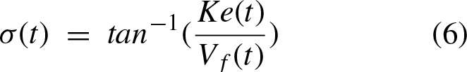
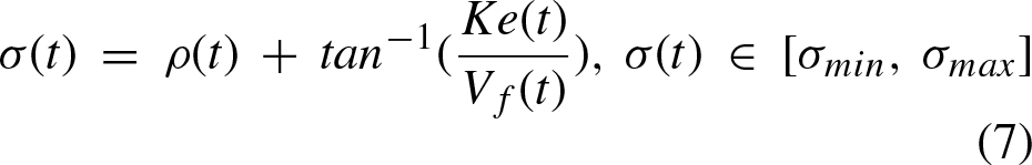
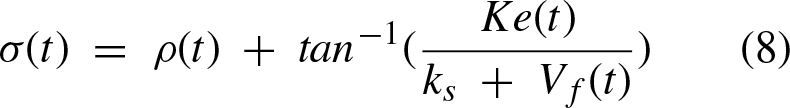
For the computation of the steering angle, as shown in [17], a constant velocity assumption is made. Given that ρ is the actual path angle of the vehicle, σ is the desired angle, V_f is the directional angle, e measures the distance from the front axle to the path, and L is the distance between the axles. The first step is to cancel the error between the actual path and the desired path, which is done by the following expression

σ (t) = ρ (t)

(5)

Then, the lane crossing error is eliminated by finding the closest point between the traced trajectory and the center of the vehicle’s front axle, denoted by e (t) in the subsequent expression:

σ (t) = \tan^{- 1} (\frac{Ke (t)}{V_{f} (t)})

(6)

where K is the gain and σ is the corrected angle of the vehicle, but this angle must be restricted to the maximum turning angles, i.e. σ (t) ∈ [σ_min, σ_max]. This leads us to the following expression:

σ (t) = ρ (t) + \tan^{- 1} (\frac{Ke (t)}{V_{f} (t)}), σ (t) \in [σ_{\min}, σ_{\max}]

(7)

Another gain k_s can be added to smooth the control and ensure that the denominator is not zero, as shown in the following expression:

σ (t) = ρ (t) + \tan^{- 1} (\frac{Ke (t)}{k_{s} + V_{f} (t)})

(8)

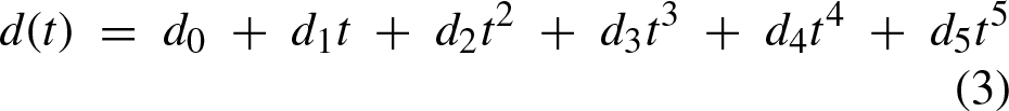
The trajectory planner produces an array denoted as δ, comprising columns representing the parameters [d, s, α, v, a]. Herein, d encapsulates the points along the lateral axis, s signifies points along the longitudinal axis, α denotes the steering angle at each point, calculated relative to the initial states, target state, and lateral deviation. v denotes the velocity, while a represents the acceleration for each point constituting a row within δ. The algorithm delineating the aforementioned process is expounded below:

Algorithm 1 Trajectory generator with Frenet frame.

Require $γ (t), [ψ_{0}^{1}, ψ_{0}^{2}, . . ., ψ_{0}^{n}], [ψ_{f}^{1}, ψ_{f}^{2}, . . ., ψ_{f}^{n}]$ ⊳ γ (t) Parametric curve of the road, $ψ_{0}^{n}$ and $ψ_{f}^{n}$ initial and target states.

Ensure:δ = [d, s, α, v, a] ⊳ Array of the way-points of the generated trajectory.

$T \leftarrow \frac{γ^{'} (t)}{{| | γ^{'} (t) | |}_{2}}$ ⊳ Vector T as longitudinal axis for the reference frame.

$N \leftarrow \frac{T^{'} (t)}{{| | T^{'} (t) | |}_{2}}$ ⊳ Vector N as lateral axis for the reference frame.

d (t) = d₀ + d₁t + d₂t² + d₃t³ + d₄t⁴ + d₅t⁵ ⊳ Lateral displacement points.

s (t) = s₀ + s₁t + s₂t² + s₃t³ + s₄t⁴ + s₅t⁵⊳ Longitudinal points.

α ← σ (t) ⊳ The steering angle comes from equations 5 to 8.

v ← s′ (t) ⊳ Velocity comes from the first derivative of the equation 3.

a ← s″ (t) ⊳ Acceleration comes from the second derivative of the equation 3. δ = [d, s, α, v, a]

3 Enhancements and compressed information approach

In a previous study [1], the Technique for Order of Preference by Similarity to Ideal Solution (TOPSIS) proposed by Alaoui in [3] served as a multicriteria decision-making method. TOPSIS evaluates the similarity of candidates to an ideal solution, determined by both an ideal worst and an ideal best for each criterion considered in the evaluation. This technique necessitates a weight vector W as a preference indicator for each column in the array γ, wherein values can range from [1, ∞]. Additionally, an influence vector I is utilized, encapsulating indicators of human preference towards either increasing or decreasing the values of the corresponding columns. To provide a comprehensive understanding of the TOPSIS technique, the ensuing algorithm elucidates the detailed process for calculating the ’Score’ assigned to each candidate. Subsequently, the trajectory with the highest ’Score’ is selected as the one deemed most fitting for the given situation.

Algorithm 2 TOPSIS applied to evaluate trajectories.

Require:Γ_ij, ⊳ Trajectories array Γ.

W_j = [w₁, . . . , w_n] ⊳ Weight vector W.

I_j = [i₁, . . . , i_n] ⊳ Impact vector I.

EnsureScore ⊳ A number between [0, 1].

$N_{Γ_{ij}} = {∥ Γ_{ij} ∥}_{2} = \sqrt{\sum_{i = 1}^{n} \sum_{j = 1}^{n} {(x_{ij})}^{2}}$ Normalization of the array.

For i in N_Γ_ido

For j in W_jdo

State W_Γ_ij ← N_Γ_ij * W_j ⊳ Applied weight to the normalized array.

end forend forifi_j =“ + ″then⊳ For wanted increase in one parameter.

I_{B
_j} = max (N_Γ_j) ⊳ I_{B
_j} Ideal best.

I_{W
_j} = min (N_Γ_j)⊳ I_{W
_j} Ideal worst.

else ⊳ For wanted decrease in one parameter.

I_{B
_j} = min (N_Γ_j)

I_{W
_j} = max (N_Γ_j)

end if $p_{d} \leftarrow \sqrt{\sum_{i = 1}^{n} (I_{B_{j}} - {N_{Γ}}_{ij})^{2}}$ ⊳ Find the positive euclidean distance between I_{B
_j} and the values on N_Γ_ij.

$n_{d} \leftarrow \sqrt{\sum_{i = 1}^{n} (I_{W_{j}} - {N_{Γ}}_{ij})^{2}}$ ⊳ Find the negative euclidean distance between I_{W
_j} and the values on N_Γ_ij.

Score ← n_d/(n_d + p_d) ⊳ Resulting Score for each Γ_irows.

As depicted in Algorithm 2, only three criteria were taken into account in the decision-making process: average speed, top acceleration, and steering angle. Despite the satisfactory results obtained, it is necessary to incorporate additional criteria for a more informed decision-making process. In this study, it was decided to include four additional parameters:

–
Rv_d The distance from the ego vehicle to the rear vehicle this can be obtained from the next expression where it is applied the euclidean distance:
${Rv}_{d} = \sqrt{(d_{v 1} - s_{v 1})^{2} + (s_{v 2} - s_{v 2})^{2}}$
(9)
where d_vn correspond to the position of the vehicle n in the axis d and s_vn is the position of the vehicle n in the lateral axis s.
–
P_c The relative position of the vehicle to the center of the lane, this cab be computed by the difference between the coordinates of the front axle center and the center of the lane. This value it is obtained from the following expression:
$P_{c} = \sqrt{(s_{V} - s_{CL})^{2}}$
(10)
where s_V correspond to the position of the vehicle n in the axis s and s_CL is the center of the lane in the lateral axis s.
–
B_d The emergency break gap relative to the speed of the vehicle, this value can be obtained from the following equation:
$B_{d} = \frac{v^{2}}{2 \cdot a}$
(11)
where v is the maximum speed of the vehicle, the calculated gap can adjust the stopping distance to the lower speeds in the trajectory, and a is the deceleration. For this work, a constant deceleration value of -5m/s² is assumed, which means that the car’s braking system can slow the car down at a rate of 5 meters per second squared.
–
LC The number of lane changes made by the trajectory generated, this value was obtained from the coordinates of the vehicle.

In the previous work, the values of the acceleration and velocity criteria were condensed to a representative value using the mean value. It was observed that employing this method significantly impacts the decision-making process, as it fails to fully capture the behavior of these criteria along the trajectory.

Therefore, there arose a necessity for a method capable of compressing the generated data without sacrificing information loss. In this study, alternative techniques were chosen for this purpose, with the prerequisite that these techniques should entail a low computational cost to augment overall performance.

In the case of acceleration, it was necessary to quantify the changes in acceleration to achieve a more comfortable ride. With this constraint, the objective was to measure the extent of changes in acceleration between the beginning and end of the trajectory.

The process commences by identifying the median value from the array δ of acceleration values, signifying the central point. Subsequently, the absolute differences between each value and this median are computed. These differences collectively indicate the degree of deviation from the center. The average of these absolute differences quantifies the overall spread of the points. To provide a meaningful scale, a desired range of 0 to 10 is established.

By employing min-max scaling, the average absolute difference is transformed to align with this predefined range. This procedural step ensures uniformity and facilitates interpretation. The resultant value is then showcased, signifying the normalized average absolute difference within the designated scale. This presentation offers insights into the distribution of points around the central value. Subsequently, this value is incorporated into TOPSIS as the criterion △a.

For the velocity criterion, the maximum value, $\max_{v}$ , is determined in relation to all the values generated in the trajectory. This value is also utilized to compute the braking gap B_d. Collectively, these criteria provide the essential information for evaluating different trajectories while ensuring safety and comfort.

The solution framework is shown in Fig. 1.

Fig. 1
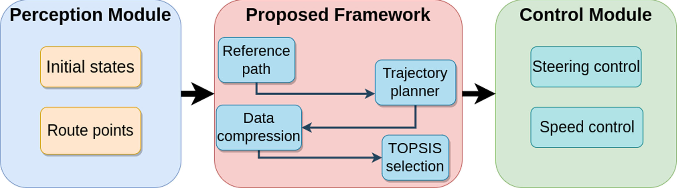
Diagram of the proposed solution framework.

Fig. 2
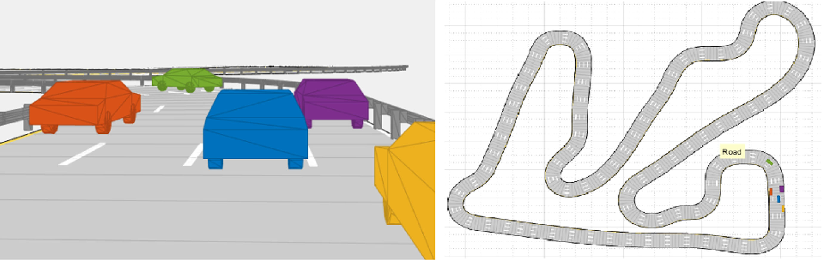
Designed scenario for the experiments.
4 Experimentation

The simulations for the experiments were conducted using the Automated Driving Toolbox in Matlab R2021a, on a computer with the following specifications: CPU Ryzen 5 3.6 GHz, 12 threads; GPU RX590 with 8 GB VRAM and 16 GB of RAM, equipped with a 1 TB SSD. The scenario, illustrated in Fig. 2, consists of a road with winding and straight segments, featuring four lanes of 2 meters each, simulating a highway. The scenario does not include crossings, intersections, or junctions.

The simulation involved four non-controllable vehicles with dimensions identical to the controlled vehicle, following a predetermined path that included lane-changing and lane-keeping maneuvers. The controlled vehicle, or ego vehicle, traversed the path from a start point to a target point and possessed the following characteristics: length = 4.7 meters, width = 1.8 meters, and a rear axle ratio of 0.25.

The experiments involved testing three sets of weight W and impact I vectors, tailored to three distinct driving styles. These vector sets were derived from data collected from human drivers, aiming to mirror the transfer of experience to the decision-making system.

A conservative style was considered, aiming to emulate a cautious driver who prefers to maintain a low speed, avoids complicated maneuvers, and remains in their lane unless absolutely necessary for overtaking. The second style, moderate, simulates a more experienced yet cautious driver with a propensity to increase speed while prioritizing passenger comfort. This driver refrains from executing risky maneuvers and changes lanes only when essential. Lastly, an aggressive style emulates a driver inclined to accelerate, undertake risky maneuvers without much concern for passenger comfort, and frequently change lanes to advance at higher speeds. The values for each vector are presented in Table 1.

Table 1
Values for vectors W and I for each driving style

Driving style Vectors $\max_{v}$ △a α Rv _d P _CL B _d LC

Conservative W 2 5 3 3 5 5 4

I – – – + – + –

Moderate W 2 3 2 3 5 4 3

I – – – + – + –

Aggressive W 3 4 3 2 3 3 2

I + + + – – – –

Driving style	Vectors	$\max_{v}$	△a	α	Rv _d	P _CL	B _d	LC
Conservative	W	2	5	3	3	5	5	4
	I	–	–	–	+	–	+	–
Moderate	W	2	3	2	3	5	4	3
	I	–	–	–	+	–	+	–
Aggressive	W	3	4	3	2	3	3	2
	I	+	+	+	–	–	–	–

The additional methods employed for comparison included Long Short-Term Memory (LSTM) [15]. The chosen LSTM model utilizes the NGSIM database [18] and formulates trajectories to prevent collisions. Another method involved a Reinforcement Learning model, specifically a Deep Q-learning Network (DQN) [13], trained on the same dataset to formulate policies for decision-making on highways. These models were further benchmarked against the version of TOPSIS utilized in [1].

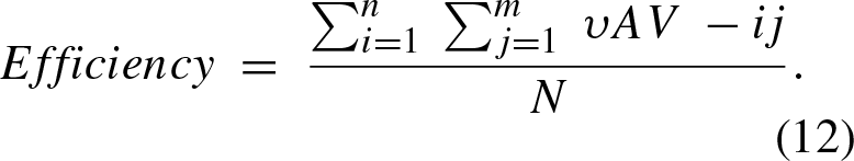
The metrics that were used to measure the performance of the models were as follows: –

Efficiency, denoted as the average longitudinal speed of the autonomous vehicle and the rest of the vehicles in the scenario, through this metric the efficiency of the controlled vehicle and the relative speed of the whole traffic flow can be evaluated with the following functions:

Efficiency = \frac{\sum_{i = 1}^{n} \sum_{j = 1}^{m} υ AV - ij}{N} .

(12)

Efficiency = \frac{\sum_{i = 1}^{n} \sum_{j = 1}^{m} υ ij}{N_{all}} .

(13)

where υAV - ij represents the longitudinal velocity of trajectory i at time j. υij is the longitudinal velocity of vehicle i at time j. N is the total number of trajectories, considering that each one has a different velocity for each time instant. N_all indicates the total number of velocities for all vehicles at all time instants.

–

Safety, a collision percentage was defined as the probability that the vehicle will collide in each trajectory, this probability is expressed in the following expression:

Safety = \frac{N_{colision}}{N_{NCV}} .

(14)

where N_collision is the number of paths with collisions in each process, N_NCV represents the number of obstacles with which an interaction is had.

–

Comfort, trough measuring the acceleration changes in each selected trajectory, contemplating that an acceleration change could be denoted in the following range (-4.5 s^-2, 4.5 s^-2) in an absolute range of [0, 1].

–

Lane Change Frequency and Quality Index (LCFQI), metric is made up of two main components: Lane Change Frequency (LCF) measures how often a self-driving vehicle changes lanes, based on the raw number of lane changes; Lane Change Quality (LCQ) evaluates the smoothness, safety, and appropriateness of each lane change, with sub components including Smoothness (S), which measures the quality of the transition; Safety (S_a), which evaluates compliance with safety rules; and Appropriateness (A_p), which measures the necessity and sensitivity of lane changes.

LCFQI = (α \cdot LCF) + (β \cdot LCQ) .

(15)

where τ and β are weight factors that determine the relative importance of frequency and quality.

LCQ = w_{s} \cdot S + w_{sa} \cdot S_{a} + w_{ap} \cdot A_{p} .

(16)

Where S denotes the smoothness component, S_a denotes the safety component, A_p represents the adequacy component, w_s, w_sa, and w_ap are weight factors for each subcomponent, respectively.

5 Results and discussion

In this section, we assess the performance of the proposed framework and juxtapose the results with other methods, namely LSTM, DQN, and Non-enhanced TOPSIS (NeTOPSIS). The experiments mentioned earlier involved each model undergoing fifty iterations in the given scenario.

The study revealed that distinct driving styles yielded varying outcomes. The conservative style maintained speeds below 15km/h, predominantly adhered to one lane, and exhibited minimal lane changes, resulting in reduced comfort and occasional rear-end collisions. The moderate style, with speeds below 35km/h, executed calculated lane changes, prioritized comfort, and experienced fewer collisions. On the other hand, the aggressive style reached speeds up to 50km/h, executed the most lane changes, encountered more collisions, and diminished comfort due to abrupt actions. The NeTOPSIS style closely resembled the conservative style but deviated off the road more frequently at 30km/h and displayed shortcomings in curve smoothness and stopping distance.

Regarding the speed, there is a significant distinction between the Conservative style and the other two styles, with NeTOPSIS falling between Conservative and Moderate. Figure 3 illustrates the average top speed of the vehicle across all iterations.

Fig. 3

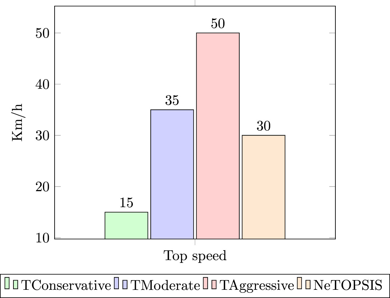
Average top speed.

The collision analysis over the total number of iterations indicates that the driving style with the highest safety was Moderate, followed by Conservative, while Aggressive exhibited the worst performance after NeTOPSIS, as depicted in Fig. 4, which illustrates the values for each model across a total of 50 iterations.

Fig. 4

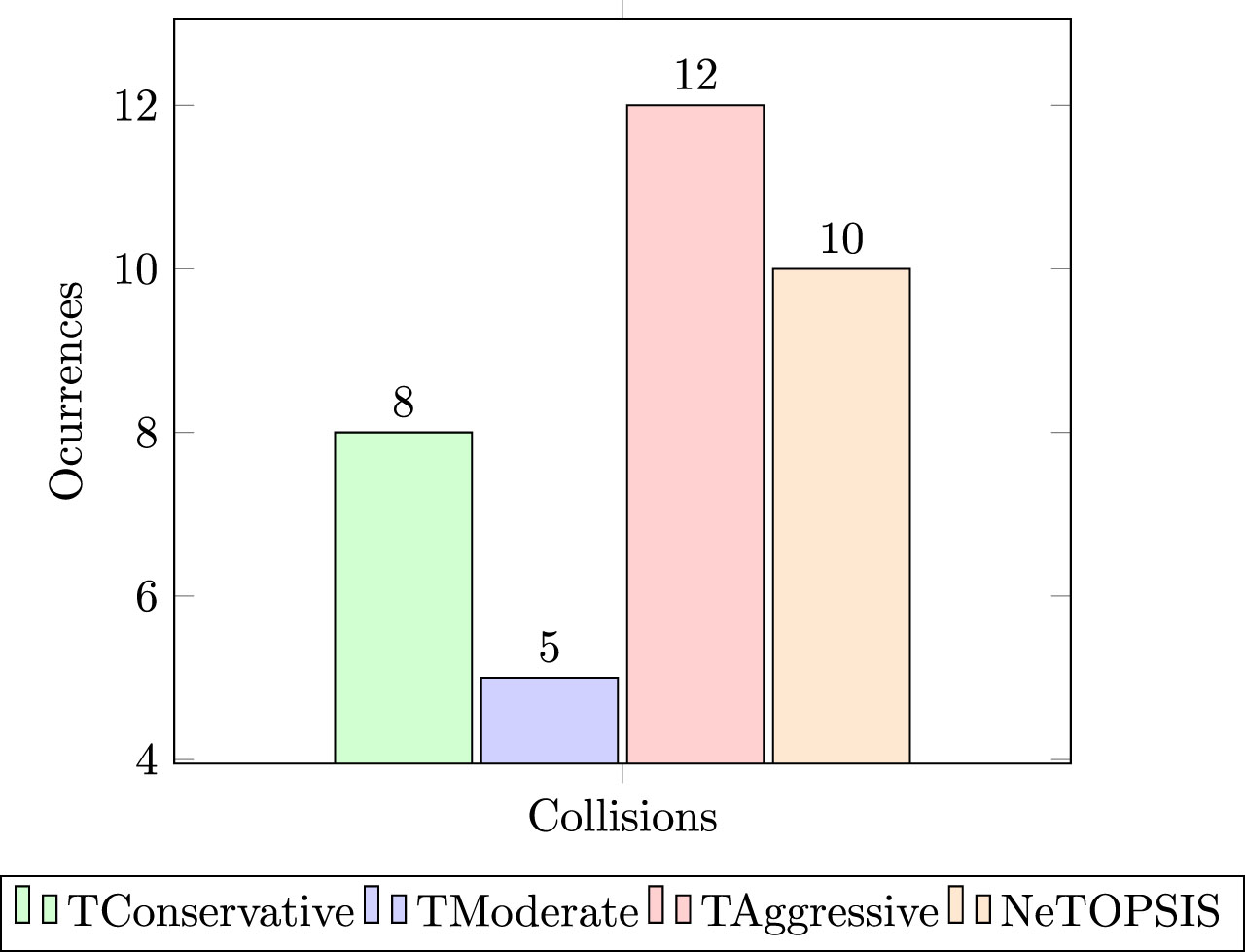
Number of iterations with collisions.

The models demonstrate divergent speed-comfort relationships, with lower values indicating greater comfort. The Conservative model maintains stable high comfort across a broad speed range, with a slight decline at higher speeds. The Moderate model starts with consistently high comfort, slightly decreasing as speed rises. The Aggressive model exhibits an inverse trend, with comfort dropping as speed increases, with a milder decline at higher speeds. NeTOPSIS begins with moderate comfort, decreasing slightly with speed and more significantly as speed rises. These outcomes highlight varied speed-comfort interactions across models, as illustrated in Fig. 5.

Fig. 5

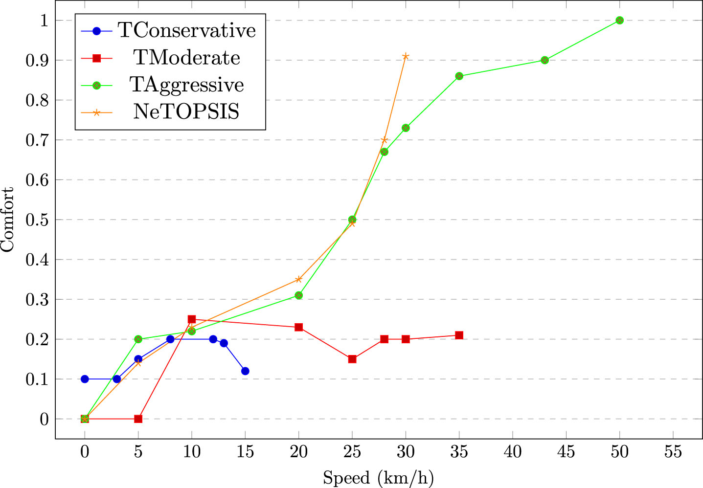
Comfort of each model.

Figure 6 presents a comparison between the number of lane changes for the three driving styles and NeTOPSIS. The number of maneuvers aligns with the configuration of the vectors W and I.

Fig. 6

Lane changes in relation to speed.

The performance of the models is evaluated based on several criteria. In terms of efficiency, the Conservative (CON) TOPSIS model achieves the lowest speed at 15, Moderate (MOD) performs at 35, Aggressive (AGG) reaches 50, NeTOPSIS reaches 30, LSTM achieves 42, and DQN reaches 38. Safety is measured by the number of safety violations, and among the TOPSIS models, Moderate has the fewest with 5, while Aggressive has the highest with 12. NeTOPSIS shows a safety score of 10. Comfort, where lower values indicate higher comfort, shows that Conservative scores 0.12, Moderate 0.23, Aggressive reaches 1, and NeTOPSIS stands out with a value of 0.91. When these factors are combined into the Lane Change Frequency and Quality Index (LCFQI), Aggressive scores the highest at 18.88, followed by NeTOPSIS at 15.57 and Moderate at 9.57. LSTM scores 10.22, and DQN scores 9.38. Overall, these scores represent different behaviors among the models, with Aggressive prioritizing efficiency at the expense of safety and comfort, NeTOPSIS balancing safety and comfort with reasonable efficiency, and Moderate leaning toward safety and comfort while maintaining moderate efficiency. LSTM and DQN have similar LCFQI scores, demonstrating a balance between the metrics. As shown in Table 2.

Table 2

Comparative results of the models and driving styles.

		Efficiency	Safety	Comfort	LCFQI
TOPSIS	CON	15	8	0.12	2.28
	MOD	35	5	0.23	9.57
	AGG	50	12	1	18.88
NeTOPSIS		30	10	0.91	15.57
LSTM		42	9	0.3	10.22
DQN		38	7	0.28	9.38

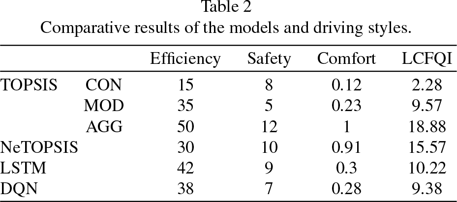
Comparing the TOPSIS Moderate model with the LSTM and DQN models reveals significant differences in various evaluation criteria. In terms of efficiency, LSTM has about a 20% lower efficiency than Moderate, while DQN lags behind by about 8.57%. Regarding safety, LSTM experiences a significant 80% increase in safety violations compared to Moderate, while DQN has 40% more violations. Comfort levels indicate that both LSTM and DQN have higher discomfort levels, with LSTM being approximately 30.43% less comfortable and DQN being approximately 21.74% less comfortable than Moderate. When evaluating the overall Lane Change Frequency and Quality Index (LCFQI), LSTM slightly outperforms Moderate by about 6.78%, while DQN’s LCFQI falls about 1.99% below Moderate’s. These results underscore the distinct differences in performance between the models and indicate the areas in which each model excels or lags.

The obtained results align with the anticipated behavior of the adjusted TOPSIS model. It is crucial to acknowledge that, in contrast to other methods, refining the influence and weight vectors for a reduced feature set yields some improvement in accuracy. Expanding the scope to include more parameters has the potential to enhance lane maintenance and accommodate a dynamic speed range. The differentiating factor between the proposed model and conventional techniques lies in its augmented decision-making capability, leading to more streamlined execution times. Unlike standard trajectory selection methods, the proposed approach considers a broader range of decision-influencing factors, irrespective of the trajectory generation method. This inherent flexibility allows seamless integration, enabling input from various sensors or trajectory planners without inflating computational requirements. The decision paradigm, characterized by its human-like features inherited through the transfer of experience and data analysis via importance and preference, complements the enhanced perceptual capabilities of autonomous systems.

6 Conclusion and future work

For this study, trajectories were generated using fifth and fourth-order polynomials. The data produced by this path planning algorithm were then compressed using various statistical methods to provide a more concise description of the generated trajectory. Additionally, new criteria were considered for the decision-making process. The flexibility of TOPSIS allowed for scalability and easy integration of human experience to accommodate these new criteria.

The experiments for this research were conducted using the Automated Driving Toolbox in Matlab R2021a. The dynamic scenario simulated a four-lane road and did not include any perception techniques, as they were not the focus of the research. The scenario aimed to replicate highway conditions with straight and sinuous road segments. The presence of dynamic obstacles, such as other vehicles traveling on the same road, added complexity to the path planning task.

In summary, the performance evaluation of the models encompassed various criteria. The Conservative (CON) TOPSIS model exhibited the lowest speed at 15, Moderate (MOD) operated at 35, Aggressive (AGG) reached 50, and NeTOPSIS reached 30. In terms of efficiency, LSTM and DQN achieved speeds of 42 and 38 respectively. Safety assessments indicated that among the TOPSIS models, Moderate had the fewest safety violations with 5, while Aggressive had the highest with 12, and NeTOPSIS scored 10 in safety. Comfort assessments, where lower values indicate better comfort, ranked Conservative at 0.12, Moderate at 0.23, Aggressive at 1, and NeTOPSIS at 0.91. Combining these factors into the Lane Change Frequency and Quality Index (LCFQI), Aggressive led with 18.88, followed by NeTOPSIS with 15.57, Moderate with 9.57, LSTM with 10.22, and DQN with 9.38.

Notably, Aggressive prioritized efficiency over safety and comfort, NeTOPSIS balanced safety and comfort with reasonable efficiency, and Moderate leaned toward safety and comfort with moderate efficiency. Comparisons with LSTM and DQN revealed significant differences across all criteria, with LSTM showing about 20% less efficiency and 80% more safety violations than Moderate, and DQN showing about 8.57% less efficiency and 40% more safety violations. In terms of comfort, both LSTM and DQN experienced higher discomfort, being about 30.43% and 21.74% less comfortable than Moderate, respectively. While LSTM slightly outperformed Moderate by about 6.78% on the LCFQI, DQN fell about 1.99% below Moderate’s score. These differences underscore the distinct performance disparities between the models and highlight their respective strengths and weaknesses.

The introduction of new criteria and a more precise method of compressing the generated data, without sacrificing representativeness, contributes to achieving performance comparable to more sophisticated methods such as Deep Learning or Reinforcement Learning. Additionally, this technique does not necessitate large datasets or extensive training phases, making it a valid alternative considering the performance-to-computational-cost ratio. In a sense, it can be viewed as an alternative version of Reinforcement Learning, guided by a reward function to exhibit a bias toward certain behaviors. In the case of TOPSIS, this is accomplished by adjusting the weight and importance vectors, with the significant advantage of immediate implementation. While it is acknowledged that in some cases, other methods might outperform TOPSIS, it’s essential to note that only six parameters were considered, leaving room for further improvement.

For future work, there is a consideration for enhancing the technique itself to facilitate more direct integration within the trajectory planner. This is aimed at improving the response time of the algorithm. Additionally, the exploration of new criteria is contemplated to enhance the technique’s performance, particularly at higher speeds. Beyond that, there is a plan to implement the technique in a scale model to observe its behavior under real-world conditions. This real-world implementation could provide valuable insights into the practical applicability and effectiveness of the proposed approach.

Footnotes

Acknowledgments

The authors thank CONAHCYT, as well as TecNM-CENIDET for their financial support.

References

Arenas Muñiz

A.A.

, Mújica Vargas

Rendon Castro

Luna Álvarez

, Topsis method for multiplecriteria decision-making applied to trajectory selection for autonomous driving, In Mexican Conference on Pattern Recognition, pages 295–307. Springer, 2023.

Bakioglu

Atahan

A.O.

, Ahp integrated topsis and vikor methods with pythagorean fuzzy sets to prioritize risks in self-driving vehicles, Applied Soft Computing99 (2021), 106948.

El Alaoui

, Fuzzy TOPSIS: Logic, Approaches, and Case Studies, CRC Press, 2021.

Gao

Liu

Yang

Luan

, Multi-agent decision-making modes in uncertain interactive traffic scenarios via graph convolution-based deep reinforcement learning, Sensors22(12) (2022), 4586.

Hang

Xing

Huang

, Human-like decision making for autonomous driving: A noncooperative game theoretic approach, IEEE Transactions on Intelligent Transportation Systems22(4) (2020), 2076–2087.

Yang

, Robust lane change decision making for autonomous vehicles: An observation adversarial reinforcement learning approach, IEEE Transactions on Intelligent Vehicles 2022.

Hoel

C.-J.

Driggs-Campbell

Wolff

Laine

Kochenderfer

M.J.

, Combining planning and deep reinforcement learning in tactical decision making for autonomous driving, IEEE Transactions on Intelligent Vehicles5(2) (2019), 294–305.

Hoel

C.-J.

Wolff

Laine

, Tactical decision-making in autonomous driving by reinforcement learning with uncertainty estimation, In 2020 IEEE Intelligent Vehicles Symposium (IV), pages 1563–1569. IEEE, 2020.

Wang

Ren

Khajepour

, Path planning and tracking for vehicle collision avoidance in lateral and longitudinal motion directions, Synthesis Lectures on Advances in Automotive Technology Synthesis Lectures on Advances in Automotive Technology, 2021.

10.

Yang

Lyu

S.E.

, Decision making of autonomous vehicles in lane change scenarios: Deep reinforcement learning approaches with risk awareness,, Transportation Research Part C: Emerging Technologies134 (2022), 103452.

11.

Liao

Liu

Tang

Huang

Cao

, Decision-making strategy on highway for autonomous vehicles using deep reinforcement learning,, IEEE Access8 (2020), 177804–177814.

12.

Moghadam

Elkaim

G.H.

, A hierarchical architecture for sequential decision-making in autonomous driving using deep reinforcement learning, arXiv preprint arXiv:1906.08464, 2019.

13.

Mohammadhasani

Mehrivash

Lynch

Shu

, Reinforcement learning based safe decision makingfor highway autonomous driving, arXiv preprint arXiv:2105.06517, 2021.

14.

Shen

Chen

Cao

Yang

S.X.

, An improved deep network-based scene classification method for self-driving cars,, IEEE Transactions on Instrumentation and Measurement71 (2022), 1–14.

15.

Shi

Fan

Wang

Yin

, A novel network architecture of decision-making for self-driving vehicles based on long short-term memory and grasshopper optimization algorithm,, IEEE Access8 (2020), 155429–155440.

16.

Shu

Chen

Wang

Cao

, Autonomous driving at intersections: A behavior-oriented critical-turning-point approach for decision making, IEEE/ASME Transactions on Mechatronics27(1) (2021), 234–244.

17.

Sorniotti

Barber

Pinto

S.D.

, Path tracking for automated driving: A tutorial on control system formulations and ongoing research, Springer International Publishing, 1 2016.

18.

Thompson

, Next generation simulation (ngsim) vehicle trajectories and supporting data, Data set, 2022.

19.

Wang

Talbot

Gerdes

J.C.

Schwager

, Game-theoretic planning for self-driving cars in multivehicle competitive scenarios, IEEE Transactions on Robotics37(4) (2021), 1313–1325.

20.

Wang

Jiang

Lin

Fang

Meng

, Imitation learning based decision-making for autonomous vehicle control at traffic roundabouts, Multimedia Tools and Applications81(28) (2022), 39873–39889.

21.

Wang

Qie

Yang

Liu

Xiang

Huang

, An intelligent lane-changing behavior prediction and decision-making strategy for an autonomous vehicle, IEEE Transactions on Industrial Electronics69(3) (2022), 2927–2937.

22.

Zhang

Ogai

Inujima

Tateno

, Tactical decision-making for autonomous driving using dueling double deep q network with double attention,, IEEE Access9 (2021), 151983–151992.

Optimized TOPSIS technique for trajectory selection of self-driving vehicles on highways

Abstract

Keywords

1 Introduction

2 Trajectory planning

Table 1 Values for vectors W and I for each driving style Driving style Vectors max v △a α Rv d P CL B d LC Conservative W 2 5 3 3 5 5 4 I – – – + – + – Moderate W 2 3 2 3 5 4 3 I – – – + – + – Aggressive W 3 4 3 2 3 3 2 I + + + – – – –

Footnotes

Acknowledgments

References

Table 1
Values for vectors W and I for each driving style

Driving style Vectors $\max_{v}$ △a α Rv _d P _CL B _d LC

Conservative W 2 5 3 3 5 5 4

I – – – + – + –

Moderate W 2 3 2 3 5 4 3

I – – – + – + –

Aggressive W 3 4 3 2 3 3 2

I + + + – – – –