A mathematical model of temperature distribution along the length of the oil production well

Abstract

The paper gives a systems analysis in the field of heat transfer and temperature distribution (TD) along the length of oil production wells (OPW). The analysis shows that the existing mathematical models are suitable only for determining TD along the length of casing string (CS) and are not suitable for determining TD along the length of the tubing run, since the existence of the interfacial (between the CS and the tubing) annulus of the fluid and gas layers with heat capacity and thermal conductivity that differ significantly from the heat capacity and thermal conductivity of rocks surrounding the CS. Given the above, mathematical models taking into account the impact of the fluid and gas layers in the annulus on the heat transfer from the upward fluid flow to the tubing wall and from the wall to the interfacial annulus are developed. To ensure the technological effectiveness of the obtained model, formulas for quantitative estimation of the heat transfer of the fluid flow into the surrounding environment are given.

Keywords

Heat exchange heat transfer heat dissipation thermal conductivity temperature distribution oil production well.

1 Introduction

Numerous studies are devoted to the issues of operating temperatures of oil production wells (OPW), addressing various aspects of this complex phenomenon [1–8]. In particular, these studies propose mathematical formulas for determining the temperature distribution along the length of the production (casing) string and the tubing. It is noted in [9, 10] that the formation of asphaltene-resin-paraffin deposits (ARPD) on the surface of down hole equipment, the tubing, and the CS is one of the main causes complicating the process of OPW operation. Wong H. has a monograph published as a reference book on the effects of thermal conductivity and heat transfer in heat exchange processes [12]. This reference book gives the most complete number of ratios and values in the form of formulas, tables, and graphs, which are convenient for calculating specific heat transfer cases. Essentially all the main types of heat transfer are considered in it: thermal conductivity, convective, and radiation heat transfer. It is shown that the proposed data can be used to estimate the efficiency of heat transfer between a fluid and a solid wall. The given formulas make it possible to determine the efficiency of heat exchange apparatuses.

Since it is difficult to calculate the heat transfer accurately, it is determined by a simplified law. Newton’s law of cooling, according to which the amount of heat dQ, released by a surface element dF with a temperature t_w into the environment with a temperature t_f over time dτ, is directly proportional to the temperature difference (t_w - t_f) and the values of dF and dτ [11, 13], is used as the basic heat transfer:

dQ = \propto (t_{w} - t_{f}) dFd τ

(1)

and at a steady state of the heat transfer process, when the fluid and wall temperature remain unchanged

Q = \propto (t_{w} - t_{f}) F τ kcal

(2a)

where ∝ is the coefficient of proportionality, which is determined experimentally, called the heat transfer coefficient.

To describe convective heat transfer, the Fourier-Kirchhoff equation or differential equation of heat conduction in a moving medium is given in [14]:

ω_{x} \frac{\partial t}{\partial x} + ω_{y} \frac{\partial t}{\partial y} + ω_{z} \frac{\partial t}{\partial z} = a (\frac{\partial^{2} t}{\partial x^{2}} + \frac{\partial^{2} t}{\partial y^{2}} + \frac{\partial^{2} t}{\partial z^{2}})

(3)

where

α = \frac{λ}{C_{p} ρ}

is the thermal diffusivity of the fluid, m²/h; c_P is the specific heat capacity of the fluid, kcal/ (kg. ⁰C); ρ is the density of the fluid, kg/m³.

In this equation, the other variables besides temperature are the velocity and density of the fluid, and therefore it describes different aspects of the convective heat transfer process.

The impossibility of an analytical solution of equations of motion and convective heat transfer (2) forces one to resort to a similar transformation of the system of these equations and present them as some function of dimensionless numbers (DN). These DNs will characterize all factors affecting convective heat transfer processes.

Classical scientists such as Traskov, Reynolds, Prandtl, Nusselt, Gretz, Stanton, and Peclet were engaged in the development of such DNs [15]. In particular, the English scientist O. Reynolds studied the process of heat transfer when a fluid moves through pipes. He noticed that at a given temperature difference the heat transfer depends on the so-called fluid diffusion near the surface of the walls. The mechanism by which heat transfer is accomplished in the fluid is identical to the mechanism by which internal friction is accomplished.

Both phenomena depend solely on the nature of fluid motion and are carried out by the same agent, the moving fluid particles.

Hence the basic Reynolds’ law of heat transfer: the ratio of heat transferred to the pipe walls by convection (Latin: carrying, conveying), i.e., the transfer of heat with the moving medium over all the heat that could be taken away by the fluid from the walls, equals the ratio of the amount of motion lost by the fluid due to surface friction to the total amount of fluid motion [16].

Stanton and Taylor had an essential addition to Reynolds’s theory. They noticed that in turbulent mode a very thin boundary layer forms near the pipe walls, in which the motion is purely laminar (i.e., jet motion discovered by Poiseuille); at the same time this layer generates vortices and sends them to the rest of the fluid mass, where they move fluid particles, due to which almost the same flow velocity is obtained here. This central region of the flow in the pipe, which occupies almost the entire cross-section of the pipe, is called the flow core (which possesses a constant velocity).

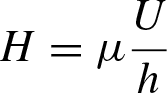
The value of the heat transfer coefficient α in formula (1) depends on a large number of factors and is a function of several variables. First of all, the value of α is determined by the following factors: 1)

type of fluid (gas, steam, dripping liquid);

nature of the fluid flow (forced or free flow);

wall shape (linear dimensions L, d);

state and properties of the fluid (temperature t_f, pressure P, density ρ, specific heat capacity c , thermal conductivity λ, viscosity μ);

motion parameters (velocity ω);

wall temperature t_w.

Thus,

\propto = f (L, d, \dots, t_{f}, P, ρ, C, λ, μ, ω, t_{w}) .

This relationship shows that the simplicity of Equation (1) is only apparent.

The dependence of ∝ on a large number of factors does not allow for a general formula to determine it, and in each particular case, it is necessary to resort to experimental studies.

Given the above factors, experimental studies to determine the values of ∝ by Stanton and Taylor produced the following formula [17].

\propto = \frac{HC}{ω [1 + \frac{4}{ω} (\frac{ω}{λ} - 1)]}

(4)

H = μ \frac{U}{h}

where U is the velocity in the boundary layer, m/h; ω is the average flow rate, m/h; h is the boundary layer thickness, m; H is the friction force per unit surface, MPa.

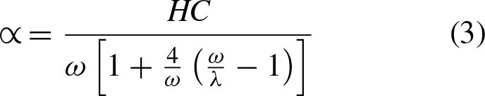
The value of the relationship S = U/ω is determined empirically. Zoenekin’s experiments with water flowing through an elongated 192 cm long, 1 cm diameter brass pipe established that the average value of U/ω = 0.3383 [Table 1]. Tan-Bosch denotes this ratio by S = 0.35. From semi-theoretical (witty) and semi-experimental considerations Taylor established that the value of S = 0.38. Academician A.S. Leibenzon as a result of theoretical considerations established that $S = \frac{1}{3} ω$ . Consequently, this conclusion is the most probable. Riege will also take a close value for S = 1/3 : 0.33 S < 0.34.

The heat transfer coefficient at forced turbulent flow in a straight circular tube, in particular in the CS and the tubing can be determined by the expression [12].

NU = f (Re, \Pr, \frac{l}{l_{0}})

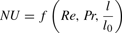
When processing the experimental data, the researchers obtained various calculation formulas. The most reliable results are given by the following formula for both dripping liquids (oil and water) and gases [12].

Nu = 0, 023 {Re}^{0.8} P_{r}^{0.4},

(5)

from which it follows that:

\propto = 0, 023 \frac{λ}{d} {Re}_{0, 8} {Pr}^{0, 4}, kcal/ (m .^{2} h .^{0} C)

(6a)

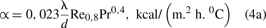
where Nu =∝ d/λ is the Nusselt number; $R e = \frac{ρ ω d}{μ}$ is the Reynolds number; $\Pr = \frac{μ C_{P}}{λ}$ is the Prandtl number; c_P is the specific heat capacity at constant pressure, kcal/(kg. ⁰C).

It follows from the above that the value of the heat transfer coefficient can be determined with a sufficient degree of accuracy only by empirical formulas, in particular formulas (3) and (4a).

Formula (4a) is applicable at the following values: number Re < 10000, number Pr = 0.7÷2500, wall temperature –below the boiling point of the fluid, ratio of pipe length to its diameter –l/d > 50 [12].

2 Problem statement

One of the topical problems occurring in OPW is the process of asphaltene-resin-paraffin deposits (ARPD) on the surface of the CS and the tubing, which leads to a decrease in OPW productivity and pumping unit efficiency [9, 10, 14, 19]. Another problem is intensive gas emission in the cylinder of the sucker-rod pumping unit (SRPU), installed in the lower (end) part of the tubing when the plunger moves upwards and, consequently, when the intake valve is opened. The release of gas in the pump cylinder results in an incomplete filling of the cylinder and hence a decrease in the pump performance. Among the conditions contributing to the formation of deposits are lower pressure and temperature of the upward flow in the CS and the tubing [16, 17]. It is known that the paraffin solvency of oil decreases with decreasing temperature and degassing of oil. In this case, the temperature factor prevails [14]. The intensity of heat transfer depends on the temperature of the reservoir fluid (oil, water, and gas) and the rocks surrounding the CS, as well as the thermal conductivity of the annulus between the CS and the tubing, filled with an oil-water mixture and a gas cap [18].

The practice of oilfield production shows that ARPD is deposited most heavily on the inner surface of the tubing. Besides, when reservoir fluid moves from the bottom hole to the mouth of the CS and from the depth of the pump placement to the mouth of the tubing, due to a gradual decrease in the temperature of the flow, the oil (oil emulsion) viscosity increases and, consequently, so does the hydraulic resistance (friction force) to the upward flow. Therefore, determining the law of temperature distribution of the upward fluid (oil-water mixture) flow along the length of the CS from the bottom hole to the wellhead and of the tubing from the depth of the pump placement to the wellhead is a relevant problem, that is the subject of this paper.

3 Solution

As mentioned earlier, many studies [1–8, 11, 12] are devoted to the solution of this problem. Of these studies, we can particularly highlight our previous works [20] and the works of: Chekalyuk E.B., who proposed mathematical expressions [1, p.136, eq. Vll.25] for determining the temperature distribution of upward fluid flow in the CS from the bottom hole to the mouth; Mishchenko I.T., who also proposed a mathematical model for temperature distribution along the length of OPW [8, p.317, eq. (6.120)]. However, these equations (Vll.25) and (6.120) do not allow determining temperature distribution along the length of the tubing. On this subject, it is also worth mentioning the study by Wong H. [21], where it is shown that if the value of the fluid temperature t_f1 is known for one of the cross sections of the pipeline, the value of the temperature t_f2 in another cross-section located at a distance l from the first one can be determined from the following equation [22]:

t_{f 1} = \frac{\bar{\propto} P l (2 t_{w} - t_{f 1}) + 2 U_{T} C_{p} {St}_{f 1}}{\bar{\propto} P l + 2 U_{T} C_{p}} \cdot^{0} C

where P and S are the perimeter and the cross-sectional area of the pipe, respectively; U_T is the mass velocity;

\bar{\propto}

is the the average value of the heat transfer coefficient on the length l; c_P is the specific heat capacity of the fluid at constant pressure.

To derive the formula for temperature distribution in the upward flow along the depth (length) of the CS and the tubing, we first draw up a thermal balance of temperature variation under steady-state heat transfer. The heat generated by energy consumption to overcome the viscous friction within the considered pipe section equal to (P₁-P₂)V will partially go to heating the fluid itself, due to convective heat transfer and heat conduction, to the environment, where P₁ and P₂ are pressure values at the beginning and end of the pipe section, MPa; V is the transported volume.

Consider a stationary state:

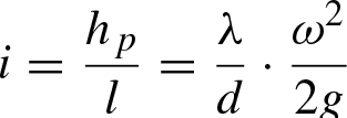
Suppose that the Z-axis is directed along the tubing axis with a diameter d. We select the tubing element 12 (Fig. 1) formed by two cross-sections 11’ and 22’ with distance dZ. If we denote by γ the specific weight, the work expended on the friction along the lift pipe (LP) of length (height) dZ is γVidZ, where i, according to the Darcy-Weisbach formula, is called the hydraulic gradient, which describes the loss of head per length of the LP:

Fig. 1

The tubing layout when the plunger is moving upward, when the discharge valve is closed, and the intake valve is open.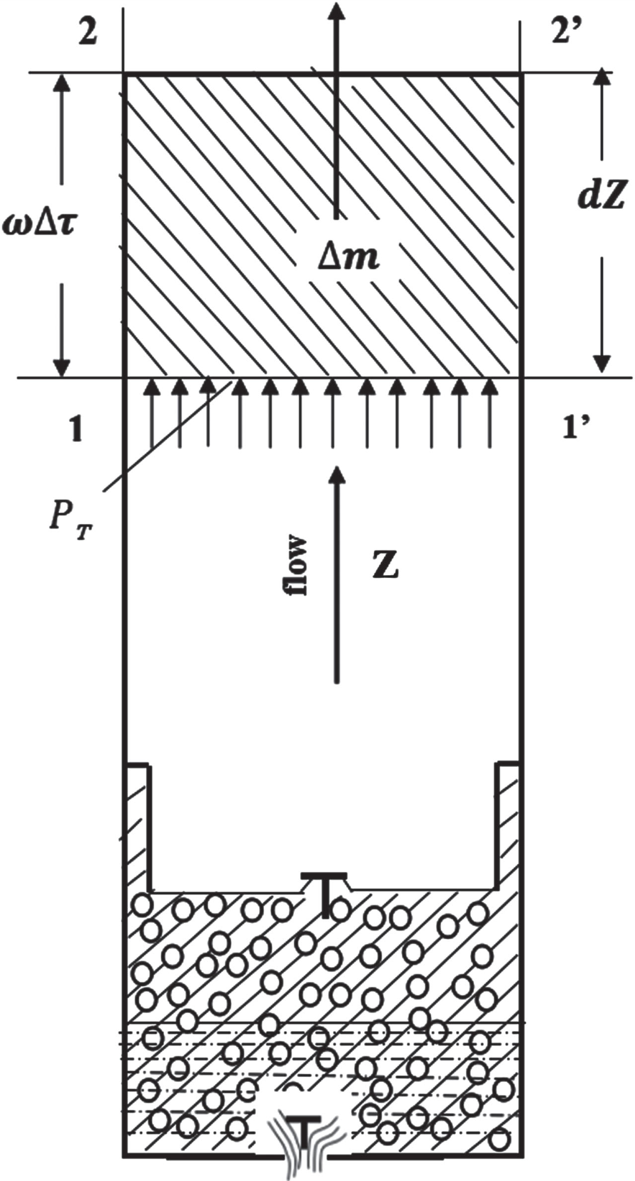

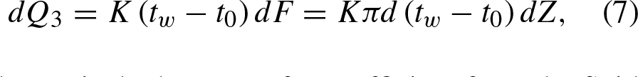
i = \frac{h_{p}}{l} = \frac{λ}{d} \cdot \frac{ω^{2}}{2 g}

where λ is the hydraulic resistance coefficient, which in the general case is a function of the Reynolds number and relative roughness. This work, as noted above, is converted into thermal energy. If we denote the amount of heat equivalent to the work produced by dQ₁, then

{dQ}_{1} = \frac{G γ i}{E} dZ

(7)

where E is the mechanical equivalent of heat, kgm/kcal; G is the fluid flow rate, m³/h. The heat loss for cooling in section 1-2 will be

{dQ}_{2} = G ρ cdt,

(8)

where c, ρ are the specific heat capacity, kcal/kg. ⁰C, and the density, kg/m³, of the fluid, respectively.

The amount of heat released in section 1-2 by the pipe wall, with a temperature t_w, into the external environment with a temperature t₀ according to Newton’s law of cooling will have the value

{dQ}_{3} = K (t_{w} - t_{0}) dF = K π d (t_{w} - t_{0}) dZ,

(9)

where К is the heat transfer coefficient from the fluid flow to the environment.

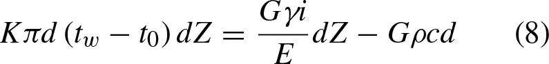
Obviously, dQ₂, lost by the fluid in section 1-2, plus the heat dQ₁ generated here by friction, will be equal to dQ₃ lost in this section from cooling

K π d (t_{w} - t_{0}) dZ = \frac{G γ i}{E} dZ - G ρ cd

(10)

- dt = a (t - t_{0} - b) dZ

where

a = \frac{K π d}{G ρ c}; b = \frac{G γ i}{K π dE} = \frac{G Δ P}{K π dEl}

(11)

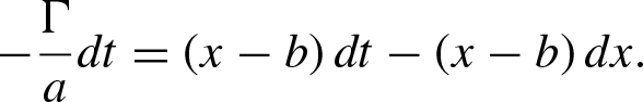
Since the environment in the upward fluid flow in the CS and the tubing is rocks, in Equation (9) instead of t₀ it is necessary to use the geometric gradient, ⁰C/m (ΓZ) (see Fig. 1). Then Equation (9) takes the following form:

- dt = a (t - Γ Z - b) dZ

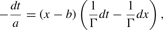
Substituting t - ΓZ = x and $dZ = \frac{1}{Γ} dt - \frac{1}{Γ} dx$

- \frac{dt}{a} = (x - b) (\frac{1}{Γ} dt - \frac{1}{Γ} dx),

therefore,

- \frac{Γ}{a} dt = (x - b) dt - (x - b) dx .

Separating the variables we obtain

(x - b + \frac{Γ}{a}) dt = (x - b) dx

\begin{matrix} dt = \frac{x - b}{x - b + \frac{Γ}{a}} dx = \frac{(x - b) + \frac{Γ}{a} - \frac{Γ}{a}}{(x - b) + \frac{Γ}{a}} dx \\ = dx - \frac{\frac{Γ}{a}}{(x - b) + \frac{Γ}{a}} dx \end{matrix}

t = x - \frac{Γ}{a} ln (x - b + \frac{Γ}{a}) + C

t = t - Γ Z - \frac{Γ}{a} ln (t - Γ Z - b + \frac{Γ}{a}) + C,

where C is arbitrary (an integral constant, which under the condition Z = H - h, where H and h are well depth (CS) and depth of the pump placement, m; at h = HZ = 0 and t = t₃ (bottom hole temperature) or t = t_p(temperature at the depth of the pump placement) is determined as follows:

C = \frac{Γ}{a} ln (t_{b} (t_{p}) - b + \frac{Γ}{a}) .

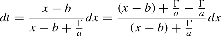
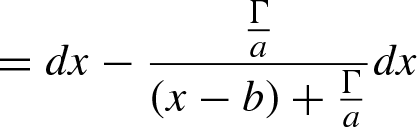
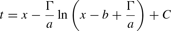
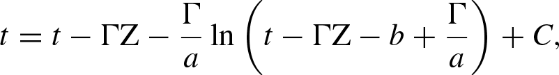
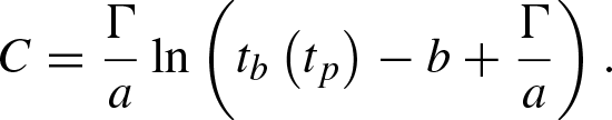
Therefore,

- Γ Z = \frac{Γ}{a} ln \frac{t - Γ Z - b + \frac{Γ}{a}}{t_{b} (t_{p}) - b + \frac{Γ}{a}},

as a result, we obtain

\frac{t - Γ Z - b + \frac{Γ}{a}}{t_{b} (t_{p}) - b + \frac{Γ}{a}} = \exp (- aZ)

(12)

This is the law of fluid flow temperature distribution along the length of the wells (when t = t_b) and the depth of the pump placement (when (t = t_p).

From Equation (10) we finally obtain

t_{cs} = Γ Z + b - \frac{Γ}{a} + (t_{b} - b + \frac{Γ}{a} \exp (- aZ))

(13)

where t_cs, t_b are the the current flow temperature in the CS as a function of distance and bottom hole temperature, respectively C_K, ⁰C.

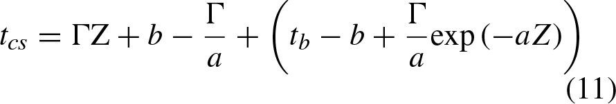
Thus, mathematical expression (11) describes the temperature distribution of the fluid flow along the length of the CS. This formula can also be used to determine the temperature of the upward flow along the length of the tubing, replacing the geometric gradient Γ with the temperature gradient in the fluid (at the distance of the depth of the pump placement under the dynamic liquid level in the CS) and gas (at the distance from the dynamic level to the mouth of the CS) layers of the CS $Γ_{∍}$ , i.e.

t_{t u b} = Γ_{∍} Z + b - \frac{Γ_{∍}}{a} + (t_{p} - b + \frac{Γ_{∍}}{a} exp (- a Z))

(14)

where t_tub is the current temperature of the fluid flow in the tubing, as the function of distance; t_p is the temperature at the pump inlet point, ⁰C.

The value of the heat transfer coefficient К, B_h/(m².⁰C) in the above formulas for determining the value of the coefficients a and b in OPW conditions can be determined from the following formula:

K = \frac{1}{\frac{1}{\propto_{1} D_{1}} + \frac{1}{2 λ} \ln \frac{D_{2}}{D_{1}} + \frac{1}{\propto_{2} D_{2}}}

(15)

where ∝₁ and ∝₂are the heat transfer coefficient from the fluid flow, the temperature of which is determined by formula (11), to the walls of the CS and from the CS wall to the rocks, W/(m². ⁰C), respectively; D₁ and D₂ are the inner and outer diameters of the CS, m; λ is the thermal conductivity coefficient, W/(m. ⁰C);

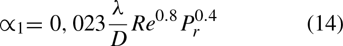
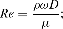
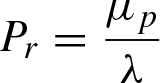
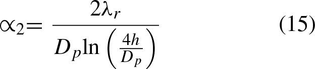
Similarly, we determine the value of the heat transfer coefficient K for the tubing, which differs in that the values of ∝₁, ∝ ₂, D₁, D₂, λ are determined in the upward fluid flow in the tubing; the values ∝₁ and ∝₂ can be determined from the following formulas:[12, 19]

\propto_{1} = 0, 023 \frac{λ}{D} {Re}^{0.8} P_{r}^{0.4}

(16)

Re = \frac{ρ ω D}{μ};

P_{r} = \frac{μ_{p}}{λ}

where Re, P_r are the Reynolds number and the Prandtl number, respectively; μ is the dynamic viscosity, mPa.s; c_P- is the specific heat capacity at constant pressure, kcal/(kg.⁰C)

\propto_{2} = \frac{2 λ_{r}}{D_{p} \ln (\frac{4 h}{D_{p}})}

(17)

where x is the distance from the outer surface of the lift pipe (the CS and the tubing), m; λ_r is the thermal conductivity of the rocks, W/(m. ⁰C); for different types of rocks, e.g., for quartz λ_q = 2.49; ∝_2q = 4.70; for clay, λ_c = 0.99, ∝_2c = 1.915 [19].

The schematic diagram of an oil production well (OPW) for which mathematical models (11)–(15) are proposed is shown in Fig. 2, in which the following designations have been adopted: 1 –rod string; 2 –sucker-rod pumping unit (SRPU); 3 –lift tubing; 4 –CS; 5 –annulus between the tubing and the CS, filled with gas-liquid mixture (GLM); 6 –distance from the bottomhole to SRPU intake; 7 –rocks; 8 –dynamic level (DL); 9 –distance from OPW bottomhole to DL.

Fig. 2

Schematic of an oil production well.

4 Conclusion

A systems analysis of the state of the art of heat transfer processes in the CS and the tubing of an oil-producing well has been carried out. Existing studies in mathematical modeling of the process of heat transfer from the upward fluid flow in the tubing to the annulus and in the CS to the rocks have been shown. Taking into account the geometric gradient of the rocks and heat transfer and thermal conductivity of the fluid flow in the tubing and fluid and gas in the annulus, new mathematical models have been proposed for determining the temperature distribution of the upward fluid flow along the length of the CS and the tubing, which allow to adequately estimate the heat transfer process in the tubing and the CS. Formulas have been proposed for estimating heat transfer from the fluid flow to the walls of the tubing and the CS (∝₁)and from the wall to the environment (∝₂).

References

Chekalyuk

E.B.

, Thermodynamics of an oil reservoir, M.: Nedra, 1965, 200 p.

Yu. Korobov,

, Mordvinov,

V.A.

, Temperature distribution along the wellbore of a production well, Moscow, Neftyanoye khozyaystvo, 2013, No 4, pp. 57–59.

Ye. Areshev,

, Plynin,

V.V.

Popov

O.K.

Shtyrlin,

V.F.

, Nature of anomalous data of thermohydrodynamic survey of oil wells Moscow, Neftyanoye khozyaystvo, 2000, No 3, pp. 41–47.

Guluyev

G.A.

Rzayev

Ab.G.

Rasulov

S.R.

, et al.Mathematical modeling of heat transfer process in an oil wellbore Moscow, Avtomatizatsiya, telemehanizatsiya i svyaz v neftyanoy promyshlennoy istorii, 2015, No 1, pp. 44–47.

Rzayev

Ab.G.

Guluyev

G.A.

, et al. The relationship between temperature differences at the wellhead and the production rate of oil wells Baku, Transactions of the Azerbaijan National Academy of Sciences, 2011, No 3, pp. 125–129.

Abbas Rzaev, Gambar Quliyev, , et al. Determining oil well debit using outlet temperature information processing, Proceeding of the sixth international conference on management science and engineering management, Springer Verlag, London, 2013, Vol. 1, Chap. 4, p. 55–64.

Rzaev

Ab.H.

Quliyev

G.A.

Pashayev

F.H.

, et al. Mathematical Models for determining the distribution of fluid flow temperature along the wellbore and horizontal pipeline, Mexatronika, Automatization, Control21(6) (2020), 337–347.

Mishchenko

I.T.

, Downhole oil production, M.: Neft i Gaz, 2003, 316 p.

Mordvinov

V.A.

Turbakov

M.S.

Yerofeyev

A.A.

, Method of evaluation of the beginning of intensive paraffinization of downhole equipment, Moscow, Neftyanoye khozyaystvo, 2010, No 7, pp. 112–115.

10.

Turbakov

M.S.

Yerofeyev

A.A.

, Results of the identification of the thermodynamic conditions for the formation of asphaltene-resin-paraffin deposits in the wells of a Siberian oil field Moscow, Neftyanoye khozyaystvo, 2010, No 11, pp. 106–107.

11.

Wong

, Handbook of essential formulae and data on heat transfer for engineers. Translated from English, -M.: Atomizdat, 1979, 216 p.

12.

Kasatkin

A.G.

, Main processes and machines of chemical engineering. –M.: –L. : Chemistry, 1960, 830 p.

13.

Leibenzon

L.S.

, Collection of works, Vol. 3, Oilfield mechanics, Moscow: Publishing House of the Academy of Sciences of the USSR, 1955, 520 p.

14.

Ivanova

L.V.

Burov

Ye.A.

Koshelev

V.N.

, Asphaltene-resin-paraffin deposits in the processes of production, transport and, storage, Electronic Scientific Journal Neftegazovoye Delo(1) (2011), 268–284.

15.

Persiyantsev

M.N.

, Oil production in complicated conditions, Moscow: Nedra-Biznestsentr LLC, 2000, 653 p.

16.

Tronov

V.P.

, Mechanism of resin-paraffin deposits formation and their control, M.: Nedra, 1970, 192 p.

17.

Klyumov

M.Sh.

Tronov

V.P.

Guskov

I.A.

Lapayev

A.A.

, Specifics of formation of asphaltene-resin-paraffin deposits at the late stage of oil field development, Neftyanoye Khozyaistvo, 2006, No 3, pp.48–49.

18.

Sorokin

S.A.

Khavkin

S.A.

, Specifics of physical and chemical mechanism of ARPD formation in wells, Burenie i Neft., 2007, No 10, pp. 30–31.

19.

Lutoshkin

G.S.

, Collection and treatment of oil, gas, and water for transportation. –M.: Nedra, 1972, 324 p.

20.

Shahnaz Shahbazova,

Julio Urenda,

Olga Kosheleva Vladik Kreinovich, , What Is the Uncertainty of the Result of Data Processing: Fuzzy Analogue of the Central Limit Theorem, International Journal of Acta Polytechnica Hungarica (2021), pp.69–76.

21.

Shahnaz Shahbazova

Dursun Ekmekci, , An input-weighted multi-objective evolutionary fuzzy classifier for alcohol classification, International Journal of Acta Polytechnica Hungarica (2021), 61–68.

22.

Shahnaz Shahbazova

Dursun Ekmekci, , Genetic algorithm-based adaptive weighted fuzzy logic control (AWFLC) for traction power control, Journal of Intelligent and Fuzzy Systems (2021), 6909–6916.