Multimodal prediction of breast cancer using radiogenomics and clinical trials with decision fusion

Abstract

Multimodal analysis focuses on the internal and external manifestations of cancer cells to provide physicians, oncologists and surgeons with timely information on personalized diagnosis and treatment for patients. Decision fusion in multimodal analysis reduces manual intervention, and improves classification accuracy facilitating doctors to make quick decisions. Genetic characteristics extracted on biopsies do not, however, provide details on adjacent cells. Images can only provide external observable details of cancer cells. While mammograms can detect breast cancer, region wise details can be obtained from ultrasound images. Hence, different types of imaging techniques are used. Features are extracted using the SelectKbest method in the Wisconsin Breast Cancer, Clinical and gene expression datasets. The features are extracted using Gray Level Co-occurrence Matrix from Histology, Mammogram and Sonogram images. For image datasets, the Convolution Neural Network (CNN) is used as a classifier. The combined features from clinical, gene expression and image datasets are used to train an Integrated Stacking Classifier. The integrated multimodal system’s effectiveness is shown by experimental findings.

Keywords

Convolution neural networks multimodal analysis gray level co-occurrence matrix histopathological mammogram sonogram and integrated stacking classifier

1 Introduction

Breast cancer is the most common cancer in women around the world. It is the second leading cause of death in women, but it is easily treatable if caught early. Extensive research has been devoted to detect breast cancer at an early stage. In the need for accurate and successful diagnosis within a limited period of time, the field of medical image processing acquires its significance. There is a need for automated processing because the manual process is tedious, time-consuming and inefficient for big data. For a medical professional to examine a single screening, it takes a considerable amount of time, effort and knowledge of earlier diagnosed cases.

Knowledge in the healthcare domain is acquired through experience and self-learning and is based on heuristics. Information explosion has exposed the potential of Machine Learning (ML) to aid in decision making for domain experts. It acts as a platform to collect information from heterogeneous resources and analyze the same to make suitable decisions. Machine learning is a computer program being developed to access the data and use it to learn by them. The primary objective is to allow computers to automatically learn without human interference or assistance, and to adapt actions accordingly, without being explicitly programmed.

Machine learning is mainly divided into two types; they are Supervised and Unsupervised learning. Most practical machine-learning employs supervised learning. X is the input variable and Y is the output variable consists of two variables in order to map the functions. The function (Y = f(X)) maps the function from input to the output variable, the supervised learning uses an algorithm for mapping the variables. For a particular input, the aim is to predict the output variable (Y). The method of learning from the training dataset is supervised learning. This learning has a teacher, supervises the learning process. The right answers are already known, the algorithm makes the repetitive predictions on the training data and the instructor corrects them. If the algorithm reaches the correct efficiency level, the level of learning will end. It is divided into Classification and Regression. In classification, A classification such as “disease” and “no disease” is the output variable. The output variable in a regression is a real value, such as weight.

There is no corresponding output variable in unsupervised learning since there is only one input data (X). Unsupervised learning does not have an instructor and there will not be correct answers. Algorithms are discovered to present the structure in the data. Unsupervised learning is categorised into two types - Clustering and Association. Clustering is grouping such as people in a group interested to buy a product. Association discovers rule that explains the patterns in the dataset, such as people that buy A will tend to buy B. The popularly used machine learning algorithms include:

1.1 Feature extraction algorithms

Feature selection is being introduced to decrease the irrelevant input variable so as to reduce the computational cost and also to improve the performance of the model. The methods of feature selection are roughly categorized into two techniques, Supervised and Unsupervised. The target variables are omitted in the Unsupervised Feature Selection Process, such as methods that neglect redundant variables using correlation.

The method of selection of supervised features uses the target variables, such as methods that exclude irrelevant features. The selection of the supervised function is split into wrapper, filter, and intrinsic methods. The wrapper method looks for well performing subset of features. The filter method chooses the subsets based on their relationship with the target and Intrinsic method uses algorithm that selects the automatic feature selection during training. The Dimensionality reduction projects the input data into the lower dimensional feature space.

In the Fig. 1, machine learning architecture is shown. Learning consists of training and testing phases. Training phase is to construct the model. During this phase, data is collected from the dataset, and the collected data is preprocessed. The feature extraction method is then implemented over the processed data. This is followed by feature selection phase that selects the relevant features. With the selected features, the model is constructed. During testing, relevant features are selected and the class is then identified using the classifier model.

Fig. 1

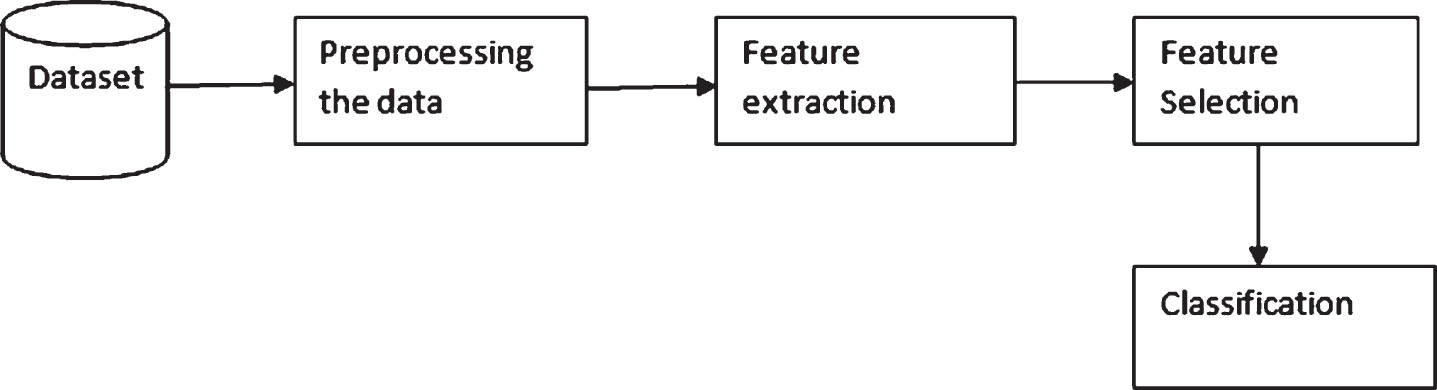
Basic architecture of machine learning system.

The process of machine learning includes parsing data, learning and decision making using suitable techniques represented as algorithms. Deep learning is a subgroup of Machine Learning. The paper proposes a convolution neural network and Integrated Stacking Classifier of Deep neural network. This speeds up the diagnosis, saves manual effort, and thereby helps in early detection of cancer and to improve the classification accuracy.

In the Fig. 2, CNN architecture comprises of various layers:

Fig. 2

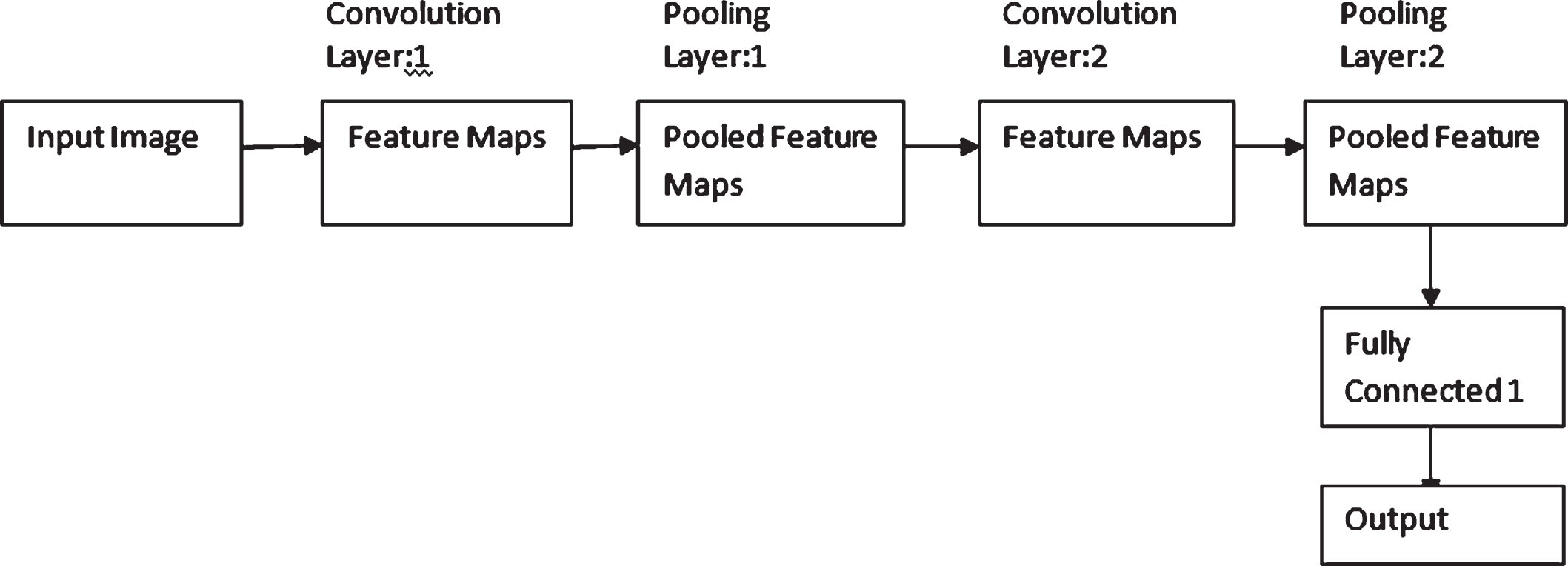
A CNN architecture.

CNN Layers:

Feature Maps: A CNN’s feature maps capture the result since the filters are placed in an input image. The layer performance is the list of functions at each layer. For a particular input picture the reason why a function map is visualized is to try to obtain some understanding of the CNN detects.

Pooling: It is a predefined that, in CNN architecture, the pooling layer is placed between successive convolutional layers. Its purpose is to slowly decrease the representation’s spatial scale. In essence, this decreases the number of network parameters and computation, and thus controls over-fitting. In each depth slice, the pooling layer often down-samples the volume spatially independently.

Fully Connected Layer: An input (a single vector) is received by Neural Networks and transformed into a hidden layer. Each secret layer consists of a collection of neurons in which each neuron in the previous layer is completely connected to all the neurons. Neurons operate entirely independently in a single layer and do not share any links. This layer is called as “output layer”.

Activation Function: Activation functions allow back-propagation as the gradients are provided along with the error to update the weights and biases. The activation function provides variety of nonlinearities for use in neural networks. These include smooth non-linearities (Sigmoid, tanh, relu, softplus and soft sign), (relu, relu6, crelu) and random regularization (dropout). All activation functions are applied component-wise, and produce the similar model as the input tensor.

Section 2 presents a review of literature on the state-of-art methods used for breast cancer prediction using various modes like mammograms, histology images and clinical datasets. Section 3 presents the proposed approach with a detailed description of various techniques used for feature selection and classification. Section 4 provides an experimental analysis on various unimodal approaches and the proposed multimodal approach with and without feature selection. Section 5 concludes on the results and analysis.

2 Related work

This study contains includes literature on feature selection, classification techniques used in gene expression, image, clinical data along with multimodal image analytics.

Qian Liu and Pingzhao Hu discussed about the a novel integrative framework for breast cancer radigenomics biomarker discovery. The author has used Bayesian tensor factorization (BTF) processing for the multi-genomic feature extraction. The datasets used for the analysis and the gene expression datasets are taken from The Cancer Genome Atlas (TCGA). The image datasets are collected from the The Cancer Imaging Archive platform. The design consists of Single radiogenomic stage and Multi radiogenomic stage. The Single radiogenomic stage is the base which has only gene expression as genomic data source. A Deep learning model 3DU-net was built, trained and validated to segment the tumor region from the three dimensional MRI image. After that the Deep Learning based radiomic features were extracted from the last hidden layer in the encoding phase. In the single radiogenomic stage, the paired data is used and lasso model are used to extract the features. Similarly the same process is carried out for the Unpaired data. In the multi radiogenomic stage, the Bayesian tensor Factorization is are used to extract the features in both paired and unpaired data. It is inferred that the Deep learning model gave a better performance. The leveraging strategy is used by the author [1].

Byung, Jingyu, Kangsan, Byung Hyun, Ilhan, Chang-Bae, Won Seok Song, Jae-Soo Koh and and Sang-Keun Woo discussed about the Radiogenomics affirmation for the prediction of Chemotherapy response for the pediatric patients. The prediction model is generated using the gene expression and image features. F-fluorodeoxyglucose positron emission tomography/computed tomography (F-FDG PET/CT) images are used for the prediction. Around 52 images are considered for the analysis. These images are fed into machine learning algorithm. Around 21 patients images were taken in order to develop the model. The accuracy measures such as Area Under Curve and Maximum image texture features are used. The random forest algorithm gave the highest accuracy. The chemotherapy response and metastasis test accuracy with image features gave an accuracy of 0.83 and 0.76 respectively. The highest test accuracy is around 0.85 and 0.89. The final conclusion is that the metastasis prediction accuracy is improved by 10% using the radiogenomics data [2].

Eun, Kwang, Bo and Kyu discussed about the machine learning methods to Radiogenomics of Breast Cancer. The machine learning approach is used to radiogenomics using low-dose perfusion computed tomography (CT) to predict prognostic biomarkers and molecular subtypes of invasive breast cancer.The study was done for the 241 patients who had invasive breast cancer. The 18 CT parameters are used for the analysis and five machine learning models are implemented. The machine learning models are SVM, Decision tree, Naïve Bayes, Random forest and artificial neural networks. Out of all these algorithms, the random forest model gave the better accuracy. The random forest had 13% highest accuracy and 0.17 higher AUC. The most important CT parameters in the random forest model are peak enhancement intensity, time to peak, blood volume permeability and perfusion of tumour [3].

David, Shanmugham and Amandeep discusses the classification methods for machine learning for the diagnosis of breast cancer. Linear Discriminant Analysis (LDA) has been used by the authors for feature selection. The classification algorithms used are Support Vector Machine, Artificial Neural Network and Naïve Bayes. Support Vector Machine outperformed with all the other classification methods. The authors concluded that the SVM-LDA is chosen as the best method, whereas NN-LDA takes longer computational time [4].

Siyabend and Mustafa used machine learning techniques for microarray breast cancer classification. Recursive feature Elimination (RFE) and Randomized logistic Regression (RLR) were used for feature selection. Support vector machine, KNN. Multilayer perceptron, decision tree, random forest, logistic regression, Adaboost, Gradient Boosting machines were used for classification. SVM classifier with RFE and RLR feature selection techniques provided better classification accuracy [5].

J.Arunadevi and Ganesh Moorthi discussed about the generalized linear method (GLM) and Random forest (RF) for feature selection. The Classification algorithms used includes K-Nearest Neighbour, Support vector machine and artificial neural networks. SVM classifier along with GLM feature selection outperformed compared other approaches [6].

Quang H.Nguyen Trang used PCA for feature selection. SVM, Random forest, KNN, Logistic regression, Ensemble voting, Adaboost and perceptron techniques were used for classification. Ensemble voting classifier, logistic regression, SVM and AdaBoost were observed to perform well compared to other models [7].

Sara, Peyman, Michal, Kevin and Ralph propose to identify histopathological biopsy images using the Deep Learning Network Ensemble method. The suggested model consists of three pre-trained CNNs, namely VGG19, MobileNet, and DenseNet. For the extraction and representation of characteristics, the ensemble model is used. The perceptron multi-layer is used as a classifier. The role extraction is performed using the transfer learning principle. Different combinations of hyperparameters including, optimizer, learning rate, weight initialization, batch size, dropout rate have been tried. The authors have used completely interconnected layers of the CNN architectures are combined to create the final feature vector [8].

Riu, Fei, Zihao, Lihua, Tong, Yudong, Xiaosong, Chunhou and Fa addressed the paper on the classification of breast cancer using hybrid profound neural networks. The image is divided into small patches, then using the CNN to identify each patch, and also its features are extracted, eventually combine the output of classification of these patches using majority vote. Additionally, Support Vector Machine is used for classification to render the output of the full histopathological images. The Multi-level feature extraction approach using CNN and RNN has been proposed. RNN is used to combine the patch feature to improve classification accuracy [9].

Phu, Tuan, Ngoc and Thuong addressed the multi-class classification of histology breast cancer images. The features from the image are in the form of vertical lines, horizontal lines and circles. The Convolutional Neural Networks were used for the image classification. The authors have used input layers, pooling layers, convolutional layers and Relu layers. The BreakHis dataset were used in this paper [10].

Yuqian Li, Junmin and Qisong addressed breast cancer classification based on deep learning using Multi Size and Discriminative Patches. The Feature extraction is done using two types of patches with different sizes from breast cancer histology images by using sliding window mechanism. This includes cell-level and tissue-level features. The Rest-Net 50 cluster is used to predict the tiny patches and to pick them with the likelihood of classification more than a threshold value. The extracted patches and selected patches from test image is fed into RestNet 50-512 and ResNet 50 clusters to get the group of dimensional features of 2048. The Three norm pooling method is used to calculate the last attribute of all the picture. The Support Vector Machine (SVM) is used as a final classification [11].

Anupama, Sowmya and Soman suggested using the capsule network with the histopathological images to identify breast cancer. The primary layer of the Capsule network is the Convolutional layer Capsule layer consists of 51 capsules. The authors proposed Capsule net architecture for the classification. The authors discussed that the stain normalization and patch extraction of the images and it is fed into the Capsule net architecture provides better accuracy [12].

Akshat has proposed Multimodal analysis on Clinical data, gene expression and image. The authors have used the Convolution Neural Network (CNN) for image classification. The clinical data and gene expression data are analysed with the help of machine learning classification algorithms K-Nearest neighbor Algorithm (KNN) and Support Vector Machine (SVM). The combined dataset of image, clinical data and gene expression are given as an input to the SVM. The Principal Component Analysis (PCA) is used to extract the features. SVM has given the best accuracy with all the three datasets and features [13]. The authors has used only one image dataset and the features are extracted and it is given as an input to the SVM.

In the proposed work, the multiple datasets such as Wisconsin Breast Cancer Dataset, Gene expression data [14], Clinical data and different image datasets (Histology, Mammogram and sonogram images) [15] are considered for the analysis. The features are extracted by using different feature selection methods from all the datasets and they are integrated. The combined model is implemented using the Integrated Stacking classifier which consists of five neural network models.

Anika and Olivier proposed deep learning with multimodal representation for the cancer prediction. The authors has used clinical, gene and WSI dataset for the prediction. The Unsupervised patient encodings are predictive and patients with similar characteristics tend to form a cluster. These feature representations act as an integrated multi-modal patient profile that can be used for classification. The authors has implemented CNN for unsupervised learning between clinical data, gene data and image dataset. The CNN is forced to develop the unique, consistent representation for an individual patient. The authors has used only one image dataset for the prediction and used CNN for the classification approach [14].

Literature review indicates the analysis of either one type of data set or multimodal fusion of image datasets. In the proposed approach, clinical, gene expression and different modes of image datasets is considered. Various The feature extraction approaches are then applied on the datasets. Finally, the combined model is implemented using the Integrated Stacking Classifier.

In the Table 1, Literature review indicates the analysis of either one type of data set or multimodal fusion of image datasets. In the proposed approach, clinical, gene expression and different modes of image datasets is considered. Various feature extraction approaches are then applied on the datasets and selected the best feature extraction method. Finally, the combined model is implemented using the Integrated Stacking Classifier.

Table 1
Literature survey on various machine learning algorithms and state of art approaches

S.No Paper Feature Selection Classification Advantages Disadvantages Dataset

1. A novel integrative computational framework for breast cancer radiogenomic biomarker discovery Deep learning and Bayesian tensor factorization Deep learning model Leveraging Strategy is used by the author for the first time in order to solve the unpaired data. One disadvantage of matrix deconvolution is that it cannot keep the inherent and complement information of different biological levels because matrix deconvolution method simply merges different molecular omics data matrix into a big data matrix without consider the interaction between them The datasets are The Cancer Genome Atlas (TCGA). The image datasets are collected from the The Cancer Imaging Archive platform

2 Preliminary Radiogenomic Evidence for the Prediction of Metastasis and Chemotherapy Response in Pediatric Patients with Osteosarcoma Using F-FDG PET/CT, EZRIN, and KI67 The image features are selected based on the AUC-Max value. Medcalc is used to determine the AUC Value of every image Random forest and gradient Boosting algorithms are used for the classification Out of all the machine learning algorithms, the Random forest gave the better accuracy. The radiogenomics technology along with the image features and gene expression certainly predict metastasis and Chemotherapy responses. With out the image feature and gene expression it is tough to predict the chemotheraphy and metastasis of the patient Real time dataset is used for the prediction

3 Machine Learning Approaches to Radiogenomics of Breast Cancer using Low-Dose Perfusion Computed Tomography: Predicting Prognostic Biomarkers and Molecular Subtypes The 18 CT parameters are considered for the analysis Support Vector Machine, Random forest, Decision tree, Artificial Neural Network and Naïve Bayes are used for the classofication. Machine learning method to radiogenomics using low dose perfusion breast CT is a useful invasive tool for predicting the biomarkers in invasive breast cancer Without the CT parameters the machine learning model will not provide better accuracy Real time dataset is used for analysis

4. Machine Learning classification techniques for breast cancer diagnosis In this paper, Linear Discriminant Analysis (LDA) is used for feature selection The classification algorithms used are: 1.Support vector machine 2.Artificial neural network 3.Naive Bayes Out of all the classifiers, the SVM outperforms of all the other classification algorithms. The hybrid approach SVM along with LDA gave better accuracy SVM-LDA is chosen as the best one. Whereas NN-LDA takes longer computational time. Wisconsin diagnostic breast cancer dataset is used in this paper.

5. Microarray breast cancer data classification using machine learning methods Recursive Feature Elimination (RFE) and Randomized logistic Regression (RLR) are used in this paper. The classification algorithms are: 1. Support Vector Machine. 2. KNN 3.Multi-layer perceptron 4. Decision tree 5.Random forest 6.Logistic regression 7.Adaboost 8.Gradient Boosting Machines The SVM classifier gave the best classification with both datasets after the feature selection methods. The accuracy level does not change by adding the neurons and layers. Without the feature selection, the accuracy level will not be able to improve. In this paper, two different datasets have been used. The first dataset has 133 samples with 1919 features. The second dataset has 97 samples with 24481 features.

6. Feature Selection Facilitated Classification For Breast Cancer Prediction Generalized Linear method (GLM) and Random forest The classification algorithm are: 1.K-Nearest neighbour 2.Neural networks 3.Support vector machine Out of all the classifiers, SVM with GLM feature selection have an accuracy of 91.3%. The authors has concluded that the SVM is the best classifier. The authors said that other types of feature selection and their strategies need to be concentrated along with other classifiers to increase the performance of the classification. The data reduction could also be used for the breast cancer classification “Breast cancer Coimbra”-donated by Patricio and it is available in the UCI repository

7. Breast cancer prediction using feature selection and Ensemble voting Principal component Analysis (PCA) is used. The classification algorithm used is: 1.K-Nearest Neighbour 2.SVM 3.Logistic regression 4.Stochastic gradient descent 5.Perceptron 6.Adaboost 7.XGBoost 8.Ensemble voting classification Out of all the 9 classifiers, the top 4 models are chosen based on the accuracy of about 98%, and the models are as follows: 1.Ensemble voting 2.Logistic regression 3.SVM tuning 4.AdaBoost Ensemble voting model classifiers can be used in other health care sectors. To reduce the human errors and false positive, Using this model, the other features could be used to improve specificity and accuracy. The dataset is used by the authors: Wisconsin breast cancer dataset from UCI repository

8. Classification of Histopathological Biopsy Images Using Ensemble of Deep Learning Networks -2019 ACM The model will learn general features from a source dataset that do not exist in the current dataset using a transfer learning approach. Transfer learning has many benefits, including accelerating network convergence, lowering computing capacity, and improving network efficiency. The three path ensemble architecture are used for classification: VGG19 MobileNetV2 and DenseNet201 are used for classification. The three path ensemble architecture is used in order to improve the classification accuracy. The InceptionV3, InceptionresNetV2, Xception, ResNet50, MobileNetV2 and DenseNet201, VGG19 and VGG16) with different combination of hyper parameters like optimizer, learning rate, weight initialization, batch size, dropout rate to obtain the best possible performance for breast cancer detection. Deep learning and blockchain technologies can be mixed. Stable data ownership control of electronic medical data or medical IoT devices is possible with blockchain. BreakHis is a dataset that contains 7909 H&E stained microscopic images obtained from 82 unidentified patients.

9. Breast cancer histopathological image classification using a hybrid deep neural network –2019 Elsevier For function extraction, the TensorFlow slim distribution’s pretrained Inception-V3 is used. The classification is done using a bidirectional long short-term memory network (BLSTM). LSTM has been extended.. The authors suggest a new hybrid model that incorporates both hybrid convolutional and recurrent deep neural networks. The use of the attention system in deep learning can be adapted, according to the authors. 3771 high-resolution (2048 * 1536 pixels) and annotated hematoxylin and eosin (H&E) stained breast pathological images make up the image dataset.

10. Multiclass Breast Cancer Classification Using Convolutional Neural Network –2019 IEEE The features extracted from the image are horizontal lines, vertical lines and circles The Convolutional Neural Network is used in this paper For the classification, the input layers, the convolutional layers, Relu layers and pooling layers are required. It’s a new challenge to classify eight subclasses of breast cancer in the BreakHis dataset. The accuracy can be improved by experimenting with various classification methods and optimising the parameters. The BreakHis dataset is used in this paper

11. Classification of Breast Cancer Histology Images Using Multi-Size and Discriminative Patches Based on Deep Learning The final features of images are extracted using CNN, Restnet50, and P-norm pooling. The authors has proposed image wise classification. The authors has discriminated 128 x128 pixel patches on cluster algorithm and CNN. SVM is used for final image classification. The lack of smaller patches with cell-level features makes it difficult to distinguish between normal, benign, and in situ carcinoma histology images. The dataset consists of high-resolution (2048 1536 pixels) and H&E stained breast cancer histology images from the bioimaging 2015 breast histology classification challenge.

12. Breast Cancer Classification using Capsule Network with Preprocessed Histology Images -2019 IEEE The primary layer of the capsule network is convolution layer, which is used to extract the feature of the histology image. Capsule layer is the next layer which consists of 51 capsules The authors has proposed the capsule net architecture for the classification The authors discussed that the stain normalization and patch extraction of the images and it is applied to capsule net architecture the accuracy level is performed. This method when it is automated, it can be used as a tool by the doctor, where the early prediction can be made. The dataset used for breast cancer classification is obtained from BACH 2018 grand challenge. The dataset consists of 285 histology stained images.

13. Cancer Prediction using Multimodel analysis The Contribution of the paper includes: 1.Principal Component Analysis (PCA) - for clinical and gene dataset. 2.Convolution Neural Network (CNN) –for image dataset The algorithms used are: 1.Support Vector Machine 2.K-Nearest Neighbour 3.Convolution Neural Networks 4.Logistic regression Multimodel analysis is time consuming because it is integrated and it works automatically. Multimodel not only reduces the time, it improves Overall accuracy. The ID and the columns were not suitable for all the images, so the authors has not considered all the images in the dataset, only sample images are used. The image dataset are taken from http://www.becominghuman.ai. The clinical and gene expression dataset are taken from http://www.dataworld.com

14. Deep Learning with Multimodal Representation for Pancancer Prognosis Prediction Feature selection is done using encoding methods and CNN. For classification CNN is used. The encoding is widely useful in number of context ranging from prediction to treatment recommendation In this paper only selected patches from WSI images are used. It is better to refine the layers of CNN for better accuracy. The dataset is taken from The Cancer Genome Atlas Program (TCGA)

S.No	Paper	Feature Selection	Classification	Advantages	Disadvantages	Dataset
1.	A novel integrative computational framework for breast cancer radiogenomic biomarker discovery	Deep learning and Bayesian tensor factorization	Deep learning model	Leveraging Strategy is used by the author for the first time in order to solve the unpaired data.	One disadvantage of matrix deconvolution is that it cannot keep the inherent and complement information of different biological levels because matrix deconvolution method simply merges different molecular omics data matrix into a big data matrix without consider the interaction between them	The datasets are The Cancer Genome Atlas (TCGA). The image datasets are collected from the The Cancer Imaging Archive platform
2	Preliminary Radiogenomic Evidence for the Prediction of Metastasis and Chemotherapy Response in Pediatric Patients with Osteosarcoma Using F-FDG PET/CT, EZRIN, and KI67	The image features are selected based on the AUC-Max value. Medcalc is used to determine the AUC Value of every image	Random forest and gradient Boosting algorithms are used for the classification	Out of all the machine learning algorithms, the Random forest gave the better accuracy. The radiogenomics technology along with the image features and gene expression certainly predict metastasis and Chemotherapy responses.	With out the image feature and gene expression it is tough to predict the chemotheraphy and metastasis of the patient	Real time dataset is used for the prediction
3	Machine Learning Approaches to Radiogenomics of Breast Cancer using Low-Dose Perfusion Computed Tomography: Predicting Prognostic Biomarkers and Molecular Subtypes	The 18 CT parameters are considered for the analysis	Support Vector Machine, Random forest, Decision tree, Artificial Neural Network and Naïve Bayes are used for the classofication.	Machine learning method to radiogenomics using low dose perfusion breast CT is a useful invasive tool for predicting the biomarkers in invasive breast cancer	Without the CT parameters the machine learning model will not provide better accuracy	Real time dataset is used for analysis
4.	Machine Learning classification techniques for breast cancer diagnosis	In this paper, Linear Discriminant Analysis (LDA) is used for feature selection	The classification algorithms used are: 1.Support vector machine 2.Artificial neural network 3.Naive Bayes	Out of all the classifiers, the SVM outperforms of all the other classification algorithms. The hybrid approach SVM along with LDA gave better accuracy	SVM-LDA is chosen as the best one. Whereas NN-LDA takes longer computational time.	Wisconsin diagnostic breast cancer dataset is used in this paper.
5.	Microarray breast cancer data classification using machine learning methods	Recursive Feature Elimination (RFE) and Randomized logistic Regression (RLR) are used in this paper.	The classification algorithms are: 1. Support Vector Machine. 2. KNN 3.Multi-layer perceptron 4. Decision tree 5.Random forest 6.Logistic regression 7.Adaboost 8.Gradient Boosting Machines	The SVM classifier gave the best classification with both datasets after the feature selection methods.	The accuracy level does not change by adding the neurons and layers. Without the feature selection, the accuracy level will not be able to improve.	In this paper, two different datasets have been used. The first dataset has 133 samples with 1919 features. The second dataset has 97 samples with 24481 features.
6.	Feature Selection Facilitated Classification For Breast Cancer Prediction	Generalized Linear method (GLM) and Random forest	The classification algorithm are: 1.K-Nearest neighbour 2.Neural networks 3.Support vector machine	Out of all the classifiers, SVM with GLM feature selection have an accuracy of 91.3%. The authors has concluded that the SVM is the best classifier.	The authors said that other types of feature selection and their strategies need to be concentrated along with other classifiers to increase the performance of the classification. The data reduction could also be used for the breast cancer classification	“Breast cancer Coimbra”-donated by Patricio and it is available in the UCI repository
7.	Breast cancer prediction using feature selection and Ensemble voting	Principal component Analysis (PCA) is used.	The classification algorithm used is: 1.K-Nearest Neighbour 2.SVM 3.Logistic regression 4.Stochastic gradient descent 5.Perceptron 6.Adaboost 7.XGBoost 8.Ensemble voting classification	Out of all the 9 classifiers, the top 4 models are chosen based on the accuracy of about 98%, and the models are as follows: 1.Ensemble voting 2.Logistic regression 3.SVM tuning 4.AdaBoost	Ensemble voting model classifiers can be used in other health care sectors. To reduce the human errors and false positive, Using this model, the other features could be used to improve specificity and accuracy.	The dataset is used by the authors: Wisconsin breast cancer dataset from UCI repository
8.	Classification of Histopathological Biopsy Images Using Ensemble of Deep Learning Networks -2019 ACM	The model will learn general features from a source dataset that do not exist in the current dataset using a transfer learning approach. Transfer learning has many benefits, including accelerating network convergence, lowering computing capacity, and improving network efficiency.	The three path ensemble architecture are used for classification: VGG19 MobileNetV2 and DenseNet201 are used for classification.	The three path ensemble architecture is used in order to improve the classification accuracy. The InceptionV3, InceptionresNetV2, Xception, ResNet50, MobileNetV2 and DenseNet201, VGG19 and VGG16) with different combination of hyper parameters like optimizer, learning rate, weight initialization, batch size, dropout rate to obtain the best possible performance for breast cancer detection.	Deep learning and blockchain technologies can be mixed. Stable data ownership control of electronic medical data or medical IoT devices is possible with blockchain.	BreakHis is a dataset that contains 7909 H&E stained microscopic images obtained from 82 unidentified patients.
9.	Breast cancer histopathological image classification using a hybrid deep neural network –2019 Elsevier	For function extraction, the TensorFlow slim distribution’s pretrained Inception-V3 is used.	The classification is done using a bidirectional long short-term memory network (BLSTM). LSTM has been extended..	The authors suggest a new hybrid model that incorporates both hybrid convolutional and recurrent deep neural networks.	The use of the attention system in deep learning can be adapted, according to the authors.	3771 high-resolution (2048 * 1536 pixels) and annotated hematoxylin and eosin (H&E) stained breast pathological images make up the image dataset.
10.	Multiclass Breast Cancer Classification Using Convolutional Neural Network –2019 IEEE	The features extracted from the image are horizontal lines, vertical lines and circles	The Convolutional Neural Network is used in this paper	For the classification, the input layers, the convolutional layers, Relu layers and pooling layers are required.	It’s a new challenge to classify eight subclasses of breast cancer in the BreakHis dataset. The accuracy can be improved by experimenting with various classification methods and optimising the parameters.	The BreakHis dataset is used in this paper
11.	Classification of Breast Cancer Histology Images Using Multi-Size and Discriminative Patches Based on Deep Learning	The final features of images are extracted using CNN, Restnet50, and P-norm pooling.	The authors has proposed image wise classification.	The authors has discriminated 128 x128 pixel patches on cluster algorithm and CNN. SVM is used for final image classification.	The lack of smaller patches with cell-level features makes it difficult to distinguish between normal, benign, and in situ carcinoma histology images.	The dataset consists of high-resolution (2048 1536 pixels) and H&E stained breast cancer histology images from the bioimaging 2015 breast histology classification challenge.
12.	Breast Cancer Classification using Capsule Network with Preprocessed Histology Images -2019 IEEE	The primary layer of the capsule network is convolution layer, which is used to extract the feature of the histology image. Capsule layer is the next layer which consists of 51 capsules	The authors has proposed the capsule net architecture for the classification	The authors discussed that the stain normalization and patch extraction of the images and it is applied to capsule net architecture the accuracy level is performed.	This method when it is automated, it can be used as a tool by the doctor, where the early prediction can be made.	The dataset used for breast cancer classification is obtained from BACH 2018 grand challenge. The dataset consists of 285 histology stained images.
13.	Cancer Prediction using Multimodel analysis	The Contribution of the paper includes: 1.Principal Component Analysis (PCA) - for clinical and gene dataset. 2.Convolution Neural Network (CNN) –for image dataset	The algorithms used are: 1.Support Vector Machine 2.K-Nearest Neighbour 3.Convolution Neural Networks 4.Logistic regression	Multimodel analysis is time consuming because it is integrated and it works automatically. Multimodel not only reduces the time, it improves Overall accuracy.	The ID and the columns were not suitable for all the images, so the authors has not considered all the images in the dataset, only sample images are used.	The image dataset are taken from http://www.becominghuman.ai. The clinical and gene expression dataset are taken from http://www.dataworld.com
14.	Deep Learning with Multimodal Representation for Pancancer Prognosis Prediction	Feature selection is done using encoding methods and CNN.	For classification CNN is used.	The encoding is widely useful in number of context ranging from prediction to treatment recommendation	In this paper only selected patches from WSI images are used. It is better to refine the layers of CNN for better accuracy.	The dataset is taken from The Cancer Genome Atlas Program (TCGA)

3 Proposed work

The design of the proposed system consists of various phases as given in this section:

3.1 A. Feature Selection Method:

Feature selection is the method of choosing the features manually or automatically, which contributes most of the predicted variable or output. The feature selection is used in order to improve the accuracy of the model. Having irrelevant features in the data will decrease the accuracy. The following feature selection approaches are used:

1) SelectKBest method: The SelectKbest feature selection method is one of the best selection method. It selects the top features depending the value specified for K. This approach is used to select features from Wisconsin Breast Cancer Dataset, Clinical dataset and Gene expression dataset.

Algorithm:

Step: 1 Import SelectKbest and chi2

Step: 2 Set the dataset location

Step: 3 Select the best features by passing the parameters score function as chi2 and k value. The user will specify the K value; the output will be generated as per the k value.

Step: 4 With the dataset location specified, it selects the best features

2) Principal Component Analysis: PCA is a statistical technique that reduces data dimension and allows us to understand, plot data of lesser size relative to the original data. As the name suggests, PCA allows one to measure the key data components. Main components are essentially linearly uncorrelated vectors with a variance in data. From the key components top p is chosen. This approach is used for selecting features from Wisconsin Breast Cancer Dataset, Clinical dataset and Gene expression dataset.

Table 2
Parameters of CNN

Layer # 1 2 3 4

Type conv pool conv pool

Channel 256 – 256 –

Filter size 3x3 – 3x3 –

Pooling size – 2x2 – 2x2

Activation ReLu – ReLu –

Layer #	1	2	3	4
Type	conv	pool	conv	pool
Channel	256	–	256	–
Filter size	3x3	–	3x3	–
Pooling size	–	2x2	–	2x2
Activation	ReLu	–	ReLu	–

Algorithm:

Step: 1 Standardize the range: Standardize the range of the continuous variables so that each one of them contributes equally to the analysis. This can be done by Z = Value-mean/ Standard deviation.

Step: 2 Covariance Matrix calculation:

In this step, to identify any relationships there between the input data. The covariance is in the form of pxp Symmetric matrix, where p is the number of dimensions.

Step:3 Compute the Eigen values and Eigen vectors of the Covariance Matrix to find the principal components. Eigen values and Eigen vectors are Linear algebra concepts. Principal components are new variables that are constructed as linear combinations or mixture of initial variables.

Step:4 Feature vector: Feature vector is a matrix that has as columns the eigen vectors of the components.

Step:5 Recast the data along with the Principal component axes.

3) Convolution Neural Network (CNN):

The CNN is used for the feature extraction. The image dataset is given as an input to the convolution neural networks. The features extracted by CNN are not visible to the user. Hence Gray Level Co-occurrence Matrix is used in this paper.

The details of the network are illustrated in the given table followed by its visual representation:

4) Autoencoders: An auto-encoder is type of a neural network consists of one hidden layer. The units in hidden layer is based on the level of compression required. Auto-encoders are used before convolution layer to optimize and preprocess image so that information which contains no significant weightage can be eliminated to help in computation complex processing.

5) Gray Level Co-occurrence Matrix:

Statistically, It is a texture analysis approach that takes into account the spatial relationship of the pixels in the matrix of co-occurrence, or GLCM at the gray point. The texture is characterized by the GLCM, based on how often in an image and in a specified spatial relationship pixel pairs with specific values appear. The features of GLCM are energy, entropy, dissimilarity, contrast and homogeneity. This document provides instructions for style and layout, information on installing the Word template and how to submit the final version. The instructions are designed for the preparation of a camera-ready and accepted paper in MS Word and should be read carefully.

3.2 B. Gray Level Co-occurrence Matrix features:

1) Energy: Energy’s Returns the number of GLCM square elements. Range = [0 1] for a recurring image, the energy is one. The alternative for the energy property is also known as Uniformity.

2) Entropy: It is a random variable, having its highest value when all of the elements of C are equal.

3) Homogeneity: Returns a value that calculates the proximity of element distribution in the GLCM to the diagonal of the GLCM. The value ranges from 0 and 1. For the diagonal GLCM, the Homogeneity is termed as 1.

4) Contrast: Returns the intensity contrast calculation over the entire picture between a pixel and its neighbor.

5) Dissimilarity: (Difference Average) The mean distribution of the image’s gray level differences is calculated. A larger value means a greater difference between adjacent voxels in intensity values. These extracted features are then used to train an integrated classifier.

The Convolution Neural Network (CNN), Autoencoder and Gray Level Co-occurrence Matrix (GLCM) are implemented over the image datasets. Initially the CNN and Autoencoder are implemented over the different image datasets and the features are not visible in both feature extraction methods. Whereas, the GLCM is designed in such way that the features are visible, Henceforth, in the proposed method, GLCM feature extraction method is used.

3.1 Integrated stacking classifier

The integrated stacking classifier is that the sub-networks can be integrated into a larger multi-headed neural network, which will then learn the best way to inculcate the forecasting of every input from the sub-model. The combined model will look like a single, larger unit. The advantage of the model is that submodel outputs are made directly accessible to the meta-learner. Further, the weights of the submodel can also be updated.

In the proposed methodology, multimodal analysis is performed. In this multimodal approach, different datasets are considered for the analysis. They are Wisconsin Breast Cancer Dataset, Clinical dataset, Gene expression dataset, and image datasets. In the image datasets, three different types of images are considered. They are Histopathological, Mammogram, and Sonogram images. For all the three image datasets, the Gray Level Co-occurrence Matrix feature extraction is implemented and seven attributes are taken from all the image datasets and converted into.CSV file. All three individual CSV files are integrated into one.CSV file.

The SelectKbest method is used for extracting the features. The K value will be given by the user. In the Wisconsin Cancer dataset, there were around 32 features. Different combinations of K values such as 5, 10, 15 and 20 are assigned.Out of these K values, K = 15 gave better result. For the final model 15 features are considered. For the Clinical and gene expression dataset, there were around 17 features. The K values such as 5 and 8 are given. Out of these K values, K = 8 gave better result. For the final model 8 features are considered.

The clinical data consists of 16 features and the SelectKbest feature extraction method is applied to the dataset. The Selectkbest method is used to extract the features based on the K value. Once after features are extracted, the classification algorithm such as KNN, SVM and Naïve Bayes are applied and accuracy is calculated. The accuracy is verified for the different combinations of K values. The gene expression dataset consists of 16 features and the SelectKbest is used for feature extraction. After extracting the features, the classification algorithms such as KNN, SVM and Naïve bayes are implemented and the accuracy is monitored. The Wisconsin Breast Cancer Dataset Consists of 32 attributes and the features are selected using the SelectKbest method. Once after the features are extracted, the classification algorithms like KNN, SVM and Naïve bayes are used to check for the accuracy. Once after extracting the features from the individual dataset, the extracted features are combined and the.CSV file is created. The combined final.Csv file is fed into the Integrated Stacking Classifier and the prediction value is obtained.

In the Fig. 3, the combined features are given as an input to the Integrated Stacking classifier. The integrated stacking classifier consists of five Neural Network models Models such as Keras Sequential Model, Keras Functional Models, Standard Network Models, Shared Layers Model and Multiple Input and Output Models. The integrated stacking classifier produces the classification accuracy based on the number of epochs, training and testing data. The main aim of the work is that to prove that the combined features implemented using Integrated Stacking classifier of deep neural network gives better accuracy compared to other models.

Fig. 3

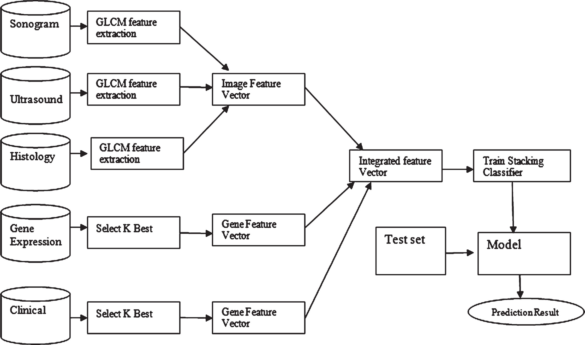
Proposed architecture.

4 Experimental results

The experiment is done by using Google Colab. The Google colab is an open source online tool provided by Google.

4.1 Datasets

1) Wisconsin Breast Cancer Dataset: The Dataset consists of 569 instances with 32 attributes; one attribute is the categorical attribute. There are no missing values in the dataset. Features are computed from the digital image of the breast mass.

2) Clinical Dataset and Gene Expression Dataset:

The breast cancer data was collected by the Netherlands Cancer Institute (NKI) [11]. It included clinical features but also gene expression levels; these represent how active genes and those that might contribute to cancer by being over-active or under-active. The dataset was taken from dataworld.com It included expression levels of the 1554 most variable genes and 17 clinical features and 17 gene expression features for 272 patients. Out of 17 clinical features, one feature is the categorical attribute called event death.

3) Image Dataset: The three different images are considered for the analysis, they are histology images taken from the BreakHis dataset [12] which consists of 2480 benign and 5429 malignant images. The mammogram images are taken from the Mammogram Image Analysis Society (MIAS, which has 322 images [15]. The sonogram images are collected from the women of ages between 25 and 75 years old. The data was collected in the year 2018. The numbers of female patients are 600. The dataset consists of 780 images with an average image size of 500x500 pixels [14]. The training and testing split considered for the Clinical and gene expression is dataset is 80% is for training and 20% is for testing. In case of the neural networks, the training set is considered as 80% and testing set is of 20%.

4.2 Feature extraction and selection

1) Features are extracted from image data set: Raw pixels of an image do not provide meaningful features to the classifier through which it may learn. An auto encoder can be used to extract the features. Gray Level Co-occurrence Matrix (GLCM) method is also used to extract the image datasets features and the csv file is generated for each image datasets. The GLCM extracts Mean, Entropy, Contrast, Homogenity, Dissimilar, Standard deviation and ASM are used for the analysis. The features extracted from each image are visible to the user. GLCM feature extraction is used and it extracts 7 features from the input images of all the different datasets. The performance of various feature extraction methods is shown in the figure.

In the graph, the x-axis represents the different datasets and y-axis represents the accuracy. From the Fig. 4, it is inferred that GLCM feature extraction gives better accuracy for both Mammogram which is 83% and for Ultrasound Images it is 85%, whereas for the Histology, the Autoencoder gave the better accuracy which provides 100%. Since GLCM gave better accuracy for both image dataset, the GLCM feature extraction method is used for all the images.

Fig. 4

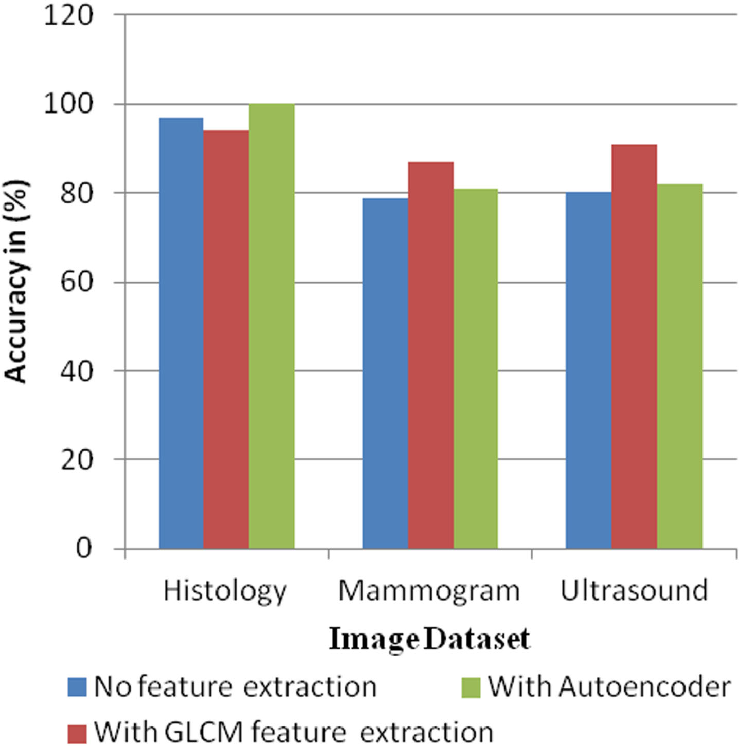
Accuracy comparison of feature selection approaches.

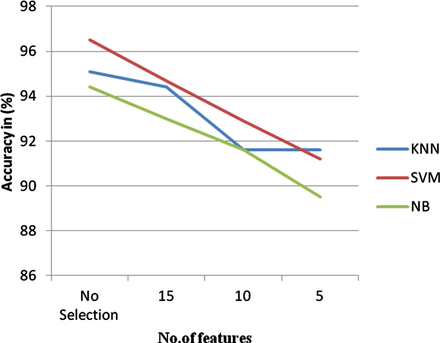
2) Feature selection for Wisconsin breast cancer dataset: SelectKbest and Principal Component Analysis methods are used for feature selection from clinical, geneexpression and Wisconsin datasets. Based on the Fig. 5, the 15 features were selected for Wisconsin dataset. The features are: area_worst, area_mean, area_se, perimeter_worst, perimeter_mean, perimeter_se, radius_worst, radius_mean, texture_worst, texture_mean, concavity_worst, radius_se, concavity_mean, compactness_worst, concave points_worst.

Fig. 5

SelectKbest feature selection in Wisconsin breast cancer dataset.

In the Fig. 5, the graph is represented between the features versus accuracy in percentage. It is inferred that the SVM gave better accuracy with no feature selection. The SelectKbest method is implemented with different feature sets. Out of 5, 10 and 15 features, with the 15 features, the classification accuracy improved compared to other set of features. With the increase in number of features, the classification accuracy started improving. Therefore the 15 features were considered as a final model. The three classification algorithms are implemented over the different sets of features, it is inferred that SVM gave better accuracy, when 15 features were selected. From the graph the SVM gives 97% accuracy with 15 features.

In the Fig. 6, the graph is shown between the features versus the accuracy in percentage. It is inferred that the SVM gave better accuracy with no features. The feature selection Principal Component Analysis is implemented with different feature sets. Out of 5, 10 and 15 features, with the 15 features, the classification accuracy is improved compared to other set of features. With the increase in number of features, the classification accuracy started improving. Therefore the 15 features were considered as a final model. The three classification algorithms are implemented over the different sets of features, it is inferred that SVM gave better accuracy, when 15 features were selected. The SVM obtains 97% of accuracy value for 15 features.

Fig. 6

Principal component analysis feature selection for Wisconsin breast cancer dataset.

Based on the comparison of SelectKbest method and PCA as shown in the Figs. 5 and 6, with the 5, 10, 15 and no features of Clinical dataset, the SelectKbest and PCA feature extraction algorithms are implemented, along with the algorithms KNN, SVM and Naïve Bayes, the SelectKbest gives 97% whereas the PCA gives 96.5% accuracy. Since the SelectKbest method provides better accuracy, the features are selected as per the SelectKbest method.

3) Feature selection in clinical dataset: SelectKBest and PCA techniques were tried for feature selection in clinical dataset using KNN, SVM and Naïve bayes Classifiers.

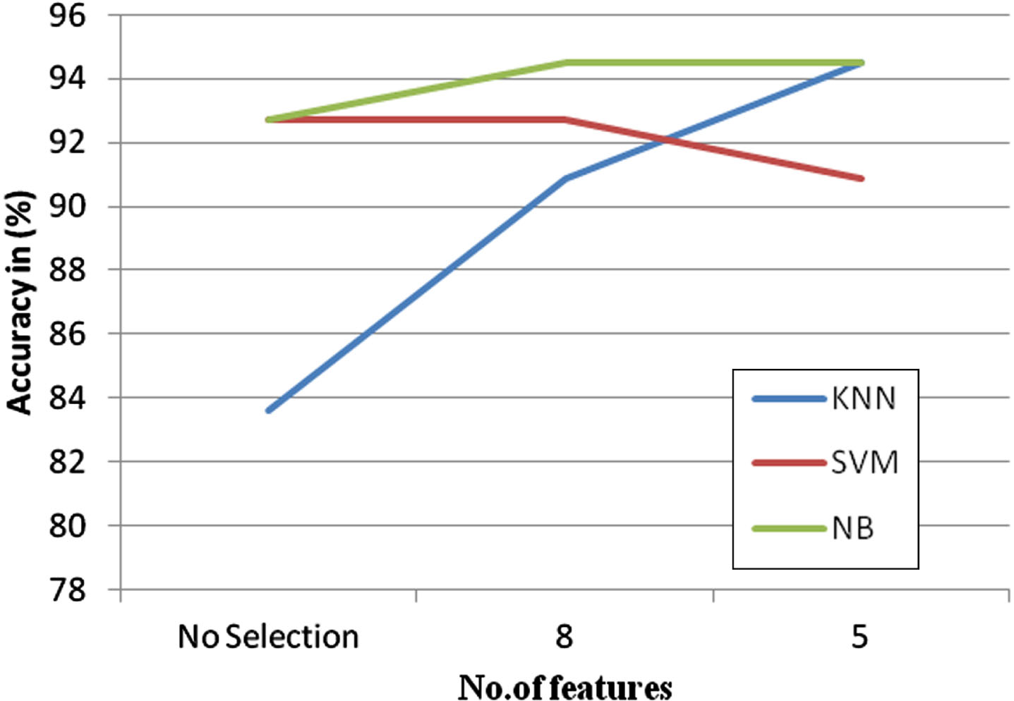
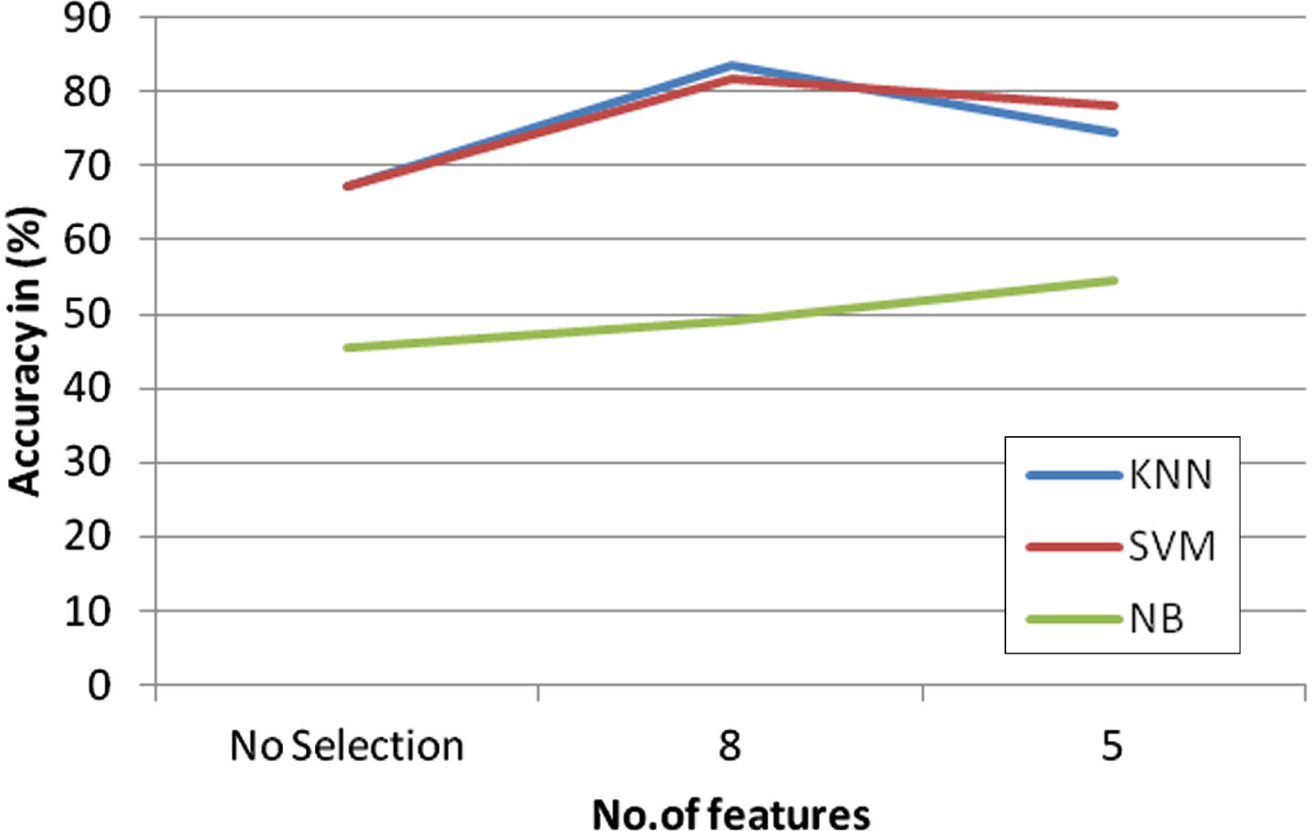
In the Fig. 7, the graph is represented between the features versus the accuracy. It is inferred that the SVM and Naïve Bayes gave better accuracy with no features. The feature selection SelectKbest method is implemented with different feature sets. Out of 5 and 8 features, with the 8 features, the classification accuracy is improved compared to other set of features. With the increase in number of features, the classification accuracy started improving. Therefore the 8 features were considered as a final model. The three classification algorithms are implemented over the different sets of features, it is inferred that Naïve Bayes gave better accuracy, when 8 features were selected.

Fig. 7

SelectKbest method in clinical dataset.

The features are:

Barcodes: barcode of the sample

Timerecurrence: Disease free interval in years between first date of the treatment and date of tumour recurrence.

Survival: Total Survival in years

Diam: Size of the tumour in mm

Grade: Grade of the tumour

Posnode: Number of cancer positive lymph nodes

Age: Age of the patient

Angioinv: presence of cancer cells in the blood vessel.

In the Fig. 8, the graph is drawn between the features and the accuracy in percentage. It is inferred that the SVM and Naïve bayes gave better accuracy with no features. The feature selection Principal Component Analysis is implemented with different feature sets. Out of 5 and 8 features, with the 8 features, the classification accuracy is improved compared to other set of features. With the increase in number of features, the classification accuracy started improving. Therefore the 8 features were considered as a final model. The three classification algorithms are implemented over the different sets of features, it is inferred that Naïve Bayes and SVM gave better accuracy when 8 features are selected.

Fig. 8

Principal component analysis feature selection for clinical dataset.

With the comparison of SelectKbest method and PCA as shown in the Figs. 7 and 8, with the 5,8 and no features of Clinical dataset, the SelectKbest and PCA feature extraction algorithms are implemented along with 3 algorithms, KNN, SVM and Naïve Bayes. It is inferred that with the 8 features along with Naïve Bayes and SVM gives 94% of accuracy, with PCA it gives on 92.5%, the SelectKbest method obtains better accuracy, hence,the features are selected as per the SelectKbest method.

4) Gene expression dataset: SelectKBest and PCA techniques were tried for feature selection in clinical dataset using KNN, SVM and Naïve bayes Classifiers.

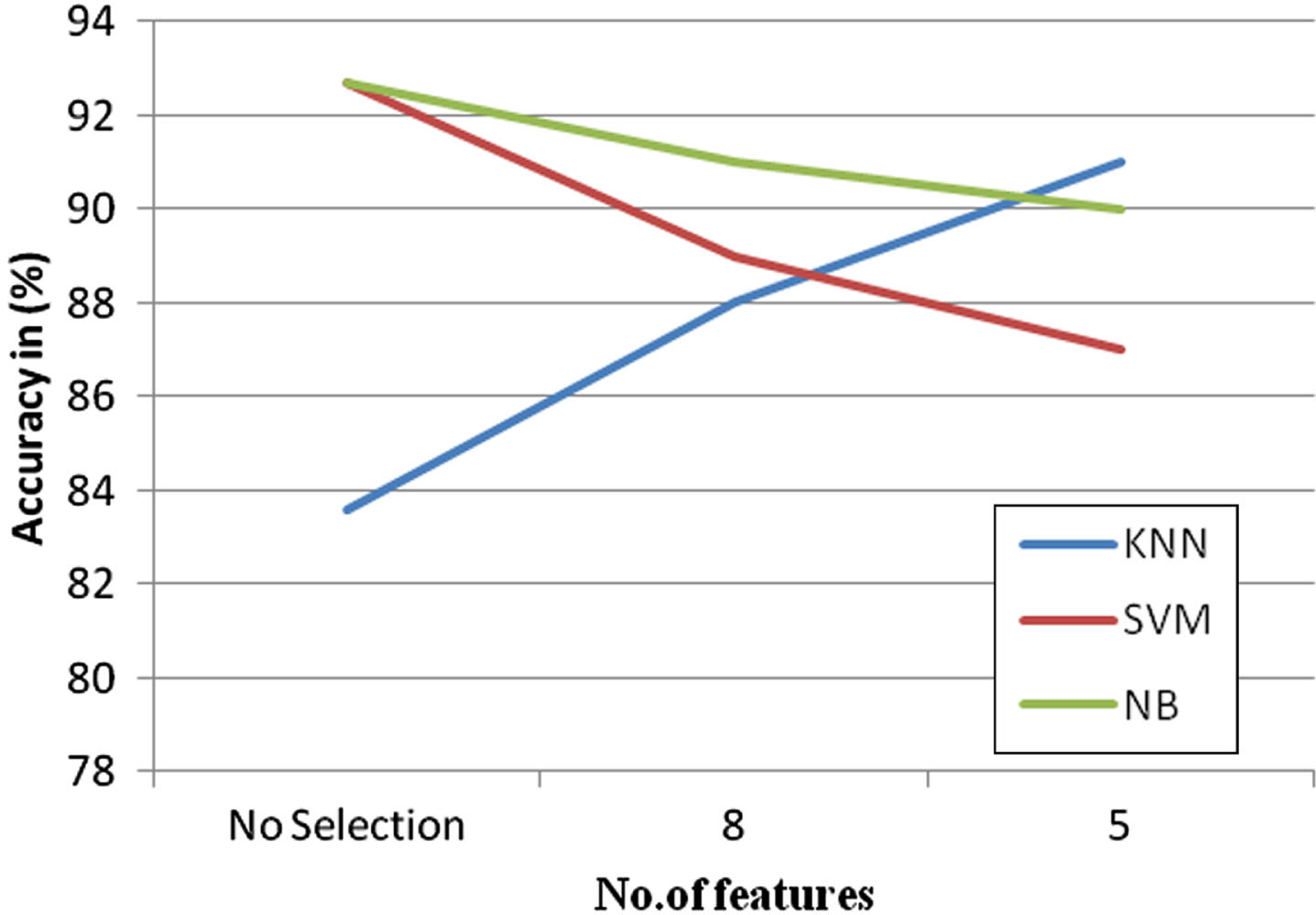
In the Fig. 9, the graph is represented with the features versus the accuracy in percentage, it is inferred that the SVM gave better accuracy with no features. The feature selection SelectKbest method is implemented with different feature sets. Out of 5 and 8 features, with the 8 features, the classification accuracy is improved compared to other set of features. With the increase in number of features, the classification accuracy started improving. Therefore the 8 features were considered as a final model. The three classification algorithms are implemented over the different sets of features, it is inferred that KNN gave better accuracy, when 8 features were selected.

The features are:

esr1 –Estrogen Receptor 1

Contig56678_rc –estrogen receptor

d25272 –Identifying early event of breast cancer

Al157502 - Widely found in different human tissues, the highest levels tend to express thymus and testis.

Contig44916_rc - The protein RCHY1 was located predominantly in the cytoplasm and membrane, and little in the malignant cell nucleus.

J00129- Gene category.

Contig20749_rc -: The RASSF tumor suppressor gene family (TSG) encodes Ras superfamily effector proteins that mediate some of the growth inhibitory functions of the Ras protein protein among its functions.

Contig37376_rc - The RBX1 gene is evolutionarily retained in each species, from plants to mammals with numerous family members.

Fig. 9

SelectKbest method in gene expression dataset.

In Fig. 10, the graph is represented between the features and the accuracy. It is inferred that the SVM better accuracy with no features. The feature selection Principal Component Analysis is implemented with different feature sets. Out of 5 and 8 features, with the 8 features, the classification accuracy is improved compared to other set of features. With the increase in number of features, the classification accuracy started improving. Therefore the 8 features were considered as a final model. The three classification algorithms are implemented over the different sets of features, it is inferred that KNN gave better accuracy when 8 features are selected.

Fig. 10

Principal component analysis feature selection for gene expression dataset.

With the comparison of SelectKbest method and PCA as shown in the Figs. 9 and 10, With 5,8 and no features of gene expression datas, the SelectKbest method and PCA feature extraction algorithms are implemented along with KNN, Naïve Bayes and SVM. With 8 features, SelectKbest method gives 85% of accuracy, whereas the PCA gives only 82%, hence the features are selected as per the SelectKbest method.

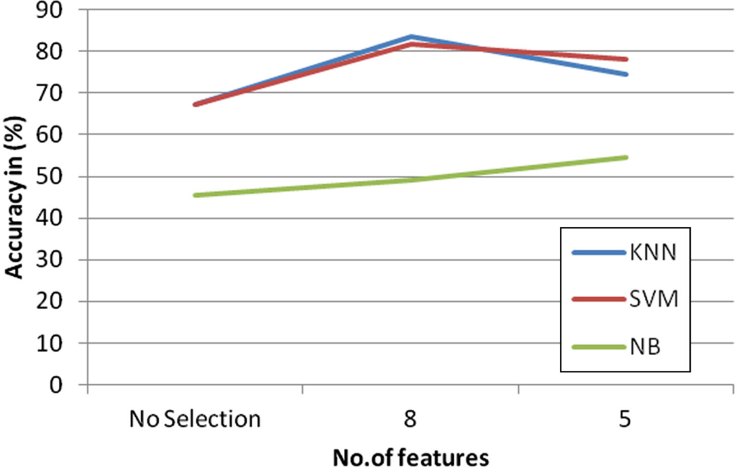
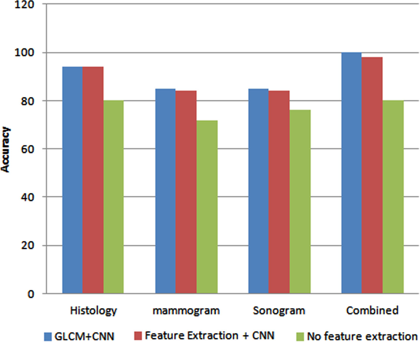
In the Fig. 11, the x-axis represents the different image datasets and the y-axis represents the accuracy obtained by using the feature extraction method. From the figure, the Histology, Mammogram, Sonogram and Combined (Histology+Mammogram+Sonogram) images are fed into the different feature extraction algorithms, Gray Level Co-occurrence matrix along with CNN, CNN and with no feature extraction, it is inferred that the Gray Level Co-occurrence matrix along with CNN gave better accuracy when compared to other methods in all the datasets. The number of training images taken for obtaining classification accuracy is 500, and the number of epochs for classification is 500.

Fig. 11

The accuracy of combined model using integrated stacking classifier is obtained.

The Histopathological image dataset are trained with 7200 images with 500 epochs gave 77% of accuracy. Around 322 Mammogram images are used for training and ran into 500 epochs gave an accuracy of 62%. Around 900 Ultrasound images are used for training with 500 epochs gave an accuracy of 74%. Similarly with 500 Histopathological image it gave an accuracy of 100%, with 500 images of mammogram images it gave around 78.6%, with 500 ultrasound image dataset the accuracy was around 80.4%.

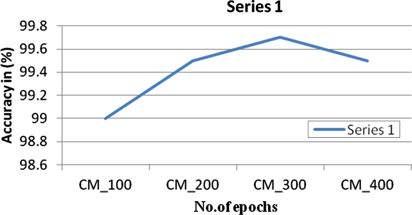
In the Fig. 12, the x-axis represents the number of epochs and the y-axis represents the accuracy in percentage. The Combined model consists of extracted features taken from Clinical dataset, gene expression dataset, Wisconsin breast cancer dataset and image dataset. All these Combined model is fed into the Stacking Classifier, compared to all other algorithms used, the Stacking classifier initially gave an accuracy of 99% with 100 epochs. As the epochs are increased the accuracy gradually increases as shown in the Fig. 12. This the maximum accuracy level attained. The Multimodal fed into the Integrated Stacking classifier outperforms with better accuracy compared to an individual model. Hence the Multimodal approach is an advantageous.

Fig. 12

Stacking classifier performance.

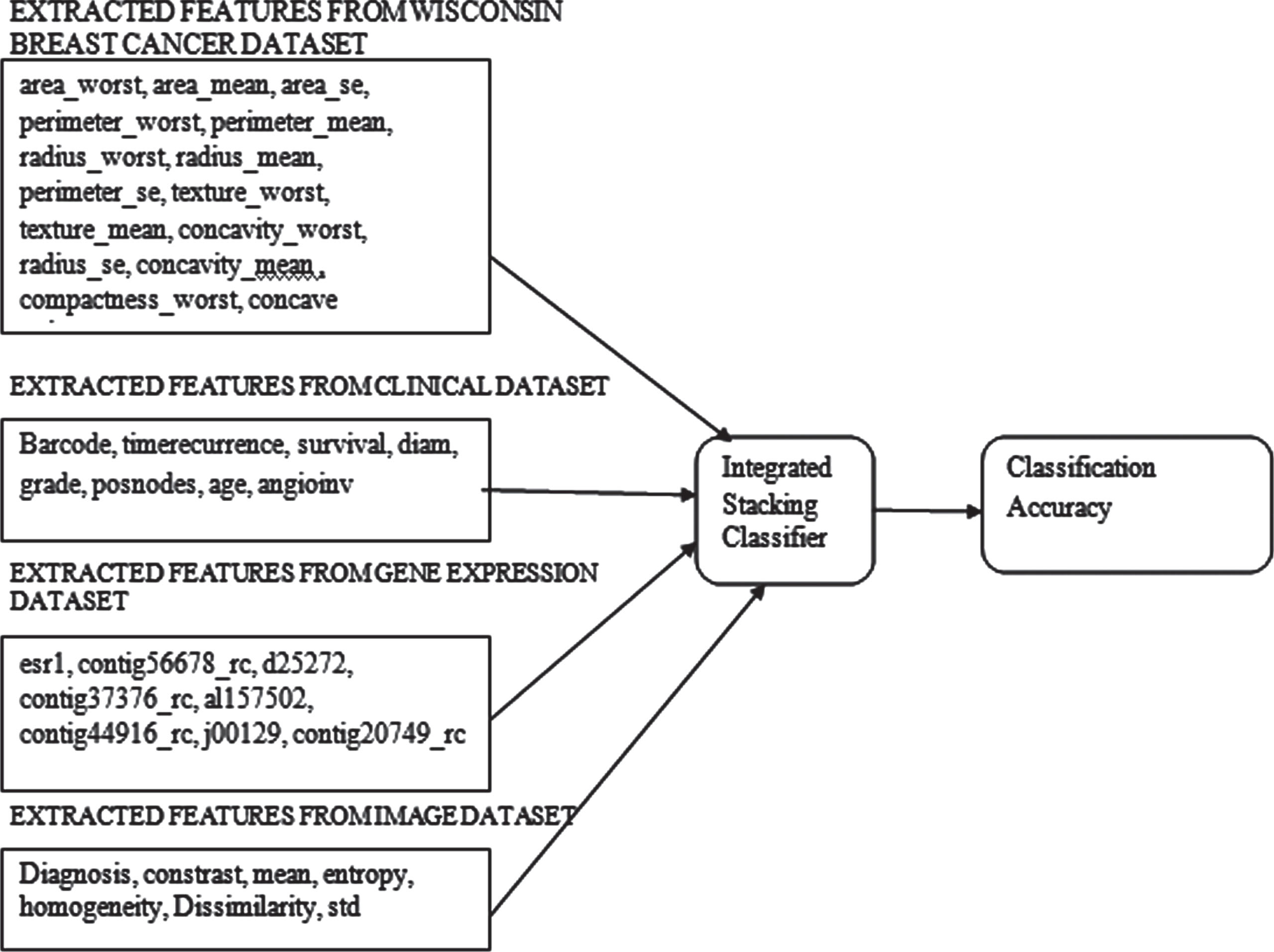
In the Fig. 13, the features extracted from all the three different datasets are combined together. All the features are combined and it is given as an input to the Integrated Stacking Classifier of deep neural networks. In the Integrated Stacking Classifier, the neural networks are the meta-learner. The sub-models are combined in a larger multi-headed neural network that learns to integrate predictions from all of the input sub-models. The stacking ensemble is treated as if it were one big model. The performance of the submodel is given to the meta-learner, which is a benefit of this classifier. Integrated Stacking Classifier outperforms compared to all other models.

Fig. 13

Extracted features from different datasets.

5 Conclusion

In this paper, the features are extracted from the different datasets by implementing the feature extraction methods, all the extracted features are combined together and fed as an input to the Integrated Stacking classifier. The developed model is applied for clinical data, images and gene expressions as a Multimodal approach. From our inferences, the multimodal classifier produces higher accuracy when compared to individual modes like gene expression or clinical or image data. The reason for giving us the highest accuracy is that the features are extracted and they are combined together into one single dataset, since relevant features are extracted from different datasets, it gave better accuracy.

6 Future work

The future work mainly based on the development of certain features which may or may not be incorporated in the existing system, they are remodeling the neural network to perform better. The other feature extraction method can also be incorporated.

References

Qian Lu , Pingzhao Hu A novel integrative computational framework for breast cancer radiogenomic biomarker discovery, Elsevier, Computational and Structural Biotechnology Journal (2022), 2484–2494.

Byung-Chul Kim , Jingyu Kim , Kangsan Kim , Byung Hyun Byun , Ilhan Lim , Chang-Bae Kong , Won Seok Song , Jae-Soo Koh , Sang-Keun Woo , Preliminary Radiogenomic Evidence for the Prediction of Metastasis and Chemotherapy Response in Pediatric Patients with Osteosarcoma Using 18F-FDG PET/CT, EZRIN, and KI67, MDPI, Cancers. https://doi.org/10.3390/cancers13112671 (2021), 1–11.

Akshat Katiyar , , Cancer prediction using multimodel analysis, International Journal of Engineering Research & Technology (IJERT)ISSN: 2278-0181 9(02) (2020), 172–175.

Eun Kyung Park , Kwang , Bo Kyoung , Kyu Ran , Machine learning approaches to radiogenomics of breast cancer using low-dose perfusion computed tomography: predicting prognostic biomarkers and molecular subtypes, Scientific Reports, Springer (2019), 1–11.

David Omondiagbe

, Machine learning classification techniques for breast cancer diagnosis, IOP Conference series: Materials Science and Engineering (2019), 1–16.

Dr.Arunadevi

, Ganeshmoorthi

Feature selection facilitated classification for breast cancer prediction, IEEE, International Conference on Computing Methodologies and Communication (ICCMC 2019) (2019), 560–563.

Quang , Trang , Yijing , Sin , Kelly , Wei , et al. Breast cancer prediction using feature selection and Ensemble voting, IEEE, International Conference on System Science and Engineering (ICCSE) (2019), 250–254.

Sara , Peyman , Michal , Kevin , Ralph , Classification of histopathological biopsy images using ensemble of deep learning networks, ACM, ISBN 978-1-4503-6317-4/19/07, 2019.

Rui , Fei , Zihao , Lihua , Tong , Yudong , Xiaosong , Chunhou , Fa , Breast cancer histopathological image classification using a hybrid deep neural network, Elsevier, Methods (2019), 1–9.

10.

Phu , Tuan , Ngoc , Thuong , Multiclass Breast Cancer Classification Using Convolutional Neural Network, IEEE (2019), 130–134.

11.

Yuqian , Junmin , Qisong , Classification of breast cancer histology images using multi-size and discriminative patches based on deep learning, IEEE Special Section On Deep Learning For Computer-Aided Medical Diagnosis (2019), 21400–21408.

12.

Anupama , Sowmya , Soman , Breast cancer classification using capsule network with preprocessed histology images, IEEE, International Conference on Communication and Signal Processing (2019), 143–147.

13.

Anika , Olivior , Deep Learning with Multimodal Representation for Pancancer Prognosis Prediction. BioRxiv (2019), 1–15.

14.

Siyabend , Mustafa , Microarray Breast cancer data classification using machine learning methods, IEEE (2018), 1–3.

15.

https://data.world/deviramanan2016/nki-breast-cancer-data-Clinicalandgeneexpressiondataset>.

16.

Center for Diseases Control and Prevention. https://www.cdc.gov/cancer/breast/basic_info/index.html.

17.

Histopathological images http://www.kaggle.com.

18.

Ultrasound images http://www.groundai.com.

19.

Mammogram images http://www.mammoimage.org.