Accelerating trail navigation for unmanned aerial vehicle: A denoising deep-net with 3D-NLGL

Abstract

Waypoints have enhanced the prospect of fully autonomous drone applications. However, Geographical Position System (GPS) spoofing and signal interferences are key issues in waypoint-based drone applications. Also, conceptual waypoint-based drone applications require accurate awareness of waypoints based on environmental cues and integration of additional sensing modalities. Additional sensor modalities may overwhelm drones’ processing resources, reducing operational time. This study proposes W-MobileNet, a denoising model for autonomous trajectory trail navigation based on precision control of a path planner, denoising capabilities of Weiner filters, and perceptual knowledge of convolutional neural networks. Creatively integrating the modules of W-MobileNet results in an intuitive drone navigation controller characterized by position, orientation, and speed estimation. Further, a generic loss function that significantly aids models to converge faster during training is proposed based on adaptive weights. An extensive evaluation of a simulated and real-world experiment shows that W-MobileNet is more favorable in precision and robustness than contemporary state-of-the-art models. W-MobileNet has the potential to become one of the standards for autonomous drone applications.

Keywords

Navigation waypoint drone unmanned aerial vehicle autonomous deep convolutional neural network

1 Introduction

Over a decade now, the robotics field, which encompasses Unmanned Aerial Vehicles herein UAV, has drastically transformed the industrial world in diverse tasks. The standard UAV on the market is usually equipped with single or multiple cameras, and its capability of flying, which gives it a broader view of terrains, is an advantage. As it stands now, UAVs are being utilized in fields such as search and rescue missions, aerial surveillance, agriculture technology, industrial inspection, military applications, package delivery, and many more [1]. UAVs can operate in indoor and outdoor environments, and with regards to control; it can be either a human-based or autonomous-based piloting. Due to the projected potential, much attention has been channeled to the automation aspect of UAV navigation. The continued development of deep learning is out-smarting human intelligence gradually in peculiar tasks, and it is only a matter of time before deep learning-based systems perform better than humans in unmanned systems navigation.

The desire to attain this uncensored achievement in UAV navigation has called for enormous research into autonomous UAV navigation, which dwells on sensors, knowledge-based models, and navigation algorithms (e.g., state-of-the-art path planners). Most outdoor UAV navigation methods in obstacle-free or obstacle-populated environments rely mostly on GPS, which has proven to some extent feasible, but not entirely desirable as the threats to GPS systems such as GPS spoofing is a continuous challenge. Besides, there are GPS non-functional zones, both outdoor and, to a large extent, indoor environments. Also, GPS is receptive to strong signal interferences when it encounters signals such as radio emissions in nearby bands and signals from jammers. Unstructured features within the environment usually challenge other UAV navigational methods based on conceptual waypoints which dwell on cues. Furthermore, in vision-based navigation, motion blur, aliasing, and other elements considered as noise can negatively influence the navigation of the UAV.

This study presents an attempt toward autonomous UAV navigation from the perspective of vision-based utilizing conceptual waypoints as a guide. For brevity, the contributions of the paper ensue as:

A framework, W-MobileNet that constitutes an adapted MobileNet [2], a variant Weiner filter [3] as a denoiser, and a variant path planner, the three-dimensional Non-Linear Guidance Law (3D-NLGL) [4] is proposed as a UAV navigational controller.

A novel loss function characterized by adaptive weights that facilitates faster model convergence during training is proposed.

Lastly, a simulated and real-world experiment is conducted with comprehensive comparisons with some state-of-the-art navigational controllers to ascertain the practicability of the proposed navigational controller. Experimental results indicate that W-MobileNet offers intuitive and precise navigation for the UAV.

The paper’s organization ensues as follows: Section 2 entails prior research conducted within the scope of UAV navigation, followed by Section 3, the methodology. In Section 4, we delineate the setup and the experiment conducted with concluding experimental results and analysis. The conclusion drawn on the work and feasible future works is given in Section 5.

2 Related works

Most of the existing UAV navigation works are categorized into two based on the operational environment, either obstacle-populated or obstacle-free. Within the operating environment, the navigation type is either waypoint navigation (i.e., following a predefined trail based on beacons or imaginary reference points) or path planning (i.e., exploratory navigation) [5]. The mechanism within the types of navigation usually is either map-aided, which dwells on proximity sensors for constructing maps of the environment, or a vision-based which does not use built maps.

2.1 Map-aided autonomous navigation

Reiterated literature based on map-aided navigation includes but is not limited to Simultaneous Localization and Mapping (SLAM) [6], Parallel Tracking and Mapping (PTAM) [7], and Structure from Motion (SfM) [8]. The methods mentioned above primarily utilize data readings from sensors (e.g., infrared, ultrasonic, and optical flow) in constructing a map. SLAM and PTAM build a 3D model/map of the environment based on the information from the sensors to aid a UAV during navigation. Light Detection and Ranging (LIDAR) and Sound Navigation and Ranging (SONAR) are utilized in obstacle-populated environments. Even though some of the methods above worked, the number of computing resources needed to build a 3D map may overwhelm the computing resources of a UAV. An optimal path for UAV localization based on the Kalman filter and data generated by an ultrasonic sensor attached to a UAV was proposed [9]. The authors estimated observation density which played a crucial role in their navigation based on a predefined constructed terrain map. Their aim was the altitude, collision avoidance, stability, and anti-drift control. In the retrospective findings of the authors, it was apparent the computational complexity and cost were high due to the number of heavyweight sensors attached to the UAV. As detailed in their work, three accelerometers and gyroscopes, four infrared sensors, an ultrasonic sensor, one high-speed motor, and a flight computer were used. Cruz et al. capitalized on the capabilities of proximity sensors to sense obstacles within an environment and constructed detectable obstacles on a 3D map to aid a UAV during navigation [10]. Other works in the space of 3D map construction for UAV navigation that utilizes LIDAR are that of Stubblebine et al., [9], Bachrach et al., [11], Vandapel et al., [12], Bry et al., [13], and Bachrach et al., [14]. Although the reconstruction of a map to aid the UAV in navigating is feasible, especially in obstacle-populated environments, it comes at the cost of extra usage of sensing modalities susceptible to calibration errors and high computational complexity. Again, methods based on reconstructing maps of an environment with fewer environmental features are prone to failure.

2.2 Vision-based autonomous navigation

From the viewpoint of vision-based navigation, a UAV navigated in an obstacle environment based on Reinforcement Learning (RL) and model predictive control [15]. A similar study used RL to guide a UAV to navigate an indoor environment [16]. Again, an RL and shooter model was adopted as a UAV navigation controller [17]. An exploit of [17] is that of Chao et al., [18] that utilized a model-free RL technique and not the standard Deep Neural Networks (DNNs) that were adopted in [19]. Although the RL approach toward autonomous UAV navigation eliminates the task of data labeling, its drawback is the overloaded states which can lead to diminishing results. In reality, using the RL method can be costly since its learning process is based on feedback from previous predictions (correct or wrong). Usually, wrong predictions lead to the crushing of the UAV hence wearing and tearing out. Reference [20] estimated the positions and orientations based on a computational efficient Convolutional Neural Network (CNN) that utilized transfer learning for UAV navigation. Despite the advantage of transfer learning in the authors’ proposition, their method exhibited large baselines, which can cause scale-invariant feature transform localizers to fail drastically. Again, the transfer of knowledge from one domain may not generalize to other disciplines with varying features in data (e.g., initializing a DCNN being trained to learn geometric features with ImageNet weights). A YOLO-based DCNN was used to process a video feed of a micro aerial vehicle to trail predefined paths [21]. Although the resulting section of the authors’ work indicated their method’s success, the learned policy’s generalization capabilities to an unseen environment were not established. Further, an anchor-based YOLO version was used, reducing inference speed and accuracy compared to anchor-free object detectors. An optimized DCNN compatible with varying image resolutions was proposed to aid a UAV in following a trail in an unstructured environment [22]. The authors acknowledged the limitation of generalization when their optimized DCNN was trained using low-to-high resolution images. Further, the proposition in the paper restricts the UAV to move in directions forward, back, left, and right only with a fixed altitude and speed.

Based on imitation learning, a Recurrent Neural Network (RNN) was trained end-to-end together with a Long-short-term-memory (LSTM) network to guide a UAV to navigate through a room [23]. The authors assert that a pre-trained network requires little training data and also serves as a reasonable basis for training new models hence lots of time is saved during training. Moreover, they argue that incorporating a limited time window in LSTM during training yields better results than training with previous images. Although the limited time window eliminates the correlation problem, it also leads to the problem of higher variances and computational complexity, which slows down the training process and reduces inference speed. A DCNN was trained as a supervised image classifier to guide a UAV to navigate a hiker’s trail [24]. The presented approach is limited to discrete orientation and positions, thus a limitation in the movement of the UAV. A two-class multilayer perceptron was proposed as a tracker and detector, which used mapped images from the front camera of a UAV for navigation during the inspection of aerial power lines [25]. The network was trained to classify background from objects within the environment to aid the UAV in navigating the inspected power line. Since the approach depends on extracting background information for motion estimation, it is challenging in environments with little background information.

Contrary to the numerous deep learning approaches used in UAV navigation, the proposed method in this study aims to control precision and eliminate additional sensing modalities for autonomous UAV navigation. The W-MobileNet framework sequentially is characterized by a denoiser for image restoration, a lightweight DCNN model for feature extraction and inference making, and a path-planner to streamline navigational commands. Next, the methodology section elaborates on the proposed method.

3 Methodology

3.1 Data

The Microsoft AirSim simulator [26] built on top of Unreal Engine, which provides a realistic synthetic environment, is used. The environment is set in the Landscape Mountains, characterized by snowy mountains, lakes, forests, and rocky lands. A Pixhawk-4 (PX4), which supports Software in The Loop (SITL), is used together with the Cygwin toolchain to manually fly the quadrotor (UAV) in the virtual environment to collect data (see Fig. 1). The manual flight covers 50 predefined waypoints over a distance of 750 meters, serving as the reference trajectory. Each waypoint has a gateway inspired by the AirSim drone racing lab [27]. The gateways serve two purposes: (i) as an evaluation metric; thus, to check if the UAV successfully passes through the gateway, and (ii) to aid visually the turn anticipation of the UAV, which helps in the tangential interception of a segment part of the reference trajectory. A total of 61,274 frames were collected together with flight telemetry and reposited at [28]. Data augmentation is carried out on 20% of the total frames to add slight variance to the data. The details of the data are tabulated in Table 1.

Fig. 1

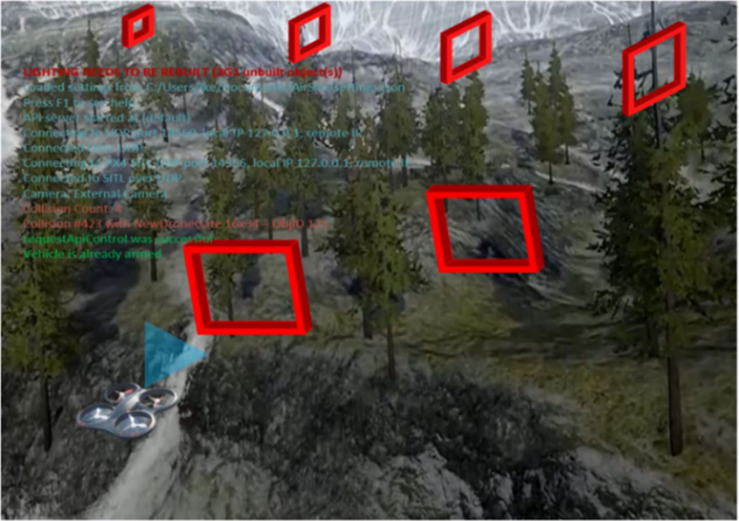
Illustration of manual flight through waypoints/gateways in the Landscape Mountain environment via Microsoft Airsim Simulator. The blue triangle indicates the Field of View (FOV) of the UAV.

Table 1

Summary of collected synthetic data

Synthetic environment	No. of frames	Augmented frames	Waypoints/Gateways	Distance
Landscape mountains	61,274	12,256	50	750m

3.2 Adaptive weiner filters

Within the RGB color space scheme (channels), pixels within each channel are subject to some perturbation (i.e., an adversarial attack that in the context of UAV navigation emanates as a result of the swift movement of the UAV collecting imagery data in an environment). An adversarial attack is a variety of noise (e.g., additive, Gaussian, and Poisson noises, respectively) that interferes with information within an image. A classical approach in handling adversarial attacks is using Weiner filters which find a trade-off between noise smoothing and inverse filtering by removing the noise and inverting the blurring effect based on mean square error. The Weiner filter in the frequency domain is given as: $G (f) = \frac{H^{*} (f) S (f)}{{| H (f) |}^{2} S (f) + N (f)}$ (1) where G (f) and H (f) are Fourier transforms, and the superscript * is a conjugate complex of the filter. Parameter S (f) denotes the mean power spectral density of some original signal x (t) . N (f) is the mean power spectral density of some noise n (t) which can be replaced with an experimental constant K . Despite the success of classical Weiner filters and some other restoration filters, such as inverse and pseudo-inverse filters, they are not adaptive. Further, they fail on spatially varying blur points. However, the adaptive Weiner filters possess adjustable hyperparameters which adjust to noise whose power spectrum alternates with time, hence feasible in mitigating variant adversarial attacks. Secondly, the adapted DCNN MobileNet is not explicitly optimized for image restoration such as the Generative Adversarial Networks; hence the adaptive Weiner filter [29] is utilized for image restoration. Further, since the blurring kernel is known in adaptive Weiner filters, it is advantageous compared to some DCNN pipelines that have to learn the blurring kernel before image restoration. Given an image that is corrupted (affected by an adversarial attack), the problem is formulated as: $y (i, j) = x (i, j) + n (i, j)$ (2) where y (i, j) represents the noisy measurement, x (i, j) is the image without noise, and n (i, j) is additive Gaussian noise. To get the linear estimate $\hat{x} (i, j)$ of the noisy-free image x (i, j), y (i, j) has to be denoised using the mean squared error (MSE) given as: $MSE (\hat{x}) = \frac{1}{N} \sum_{i, j = 1}^{N} {(\hat{x} (i, j) - x (i, j))}^{2}$ (3) where N is the number of entities within x (i, j). The adaptive Weiner filter is fused as a module in the W-MobileNet framework described in Section 3.3. Figure 2 shows the introduction of adversarial attacks on randomly selected frames (images) that have been denoised using adaptive Weiner filters. The reason for introducing the adversarial attack was the difficulty in choosing specific noisy frames out of the 61, 274 frames.

Fig. 2

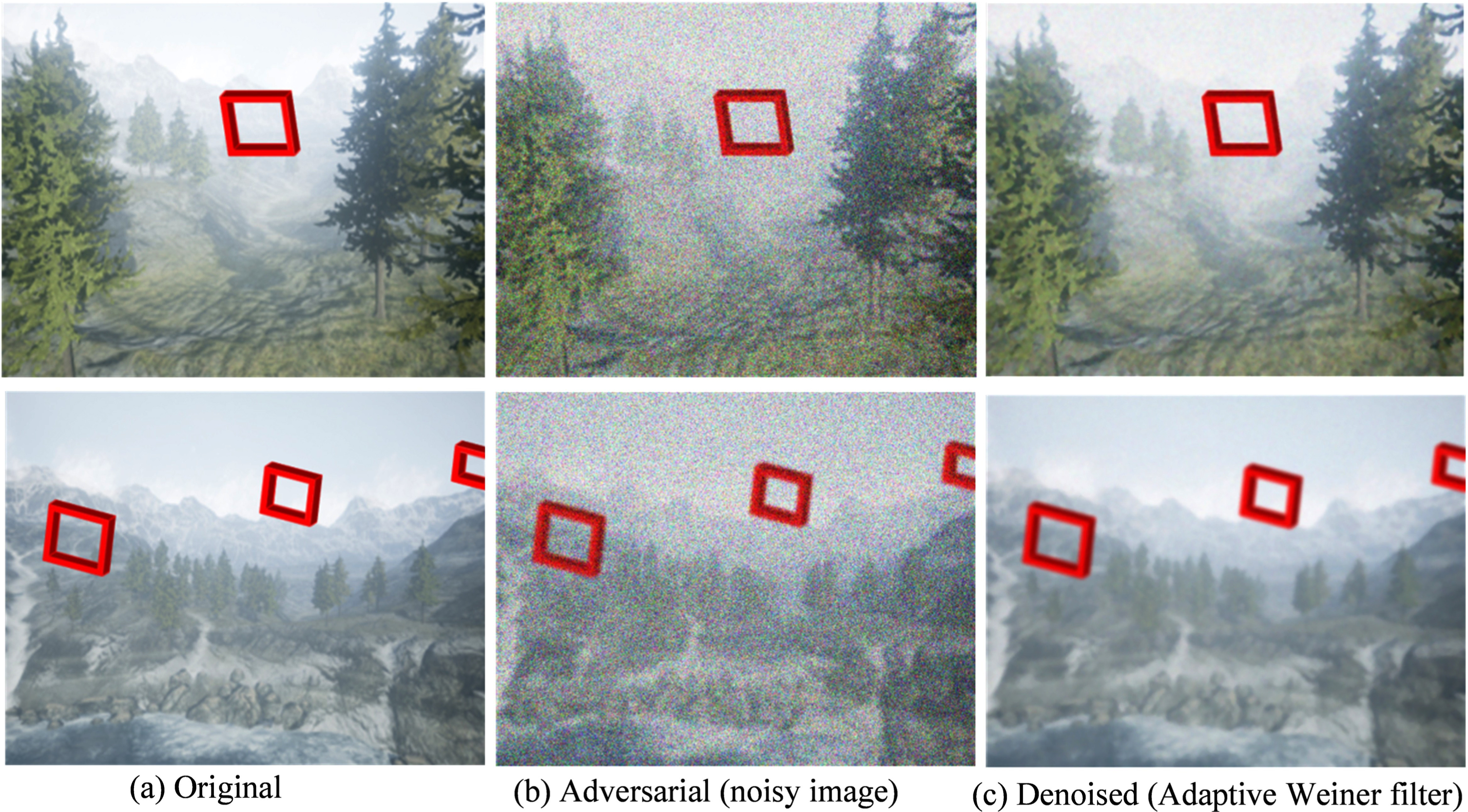
Representation of denoised images using adaptive Weiner filter.

3.3 W-MobileNet framework

In this section, an elaboration on the modification of the inherited DCNN model is given. The MobileNet has a computation per epoch of 31 seconds and a total of 28 layers comprising depth-wise and pointwise convolutions followed by batch normalization and ReLU activation. An Average Pooling layer convolves on the extracted features and is then fed to an FC layer and a softmax layer for classification. The following modifications are introduced, and justification for such changes resulting in the proposed W-MobileNet is given.

3.3.1 Stem block

The adaptive Weiner filter is fused as a stem block, and as already explained, its purpose is to denoise frames before the modified DCNN of W-MobileNet starts convolving on the training data. It must be noted that the stem block is not affected by backpropagation during training; as such, the W-MobileNet can be seen as a framework and not a classical DCNN model.

3.3.2 Spatial Separable convolution

The inherited model (MobileNet) uses depthwise separable convolution, which conceptually is a two-stage operation. First, a channel-wise convolution on each channel (RGB) is performed (i.e., 3 × 3 ×1_RGBchannels). Afterward, a 1 × 1 ×3 point-wise convolution linearly integrates the outputs from the channel-wise convolution. Although depthwise convolution in MobileNet enormously reduces the computational complexity and inference time, we conjecture that it can be further reduced with little or no depreciation in performance by using spatial separable convolutions in place of some of the depthwise layers. The spatial separable convolution merges the two-stage operation in depthwise convolution (the channel-wise and pointwise) into a single-stage; this reduces every two layers (depthwise) in the MobileNet architecture to one layer. Since the Keras framework has both pointwise and depthwise initializer, regularizer, and constraints of separable convolution 2D defined within the same init () function, the implementation is feasible.

3.3.3 Shallowing the network

Again, since some repetitive layers in MobileNet do not significantly contribute to the model’s performance, eliminating such layers is laudable. Therefore, for the five repetitive layers with output shapes, 14 × 14 × 512 is reduced to three. Readers are to refer to Table 1 in reference [2] for in-depth details. The elimination of two repetitive layers reduces the computation complexity and increases the inference time.

3.3.4 Branch FC layers

The final modification is three separate branch FC layers that take convolved features from the average pooling layer. Each branch is responsible for estimating one of the three needed navigational control inputs (position, orientation, and speed). Each branch has a softmax layer for classification and a linear regressor for regression. In addition to the modifications, the Swish activation function is utilized [30], while batch normalization is maintained as in MobileNet.

Next, the working principle of W-MobileNet is explained. A 224 × 224 × 3 image goes through the stem block of W-MobileNet (there is no downsampling operation in the stem block). After denoising, the image goes through the second module of the W-MobileNet framework (the modified MobileNet). Here downsampling takes effect using a stride of 2 within the first convolutional layer and the first four sequential Depthwise layers. Lastly, an average pooling is applied on the output dimension of 7 × 7, converted into a one-dimensional vector, and then fed to the three branches of the fully connected layers. During training, W-MobileNet is fed with images and the associated labels, which are sets of positions in North, East, and Down (NED), orientations in quaternions rather than rotational matrix due to computational complexity and UAV drifts, and speed. An example of the associated labels is as follows: $\begin{matrix} {position}_{x, y, z} = \pm {, [45 - 90], \\ [90 - 135] \dots [315 - 360]} \end{matrix}$ $\begin{matrix} {orientation}_{roll, pitch, yawn} = \pm {[0^{\circ} - 45^{\circ}], \\ [45^{\circ} - 90^{\circ}], [90^{\circ} - 135^{\circ}] \dots [315^{\circ} - 360^{\circ}]} \end{matrix}$ $\begin{matrix} speed = {[0_{m / s} - 3_{m / s}], [3_{m / s} - 6_{m / s}], \\ [6_{m / s} - 9_{m / s}] \dots [21_{m / s} - 24_{m / s}]} \end{matrix}$

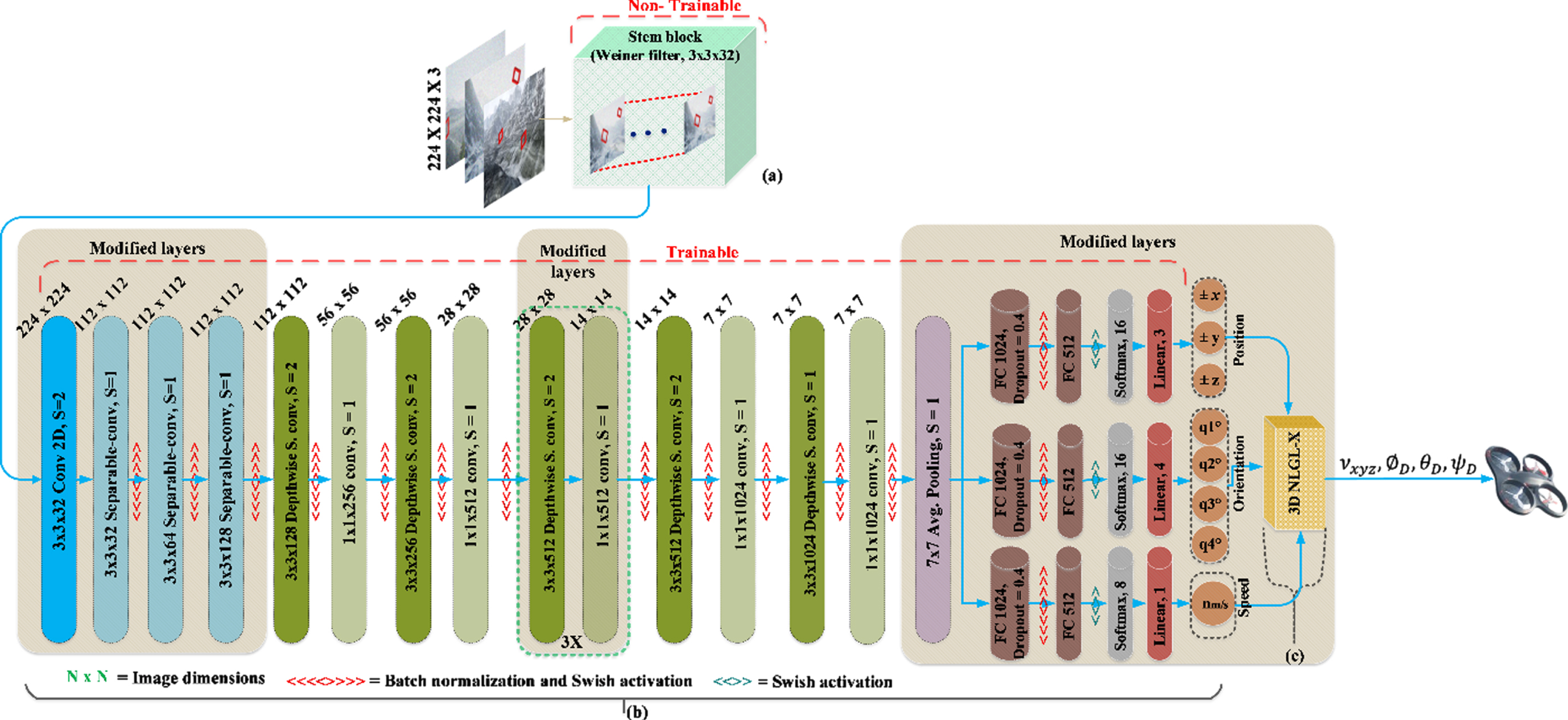
As suggested in [26], orientation in quaternions within the AirSim simulator is much more stable. A quaternion constitutes a four-vector value out of which there are real and complex elements. A quaternion can be expressed as a sum of a scalar q₀ and a vector q = (q₁, q₂, q₃) as: $q = q_{0} + q = q_{0} + q_{1}^{a} + q_{2}^{b} + q_{3}^{c}$ (4) where q₁, q₂, and q₃ are real elements and superscript a = (1, 0, 0) , b = (0, 1, 0) and c = (0, 0, 1) are complex elements, more insight can be deduced from unit quaternion vectors. Using the softmax layer, branch 1 predicts a tuple of positions, and the tuple with the highest probability is selected (e.g., [90 - 135]). Afterward, the linear regressor layer performs regression for specific positional values (e.g., x = 115, y = 94, andz = 131). It should be noted that all the regressed estimations fall within the tuple prediction from the softmax layer. Branches 2 and 3, responsible for orientation and speed estimation, go through the same procedure as branch 1. Figure 3 represents the schematic of the W-MobileNet framework.

Fig. 3

A complete framework of W-MobileNet: (a) denotes the adapted Weiner filters for image restoration, (b) represents the modified MobileNet for feature extraction and inference making, and (c) illustrates the modified 3D-NLGL for streamlining navigational commands. Best seen at a zoom resolution > 140%.

3.4 W-MobileNet integration with 3D NLGL-X

In [4], with some limitations, a two-dimensional (2D) NLGL algorithm is modified to work in a three-dimensional space. Briefly, the NLGL algorithm uses the Virtual Target Point (VTP), which is an imaginary point on the desired path L, (i.e., L is the distance between the UAVs current position and the desired destination) to move the UAV via periodic updates/iterations. In [4], the author’s modification requires feeding the 3D-NLGL with the current vehicle (UAV) position (x, y, z), the yaw (ψ), the distance L and the desired velocity V_path of the vehicle in the x body frame of the vehicle using a constant speed. The algorithm then returns velocities in x, y, and z directions, with z representing their altitude and the yaw angle ψ for rotation. From the algorithm description given, there is a limitation in orientation (no roll and pitch). Again, a constant speed is used in deriving velocities in x, y, and z directions, and the velocity derived in z direction is substituted directly to get the altitude. Although the approach used in [4] to gain altitude is feasible, desirably, flying vehicles gain altitude via orientation by pitching up/down based on some velocity. Based on the limitations outlined, this study extends the 3D-NLGL algorithm in [4] from now on 3D-NLGL-X to output orientations in the aspect of roll, yaw, and pitch, velocities in x, y, and z directions derived from alternating speed. As such, the UAV has six degrees (up, down, left, right, forward, and back) of freedom of movement within a three-dimensional space, see Fig. 4 for visual insight.

Fig. 4

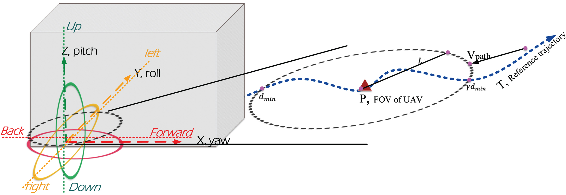
Graphical insight into the 3D-NLGL-X.

First, the drag force acting on the UAV is taken into consideration. Assuming the drag force acting on the UAV in all weather conditions in the virtual environment is calculated as: $F_{d} = C_{d} \times 0.5 (ρ \times v^{2} \times A)$ (5) where F_d is the drag force, C_d is the drag coefficient of the UAV, ρ is the density of the weather, v is the flow velocity of the weather, and A is the area of the UAV. The drag coefficient C_d of the UAV is set at an inclination of 0⁰, 25⁰, and 45⁰ as 0.045, 0.065, and 0.900 respectively. Once the drag force F_d is computed, the required thrust power required for the UAV to overcome the drag force is calculated as: $T_{p} = F_{d} \times v_{m / s}$ (6) where v_m/s is the predicted speed from the W-MobileNet and T_p is the thrust power (velocities) to propel the UAV in the desired x, y, and z directions and orientations (i.e., T_p ≅ V_path on line 11 of Algorithm 1). The 3D-NLGL-X algorithm takes in the current position P : (x, y, z) , orientation Q : (∅ , θ, ψ) of the UAV, the desired destination V_path (i.e., predicted position, orientation, and speed from the W-MobileNet. It should be noted that the predicted speed is integrated with Equation 6 to generate velocities) and a constant scalar L. γ_prev represents γd_min in the previous iteration of Algorithm 1, γ_prev is set to 0 during the first iteration of Algorithm 1. As explained, 3D-NLGL is based on VTP. In Algorithm 1, VTP is computed from lines 15 to 21. The computation starts by calculating two possible intersections d_min and γd_min given by γf (i.e., γf is the x, y, z coordinate on the imaginary circle drawn using the scalar/radius L) from the reference trajectory. Afterward, the VTP (γVPT) is set in the direction of the reference trajectory if the distance d_min is greater than distance L or the projected V_path on the imaginary circle else, the VTP (γVPT) is computed as given on line 21 of Algorithm 1. The projection of V_path from space onto the imaginary circle ensures the UAV moves nearly on the same reference trajectory. A graphical insight is given in Fig. 4.

From lines 22 to 28 in Algorithm 1, the required orientation roll ∅_D, pitch ∅_D, and yaw ψ_D, which must be ⩽π to aline the UAV with the selected γVPT is computed. We found this experimentally efficient as it allows smooth orientation movement in small intermittent angles rather than swift angle rotation. On line 28 of Algorithm 1, the required velocity, which is set proportional to dVPT_x,y,z, projection in the xyz plane about the distance L contrary to xy plane as in [4] is computed. The return of Algorithm 1, as seen on line 29, is sent as the navigational commands (line 30) to the UAV, where the commands are integrated with the Inertial Measurement Unit (IMU) of the quadrotor (UAV), and the UAV updates its position.

3.5 Adaptive weighted loss

DCNN/CNN models are trained using optimization algorithms that require loss functions to update the model’s weights via backpropagation to minimize the loss associated with the model’s next prediction. In DCNN/CNN regression tasks, the Mean Squared Error (MSE), which computes the average squared differences between a model’s predictions and the ground truth (actual instances/values), is the preference. However, since MSE succumbs to outliers in data, squaring the residual magnifies the error when the difference between the prediction and the actual is high. As a result, when the weights of a DCNN/CNN model are nearing perfection during training, an outlier may disrupt the nearly perfect weights due to the magnified error; this leads to the less robustness of the MSE as compared to the Mean Absolute Error (MAE) which is less stable. To this end, the Adaptive Weighted Loss (ADWL) is proposed in this study. ADWL is given as: $ADWL = \frac{1}{n} \sum_{i = 1}^{n} {(D)}^{2}$ (7) where n denotes the total number of data points in the dataset and $D = (Y_{i} - {\tilde{Y}}_{i}) \pm l$ . Here $Y_{i} - {\tilde{Y}}_{i}$ is the actual difference between the predictions ${\tilde{Y}}_{i}$ and the ground truth Y_i and l is the loss after each iteration/epoch during training. Ideally, the adaptive weight is 0 < l < n, where n is the highest loss, usually after the first iteration/epoch. Before the training, the value of l is unknown, l takes an initializer l_i = 0.1, …, 0.5 for the first iteration. The loss l as well as the initializer l_i is added if the difference in the prediction $(Y_{i} - {\tilde{Y}}_{i})$ is below the actual instance/value else subtracted if the difference is higher than the actual instance. The adaptive weight l aims to minimize the difference between the predicted and the actual prior squaring to minimize the magnified error, thereby relaxing the penalty when the difference between the actual and predicted is big.

By definition, ADWL is the squared difference of the actual difference between the predicted and the actual plus or minus the adaptive weight, which initially is set to an initializer l_i = 0.1, …, 0.5 and subsequently replaced with the loss l after each iteration/epoch. Figure 5 shows the losses of the W-MobileNet framework trained with the proposed loss function ADWL and the existing loss functions (MSE, MAE, MSLE, and MBE). From Fig. 5, using ADWL results in early convergence and spikes reduction, which correlates to abrupt changes in the near-perfect weights of W-MobileNet during training. Among the existing cost functions (MSE, MAE, MSLE, and MBE), MSE shows a much more competitive performance; however, the spiky nature of MSE is a challenge.

Fig. 5

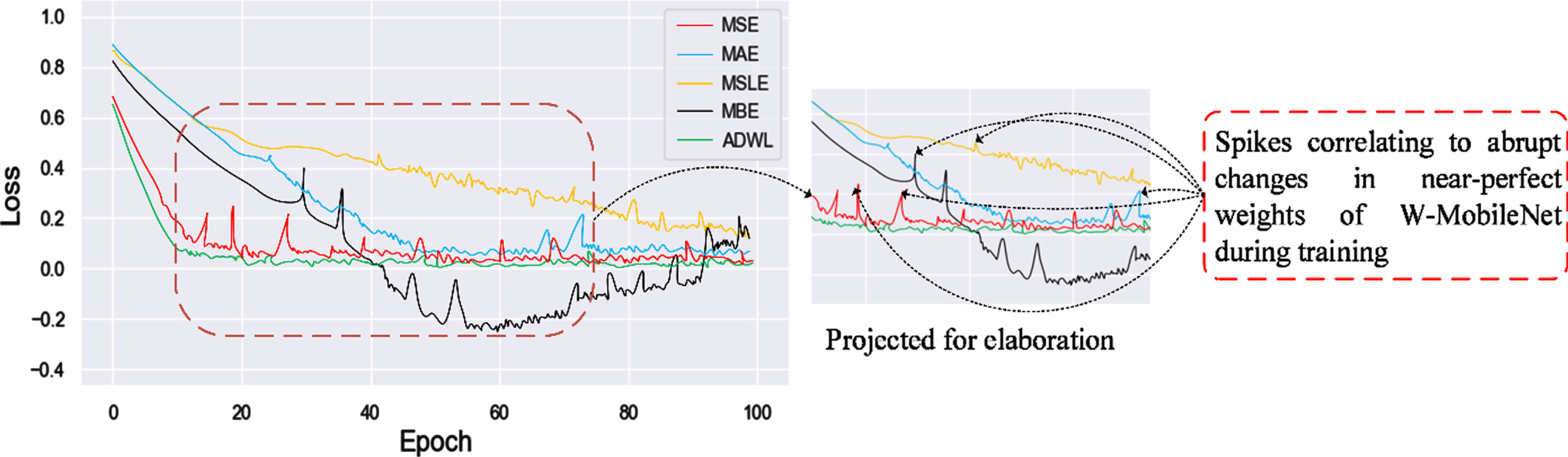
Loss comparison for ADWL and state-of-the-art loss functions used in training of W-MobileNet.

In Table 2, dummy data is utilized to give further elaboration. It can be seen that the MSE penalizes the significant errors, as seen from row 2, whereas ADWL relaxes the penalty on significant errors. On the other hand, MAE does not penalize significant errors (directly proportional to the residual). Also, it does not take into consideration the negative residuals, which leads to the less stable nature of the MAE. The MBE also tends to run into negatives, as seen from rows 1 and 2, thereby going beneath the global minimum (0). Lastly, the MSLE treats small and large residuals nearly the same as in rows 1 and 2.

Table 2

Synopsis analysis of AWDL and existing loss fuctions on a dummy data

Row	Actual	Predicted	MSE	MAE	MSLE	MBE	ADWL (l = 0.5)
Row 1	20	30	100	10	0.0286	–10	90.25
Row 2	20000	30000	100,000,000	10,000	0.0310	–10000	99,990,000
Row 3	30	20	100	10	0.0286	10	90.25
Row 4	30000	20000	100,000,000	10,000	0.0310	10,000	99,990,000

4 Experiment

A simulated and real-world experiment with varying evaluation metrics is carried out to evaluate W-MobileNet and compared with the reference trajectory in addition to the following comparators:

A Multi-Task Regression-based Learning (MTRL) method which adapts the architecture of the Siamese network and predicts positions and orientations; refer to Fig. 2 in [31] for graphical insight.

An Iterative Learning Controller (ILC) encapsulated with a feedback PD controller for stability [32]; this is a non-neural network. The ILC is a well-established control strategy for non-linear systems (e.g., robotic systems). Again the ILC is an intelligent control methodology that utilizes historical data to improve its subsequent predictions/actions; this operational principle has similarities with DCNN models since DCNN models also use historical data prior to predictions.

An ablated W-MobileNet herein MobileNet-X. MobileNet-X is without the stem block, modification to the backbone modular, and integration with the 3D-NLGL-X; hence the difference in performances between W-MobileNet and MobileNet-X denotes the improvements W-MobileNet offers.

4.1 Simulated experiment, setup, and W-MobileNet training

Virtual verification is via the Microsoft AirSim platform built on Unreal Engine, which provides a realistic synthetic 3D environment. W-MobileNet is built as a top layer controller on the simulator using AirSim APIs. Figure 6 illustrates the basic structure of the simulation platform.

Fig. 6

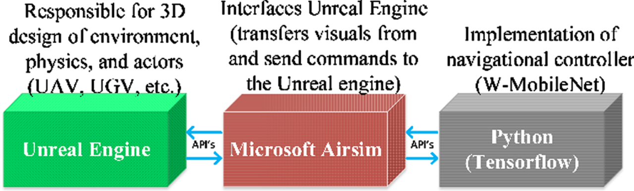
Schematic of the simulation platform.

Data is resized to 224 × 224 × 3 and pre-processed using channel mean-subtraction to center the data. The channel mean-subtraction allows each feature to have a similar range. As such, a single global learning rate multiplier is enough (i.e., during backpropagation, the gradient does not go out of range). Since W-MobileNet performs both classification and regression, for loss functions, categorical-cross entropy is used for classification (Softmax layer in Fig. 3) and the newly proposed loss function AWDL for regression (Linear layer in Fig. 3). Further, equal loss weights were used. 80% of the normalized data is fed to the W-MobileNet for training to commence. W-MobileNet is trained for 100 epochs using a batch size of 64, a learning rate of 0.0001, which controls the step along the gradient, and over time, the Adam optimizer is used to reduce the learning rate progressively. During testing, a copy of the training data (80% used during training) is heavily augmented and added to the unseen 20% of testing data to attain a whole flight trajectory. To ensure the most diversified testing environment, the UAV is set off in an anticlockwise direction of the trajectory rather than clockwise during data collection. In addition, environmental factors (weather conditions) are activated in the Airsim. The computing resource for the experiment is equipped with Nvidia GeForce RTX 2070 with a memory of 16GB running on windows 10 Pro.

4.2 Results and discussion for simulated experiment

An extensive evaluation based on the metrics (i) trajectory performance and time-series analysis, (ii) Hausdorff distance, (iii) cross-track error, and (iv) a quantitative measure (time to complete the trajectory, total distance covered, and the number of successful gateways completed) are used to evaluate the effectiveness, robustness, reliability, and shortcomings of W-MobileNet and the comparators. The experiment is repeated twice under three weather conditions, (i) clear, (ii) rainy/foggy, and (iii) snowy. The intensity of rainy/foggy weather is set to 0.55, and that of snowy is 0.75. Throughout the three weather conditions, an alternating windy condition of 0m/s to 20m/s expressed in the NED directions in the Airsim is maintained.

4.2.1 Trajectory performance and time-series analysis

The trajectory performance evaluates how best each method guides the UAV to follow the reference path. Figures 7a, 7b, and 7c represent trial 1 of the experiment under the three weather conditions (clear, rainy/foggy, and snowy). As seen from trial 1 in Fig. 7a, W-MobileNet mimics the reference trajectory with nearly no track deviation. In clear weather, W-MobileNet exhibits better perceptual knowledge of the environment and can freely navigate with six degrees of freedom; as such, it can follow the reference track effortlessly. Both MTRL and ILC performance is relatively better than the MobileNet-X, which experiences minimum drifts in clear weather conditions. In the rainy/foggy weather of trial 1, the W-MobileNet outperforms the comparators, as seen in Fig. 7b. It can be seen that W-MobileNet gains a slightly higher altitude from the onset. Still, it quickly declines to the optimal altitude and trails the reference trajectory regardless of the environment’s state. Further, navigation under MobileNet-X is challenging, as seen in Fig. 7b. The UAV experiences continuous drifts, circles, and hovers for a short period. The MTRL-based approach initially drifts heavily from the reference trajectory, and about halfway through the track, it starts to converge with the reference trajectory. Such can be said for the ILC method, which improves halfway through the course.

Fig. 7

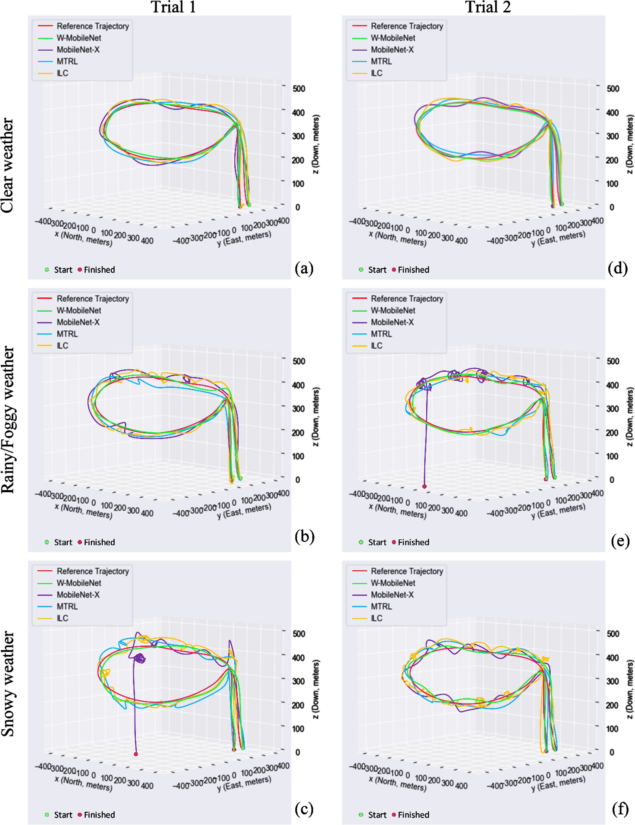
Trajectory performances for the navigational controllers in varying weather conditions in trials 1 and 2, respectively.

Figure 7c depicts the performance of the W-MobileNet trajectory in a snowy environment with an intensity of 0.75; this demonstrates the efficiency of the W-MobileNet configuration. Regardless of the boisterous nature of the snowy environment, which conceptually reduces the visibility of gateways, W-MobileNet denoises the frames, hence attaining a better perception of the environment than the comparators. In Fig. 7c, navigation under the guidance of MobileNet-X, ILC, and MTRL is heavily affected by drifts, circling, and hovering almost throughout the trajectory due to poor perception. Among the comparators, MobileNet-X is unable to complete the entire course. The UAV lands due to long periods of hovering and circling almost at the same place. The conclusion drawn here is that MobileNet-X has an erroneous visual percept of the environment and also fails to generalize; hence its predictions result in the hovering/circling behavior of the UAV. The experiment is repeated for a second round, trial 2. As seen from Figs. 7d, 7e, and 7f, a similar interpretation can be deduced from trial 1; hence further elaboration is not given.

Time series is used to analyze the performance of each navigational controller (W-MobileNet, MobileNet-X, ILC, and MTRL) to gain more insight. For brevity and the assertion that trial 2 trajectory performances of the navigational controllers have similarities with that of trial 1, time series analysis for trial 1 only is given; refer to Figs. 8a, 8b, and 8c, respectively. In Figs. 8a, 8b, and 8c, from top to down, is the visualization of time series analysis in x, y, and z directions for the three varying environments accordingly. Here, the vertical axis denotes the offset in x, y, and z directions, and the horizontal axis is a normalized time for the recorded data points at each gateway. From the perspective of a stochastic model in time series analysis, observations closer in time are much more related than observations farther apart. Subsequently, Figs. 8a, 8b, and 8c show that W-MobileNet has a closer relationship with the reference trajectory than the comparators in all the environment scenarios. Thence, W-MobileNet can be said to be an effective and efficient autonomous navigational controller, arguably in the setting of UAV flight controllers.

Fig. 8

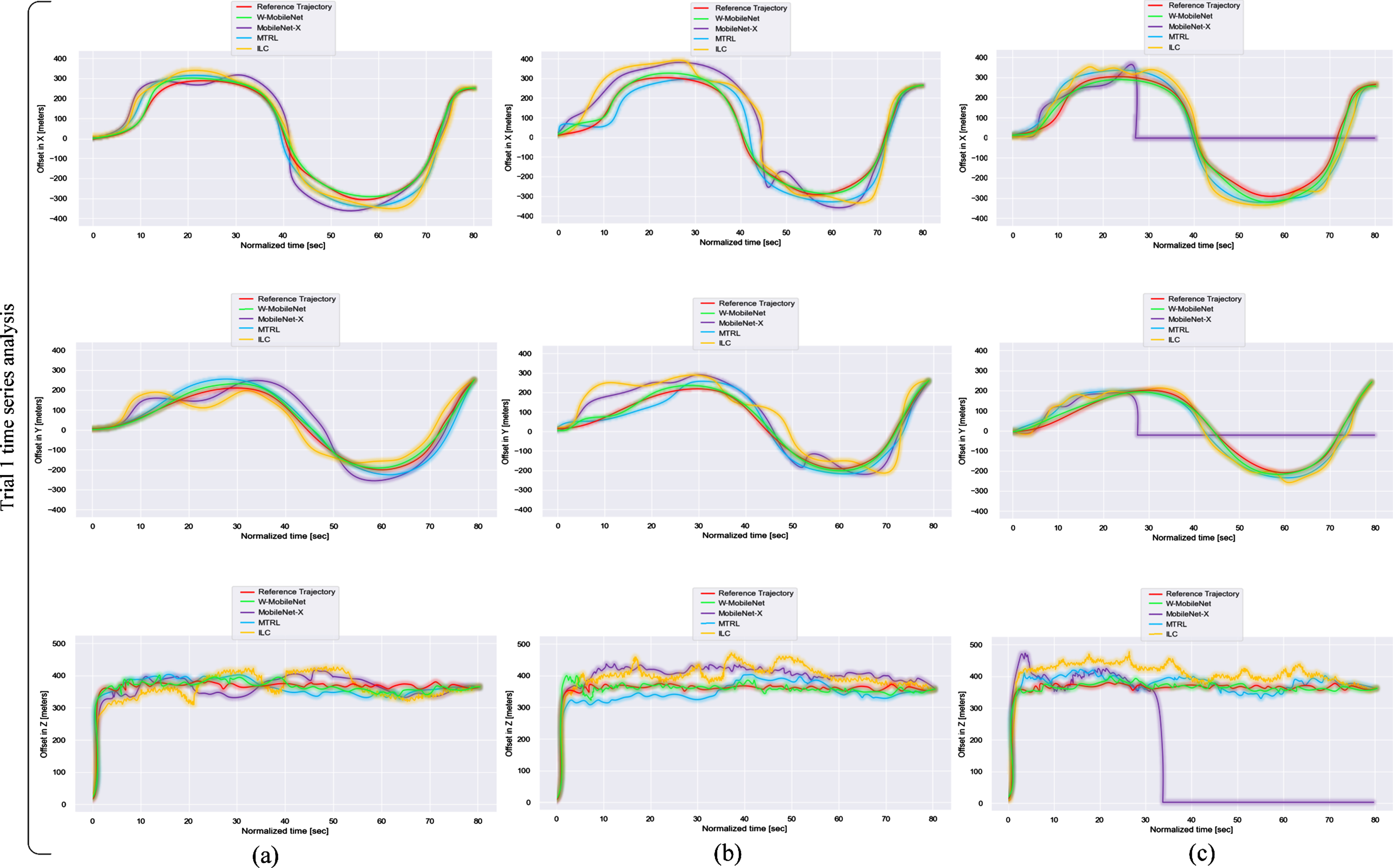
Time series analysis for the UAV navigational controllers in trial 1 of the simulated experiment.

4.2.2 Hausdorff distance

Since the trajectories obtained under the guidance of each navigational controller belongs to the same metric space (M, d) and share similar views; a pairwise distance measure, the Hausdorff distance [33, 34], is employed to compute how far each trajectory is contained within the reference trajectory and vice-versa. The Hausdorff distance is expressed as: $d_{H} (X, Y) = \inf {ɛ ⩾ 0; X \subseteq Y_{ɛ} and Y \subseteq X_{ɛ}}$ (8) where X and Y are two trajectories being compared (i.e., they are non-empty subsets of a metric space where X denotes the reference trajectory and Y take in turns trajectories adduced under each navigational controller). inf is the infimum, ɛ is an epsilon, a fattening parameter for trajectory X and Y where: $X_{ɛ} \sim = \underset{x \in X}{⋃_{\underset{︸}{}}} {z \in M; d (z, x) ⩽ ɛ}$ (9)

That is the set of all points within ɛ of trajectory X . Trajectory Y is also fattened, as in Equation 9. A tabulation of the Hausdorff distance between the reference trajectory and the trajectories adduced under the navigational controllers is given in Table 3. No values for the reference trajectory are provided since it is approximately equal to that of the navigational controllers’ Hausdorff distances.

Table 3

Results of the Hausdorff distance in the simulated experiment

No. of	Navigational	Clear	Rainy/Foggy	Snowy
repetition	controller	weather	weather	weather
Trial 1	Reference trajectory	–	–	–
	W-MobileNet	3.65m	3.75m	6.62m
	MobileNet-X	11.91m	13.05m	12.43m
	MTRL	9.44m	11.92m	10.93m
	ILC	10.32m	12.80m	10.85m
Trial 2	Reference trajectory	–	–	–
	W-MobileNet	2.72m	4.85m	7.24m
	MobileNet-X	15.44m	13.15m	13.35m
	MTRL	9.91m	11.85m	9.35m
	ILC	11.24m	12.51m	9.04m

In Table 3, the lower the Hausdorff distance, the closer the two trajectories being compared. For clarity, the Hausdorff distance between the reference trajectory and W-MobileNet is used to give more insight. From Table 3, under trial 1 of the clear weather environment, the Hausdorff distance between the reference trajectory and that of W-MobileNet is 3.65m . The former implies when the width of the reference trajectory is thickened or widened by 3.65m, the trajectory adduced under the W-MobileNet controller will be contained within the reference trajectory and vice-versa. As seen from Table 3, trajectories adduced under the W-MobileNet controller are relatively close to that of the reference trajectory due to precision in control. As such, W-MobileNet attains the lowest Hausdorff distances compared to the comparator controllers.

4.2.3 Cross-Track-Error

The Cross-Track-Error (XTE) is defined as the instantaneous vertical deviation of the UAV either to the left or right side of the reference trajectory (i.e., XTE is to determine the lateral position of the UAV regarding the reference trajectory). To compute XTE, a vector ${\vec{V}}_{n}$ is defined concerning the reference trajectory plane containing the waypoints/gateways. The vector ${\vec{V}}_{n}$ is considered to be standard, and it is expressed as: ${\vec{V}}_{n} = {\hat{v}}_{1} \times {\hat{v}}_{2}$ (10) where ${\hat{v}}_{n}$ is a unit vector along $\vec{V}$ . During simulation, at time t₊₁, if the UAV position vector is ${\vec{P}}_{n}$ , then the computation of XTEis given as: $XTE = - {\vec{P}}_{n} \times {\hat{V}}_{n}$ (11)

From Fig. 9, the XTE for W-MobileNet under the three varying environmental conditions in both experiment repetitions is better than the comparators. Regardless of the deviation on both sides of the reference trajectory (deviation on the left and right side of the path), it can be seen that W-MobileNet converges quickly with the reference trajectory. In all environmental scenarios of the simulated experiment, the XTE for W-MobileNet declines quickly and reaches zero. However, sometimes, due to swift changes in orientation, the XTE momentarily increases, but W-MobileNet quickly puts the UAV back on the reference path; hence the XTE for W-MobileNet is nearly zero. The capability of W-MobileNet to mitigate the XTE almost to zero is attributed to the 3D-NLGL-X modular.

Fig. 9

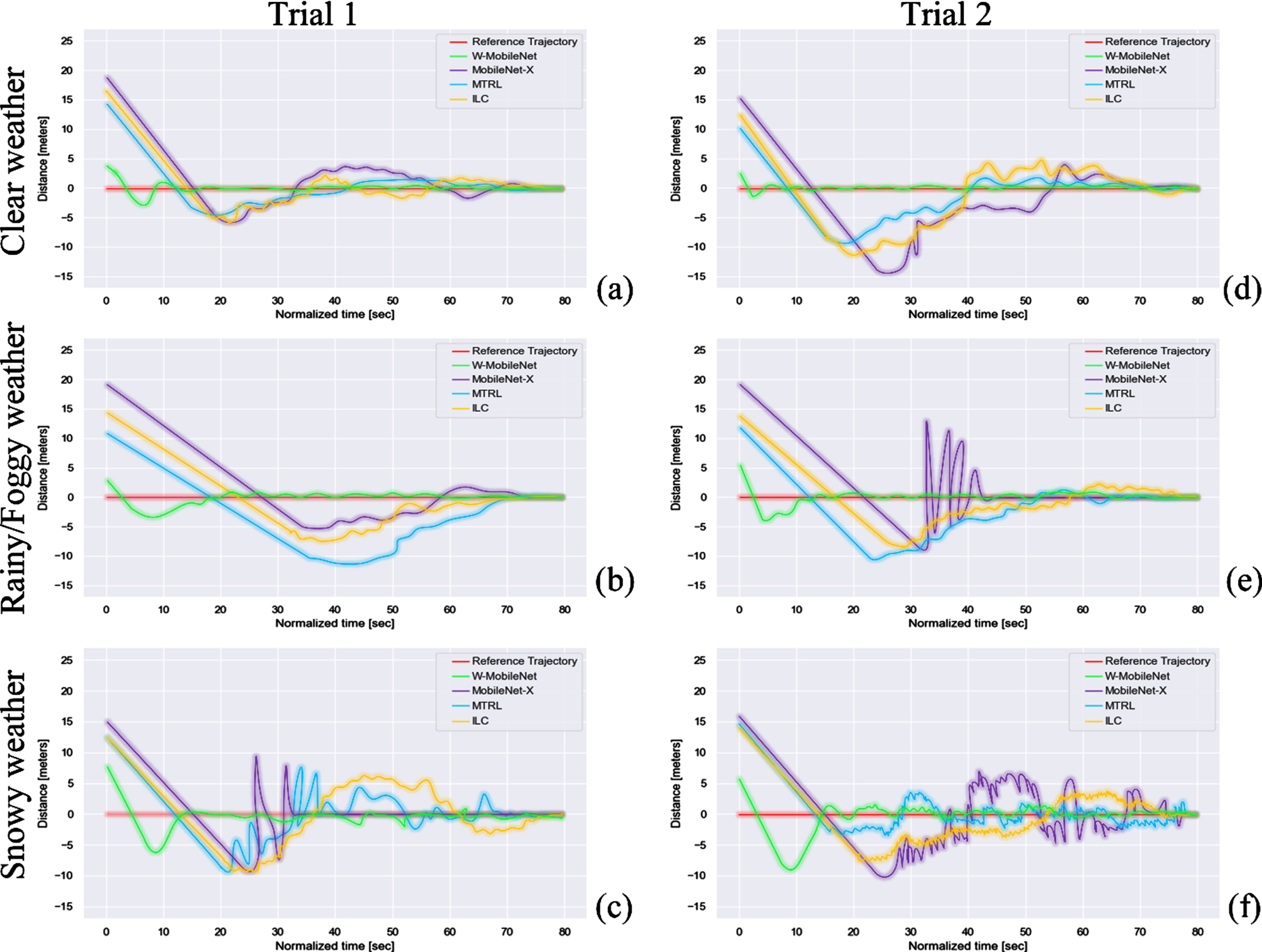
Comparison of cross-track-error between W-MobileNet and the two comparators for trials 1 and 2 of the simulated experiment.

As explained earlier, the 3D-NLGL-X acts as a path planner, enhancing the predictions from the DCNN part of W-MobileNet. By comparing the XTE of the comparators to W-MobileNet, clearly from Fig. 9, under all environmental scenarios, the comparators record higher XTE, and it takes a longer competitive time for the comparators to converge with the reference path. An observation of the large XTE for ILC is due to a gimbal lock, a loss of one degree of movement in three-dimensional space. As a result, the continuous erroneous accumulation of orientation leads to drifts from the reference trajectory, which reflects in the various evaluation metrics for the ILC method. In short, since the W-MobileNet records the least XTE, it takes less time to complete the entire trajectory. A normalized time is used on the x-axis of the sub-figures in Fig. 9 for the representation of the XTE for comparative reasons. The actual times to complete the trajectories are given under the quantitative measure metric under sub Section 4.2.4.

4.2.4 Quantitative measure

To analyze the quantitative performance of each navigational controller, the time taken to complete the trajectory, the total distance covered, and the number of gateways completed are used. Distances between two gateways are used to calculate the time taken to travel between the two. Assuming the path between two gateways G₁ and G₂ is straight with positional vectors $\vec{V}$ and $\vec{U}$ , then the distance D_t between the two vectors $\vec{V}$ and $\vec{U}$ is computed as: $D_{t} (\vec{V}, \vec{U}) = \sqrt{{({\hat{v}}_{1} - {\hat{u}}_{1})}^{2} + {({\hat{v}}_{2} - {\hat{u}}_{2})}^{2}}$ (12) where ${\hat{v}}_{n}$ and ${\hat{u}}_{n}$ are unit vectors. Given v_m/s to be the speed of the UAV, then the time T_t taken to complete the trajectory from start to end is given as: $T_{t} = \frac{D_{t}}{v_{m / s}}$ (13)

Table 4 gives a numerical insight into the performance of each navigational controller. Based on the number of gateways completed in all varying weather scenarios and repetitions of the experiment, W-MobileNet exhibits much better robustness than MTRL, ILC, and MobileNet-X. W-MobileNet completes at least 35 out of 50 gateways (refer to Table 4, trial 1 of snowy weather) and 46 out of 50 gateways at most (refer to trial 1 of clear weather). In addition, the time taken to complete the trajectory and total distance covered is satisfactory compared to that of MTRL, ILC, and MobileNet-X in both experiment repetitions in the clear and rainy/foggy weather scenarios, respectively. From Table 4, the most challenging scenario is that of the snowy weather environment. Here the number of gateways completed reduces for all navigational controllers compared to those achieved in clear and rainy/foggy weather. The time and total distance covered are also worse than the results in the clear and rainy/foggy environments except for MobileNet-X in trial 1 of rainy/foggy weather, where it records a time of 26 min 31sec and a distance of 919.41m. The disparities in the duration and total distance reached by the four navigators in the two repetitions of the experiment are ascribed to the airflow to overcome and the UAV’s behavior (hovering, circling, and deviation from the reference trajectory).

Table 4

Numerical insight into the performance of each navigational controller for the simulated experiment

Clear Weather
	Trial 1			Trial 2
Navigational controller	Time	Total distance covered	Gateway completed	Time	Total distance covered	Gateway completed
Reference trajectory	12min 19sec	750m	50 out of 50	12min 19sec	750m	50 out of 50
W-MobileNet	13min 06sec	752.54m	46 out of 50	13min 02sec	751.21m	44 out of 50
MobileNet-X	19min 48sec	812.03m	29 out of 50	17min 52sec	789.04m	32 out of 50
MTRL	17min 08sec	793.31m	32 out of 50	15min 38sec	763.24m	28 out of 50
ILC	17min 21sec	788.44m	34 out of 50	16min 03sec	771.24m	27 out of 50
Rainy/Foggy Weather
Reference trajectory	12min 19sec	750m	50 out of 50	12min 19sec	750m	50 out of 50
W-MobileNet	13min 58sec	757.13m	41 out of 50	14min 07sec	763.44m	39 out of 50
MobileNet-X	26min 31sec	919.41m	13 out of 50	28min 32sec	394.31m	6 out of 50
MTRL	20min 02sec	821.34m	17 out of 50	19min 47sec	802.23m	24 out of 50
ILC	21min 46sec	848.21m	15 out of 50	23min 51sec	871.04m	16 out of 50
Snowy Weather
Reference trajectory	12min 19sec	750m	50 out of 50	12min 19sec	750m	50 out of 50
W-MobileNet	15min 27sec	771.08m	35 out of 50	15min 09sec	766.21m	37 out of 50
MobileNet-X	10min 21sec	203. 35m	4 out of 50	21min 34sec	809.32m	11 out of 50
MTRL	21min 38sec	844.07m	17 out of 50	17min 22sec	791.45m	19 out of 50
ILC	23min 09sec	819.24m	19 out of 50	24min 05sec	803.14m	20 out of 50

A secondary observation centered much on the reliability of each navigational controller is to understand the correlation between the time, total distance, and gateways completed. From Table 4, results under clear weather, W-MobileNet achieved more gateways in trial 1 compared to the gateways completed in trial 2. Yet, in trial 2, W-MobileNet has better results for the time and total distance covered than in trial 1. Similarly, in the most challenging scenario, the snowy weather environment, MobileNet-X records presumably the best time (10 min 21sec) during trial 1, refer to Table 4. However, it fails to complete the trajectory (refer to Fig. 7c for graphical insight), recording 203.35m and completing 4 out of 50 gateways. The discrepancies between the results under time, the total distance covered, and the number of gateways completed for the repetition of the experiment make it quite challenging to assess the reliability of each navigational controller. To this end, the mean of each sub-evaluation metric (time, total distance covered, and gateway completed) for trials 1 and 2 in all three weather scenarios are computed. The results are summarized in Table 5. Based on Table 5, it is evident that W-MobileNet has more substantial reliability than MTRL, ILC, and MobileNet-X. It should be noted that the average distance covered by MobileNet-X even falls short of that of the reference trajectory since it did not complete the entire course twice, refer to Fig. 7c and 7e.

Table 5

Summarized results of the numerical performance of the navigational controllers for the simulated experiment

Navigational controller	Avg. time	Avg. total distance covered	Avg. gateway completed
Reference	12min 19sec	750m	50 out of 50
trajectory
W-MobileNet	14min 01sec	760.26m	40 out of 50
MobileNet-X	20min 53sec	654.57m	16 out of 50
MTRL	18min 42sec	802.60m	23 out of 50
ILC	20min 08sec	816.88m	22 out of 50

4.3 Real-world experiment with DJI Tello drone

The real-world experiment is designed to answer the following research questions: (i) What are the transferability and generalization capabilities of W-MobileNet from simulation to reality? (ii) Can W-MobileNet be deployed on a physical drone? (iii) How well can W-MobileNet handle real-world trajectories layout?

4.3.1 Setup

DJI Tello is used, a low-cost programmable drone that runs on an Intel 14-core processor and shoots at 720p with a 5-megapixel at a frame rate of 30fps. First, two reference trajectories are obtained from an expert user flying the DJI Tello drone on a circular and rectangular track using the GameSir T1d Controller. The adduced reference trajectories are used as a benchmark to assess the performance of W-MobileNet alongside the comparators (MTRL, ILC, and MobileNet-X). The two trajectories mentioned before are characterized by varying challenges (straight segments, swift elevation changes, and hairpin curves). Fabricated gateways measured 100cm × 100cm were used at vantage waypoints of the two reference trajectories refer to Fig. 10c. The fabricated gateways aid in visualizing the reference trajectories/tracks since they are imaginary in reality and serve as an evaluation metric.

Fig. 10

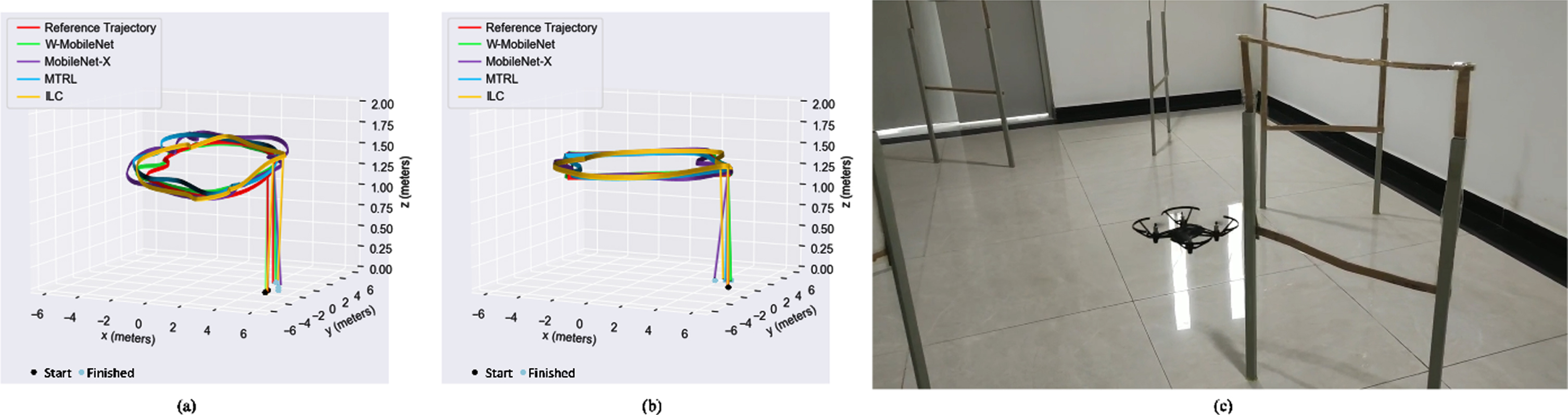
Trajectory performance by each navigational controller in the real-world experiment.

All three DCNN models acting as navigational controllers follow a similar training and testing approach as in sub-Section 4.1. In response to the question of transferability and generalization, the last convolutional layer of W-MobileNet is retrained for geometric feature specifics of the real-world trajectories. The learned weights from the simulated experiment (circle trajectory) are used as initializers. The same training modification is applied to the two DCNN comparators. Since the DJI Tello drone is a low-resource constrained edge node, the compute resource stated in sub-Section 4.1 is utilized during the retraining and testing the navigational controllers. However, the question of deploying W-MobileNet on a physical drone is partially answered since the drone acts in the real environment based on the navigational commands received from W-MobileNet running on a computer. The last question, which is centered on the performance of W-MobileNet in particular in the real environment, is answered using the experimental results, which are evaluated on three axes: (i) trajectory performance, (ii) Hausdorff distance, and (iii) gateways completed. Unless otherwise noted, 6 and 4 fabricated gateways are used in the circle and rectangular trajectories, respectively.

4.3.2 Results and discussion for real-world experiment

The isometric trajectory performance of the navigators is shown in Figs. 10a and 10b. On a scale of 100%, we conjecture W-MobileNet achieves a track performance rate of about 90% and 93% for the circle and rectangular trajectories, respectively, factoring in all the challenges associated with both reference trajectories. MobileNet-X, an ablated navigational controller to W-MobileNet, shows the worst performance.

Based on the trajectories performance as shown in Figs. 10a and 10b, there is much more improvement in trajectory performance due to the configuration of the W-MobileNet framework, which: (i) denoises the From left to right: (a) circular trajectory performance, (b) rectangular trajectory performance, and (c) a composite scene from the real-world experiment.frames, as such significant features are learned, and (ii) integrates navigational estimates with the 3D-NLGL-X, leading to intuitive and precision control of the UAV. The MTRL and ILC methods perform averagely on both reference trajectories competitively, and both are relatively better than the MobileNet-X method but lag behind W-MobileNet. Table 6 summarizes the numerical performance of the navigators under evaluation metrics Hasudorf distance and gateways completed. Complimentary, a conjectured trajectory performance rate is also given in Table 6, and Fig. 10c shows a composite scene during the real-world experiment. Readers can refer to the video in [35] for visual insight into the performance of W-MobileNet. Although we fancy an overall success rate of 91.5% for W-MobileNet for both trajectories, some minimum drifts during the real-world experiment are acknowledged. Presumptuously, the drifts observed in the real-world experiment possibly could be attributed to a calibration error of the DJI Tello drone

Table 6
Real-world numerical results for insight into the performance of the navigational controllers

Navigational controller Hausdorff distance Gateways completed Conjectured trajectory rate

Circle Rectangle Circle Rectangle Circle Rectangle Overall

Reference trajectory – – 6 out of 6 4 out of 4 100% 100% 100%

W-MobileNet 0.43m 0.16m 6 out of 6 4 out of 4 90% 93% 91.5%

MobileNet-X 1.31m 0.64m 4 out of 6 4 out of 4 79% 85% 82%

MTRL 0.64m 0.25m 5 out of 6 4 out of 4 88% 90% 89%

ILC 0.71m 0.59m 4 out of 6 4 out of 4 82% 89% 85.5%

Navigational controller	Hausdorff distance	Gateways completed	Conjectured trajectory rate
Reference trajectory	–	–	6 out of 6	4 out of 4	100%	100%	100%
W-MobileNet	0.43m	0.16m	6 out of 6	4 out of 4	90%	93%	91.5%
MobileNet-X	1.31m	0.64m	4 out of 6	4 out of 4	79%	85%	82%
MTRL	0.64m	0.25m	5 out of 6	4 out of 4	88%	90%	89%
ILC	0.71m	0.59m	4 out of 6	4 out of 4	82%	89%	85.5%

5 Conclusion and future work

This study implements a new hybrid method for the autonomous vision-based UAV trajectory trial task. The hybrid approach is segmented into three main modules: (i) a denoising mechanism, (ii) the perceptual awareness of DCNN, and (iii) the precision mechanism of a path planner. Integrating the three modules, as mentioned before, resulted in a UAV navigational controller termed W-MobileNet, which continuously predicted navigational commands regarding position coordinates, orientation, and speed for the UAV. Further, a novel loss function characterized by a weighting mechanism was utilized in training W-MobileNet, resulting in faster convergence. The pros and cons of the proposed hybrid navigational controller were investigated extensively from a simulation perspective and a real-world experiment utilizing a micro aerial drone. Based on the evaluation metrics: (i) trajectory track performance and time series analysis, (ii) Hausdorff distance, (iii) cross-track-error, and (iv) a numerical quantitative measure, the findings of the experiments indicate W-MobileNet is favorable in terms of precision and robustness over the state-of-the-art methods, a non-neural network method, and an ablated W-MobileNet.

Although the potential of W-MobileNet as a UAV navigational controller takes us a step closer to autonomous UAV applications, scaling the presented approach to applications such as package delivery would always require the partial intervention of a human pilot due to the unknown path. In addition, W-MobileNet lacks a UAV calibration error mechanism; as such, the two critics, as mentioned earlier, would be a direction to look into in future research.

Footnotes

Acknowledgment

This work was partly supported by the National Natural Science Foundation of China under Grants 61571099 and 61501098.

The authors thank Lui Zhang and Joshua Offeh Beakoh for aiding the real-world experiments and Priscilla Fosu Sarkodie and Abigail Boamah for extensive proofreading. Also, the authors are grateful for the helpful advice from Dr. Brigther Agyemang, Samuel Osei Agyemang, and Micheal Osei Agyemang.

A video of the real-world experiment is available at the given link:

References

Agyemang

I.O.

, Zhang

, Acheampong

, Adjei-Mensah

, Kusi

G.A.

, Mawuli

B.C.

and Agbley

B.L.Y.

, Automation in Construction Autonomous health assessment of civil infrastructure using deep learning and smart devices, Autom Constr 141 (September) (2022), pp. 104396, https://doi.org/10.1016/j.autcon.2022.104396.

Howard

A.G.

et al., MobileNets: Efficient Convolut ional Neural Networks for Mobile Vision Applications, 2017, [Online]. Available: http://arxiv.org/abs/1704.04861.

Vaseghi

S.V.

“Wiener Filters,”Vieweg+Teubner Verlag, In Advanced Signal Processing and Digital Noise Reduction (1996). doi: org/10.1007/978-3-322-92773-6_5.

Rubí

, Pérez

and Morcego

, A Survey of Path FollowingControl Strategies for UAVs Focused on Quadrotors, J IntellRobot Syst Theory Appl 98(2) (2020)pp. 241–265. doi: 10.1007/s10846-019-01085-z.

Agyemang

I.O.

, Zhang

, Adjei-Mensah

, Arhin

J.R.

and Agyei

, Lightweight Real-time Detection of Components via a Micro Aerial Vehicle with Domain Randomization Towards Structural Health Monitoring, Period Polytech Civ Eng 66(2) (2022)pp. 516–531. doi: https://doi.org/10.3311/ppci.18689. Torresan

et al., Forestry applications of UAVs in Europe: a review, Int J Remote Sens 38(8–10) (2447)pp. 2427–2447. doi: 10.1080/01431161.2016.1252477.

Chen

M.Y.

et al., Designing a spatially aware and autonomousquadcopter, 2013 IEEE Syst Inf Eng Des Symp SIEDS 2013 (2013)pp. 213–218. doi: 10.1109/SIEDS.2013.6549521.

, He

, Huynh

, Corke

Monocular vision-based autonomous navigation for a cost-effective MAV in GPSdenied environments, 2013 IEEE/ASME Int Conf Adv Intell Mechatronics Hum Wellbeing, AIM 2013, pp. 1355–1360, 2013, doi: 10.1109/AIM.2013.6584283.

Zhang

, Microsoft Kinect sensor and its effect, IEEEMultimed 19(2) (2012)pp. 4–10. doi: 10.1109/MMUL.2012.24.

Roberts

S.Z.

, Floreano Quadrotor Using Minimal Sensing For Autonomous Indoor Flight, Proc Eur Micro Air Veh Conf Flight Compet EMAV2007, vol. 07, no. September, pp. 1–8, 2007, [Online]. Available: http://infoscience.epfl.ch/record/111485/files/Roberts-MAV07.pdf.

10.

Cruz

G.C.S.

and Encarnacão

P.M.M.

, Obstacle avoidance for unmanned aerial vehicles, J Intell Robot Syst Theory Appl 65(1–4) (2012)pp. 203–217. doi: 10.1007/s10846-011-9587-z.

11.

Bachrach

et al., Estimation, planning, and mapping for autonomous flight using an RGB-D camera in GPS denied environments, The Int Jour of Rob Res 31(11) 2012. https://dx-doi-org.web.bisu.edu.cn/10.1177/0278364912455256.

12.

Vandapel

, Kuffner

and Amidi

, Planning 3-D path networks in unstructured environments, Proc - IEEE Int Conf Robot Autom 2005no. May (2005)pp. 4624–4629. doi: 10.1109/ROBOT.2005.1570833.

13.

Bry

, Bachrach

, Roy

State estimation for aggressive flight in GPS-denied environments using onboardsensing, Proc - IEEE Int Conf Robot Autom, (2012), pp. 1–8, doi: 10.1109/ICRA.2012.6225295.

14.

Bachrach

, De Winter

, He

, Hemann

, Prentice

, Roy

, RANGE - Robust autonomous navigation in GPS-denied environments, Proc - IEEE Int Conf Robot Autom (2010), pp. 1096–1097, doi: 10.1109/ROBOT.2010.5509990.

15.

Zhang

, Kahn

, Levine

and Abbeel

, Learning deep control policies for autonomous aerial vehicles with MPC-guided policy search, Proc - IEEE Int Conf Robot Autom 2016 (2016)pp. 528–535. doi: 10.1109/ICRA.2016.7487175.

16.

Fang

, Xu

, Wang

and Zeng

, Target-driven visual navigation in indoor scenes using reinforcement learning and imitation learning,pp. –, CAAI Trans Intell Technol 1 (2021)pp. 3357–3364. doi: 10.1049/cit2.12043.

17.

Passalis

and Tefas

, Continuous drone control using deep reinforcement learning for frontal view person shooting, Neural Comput Appl 32(9) (2020)pp. 4227–4238. doi: 10.1007/s00521-019-04330-6.

18.

Wang

, Wang

, Shen

and Zhang

, Autonomous Navigation of UAVs in Large-Scale Complex Environments: A Deep Reinforcement Learning Approach, IEEE Trans Veh Technol 68(3) (2019) pp. 2124–2136. doi: 10.1109/TVT.2018.2890773.

19.

Hwangbo

, Sa

, Siegwart

and Hutter

, Control of a Quadrotor with Reinforcement Learning, IEEE Robot Autom Lett 2(4) (2107)pp. 2096–2103. doi: 10.1109/LRA.2017.2720851.

20.

Agyemang

I.O.

, Zhang

, Acheampong

, Adjei-Mensah

, Gyamfi

E.O.

, Ayivi

, Amuche

C.I.

RPNet : Rotational Pooling Net for Efficient Micro Aerial Vehicle Trail Navigation, SSRN, 2022, [Online]. Available: https://dx-doi-org.web.bisu.edu.cn/10.2139/ssrn.4095698.

21.

Smolyanskiy

, Kamenev

, Smith

, Birchfield

Toward low-flying autonomous MAV trail navigation using deep neural networks for environmental awareness, IEEE Int Conf Intell Robot Syst, vol. 2017-Septe, pp. 4241–4247, 2017, doi: 10.1109/IROS.2017.8206285.

22.

Maciel-Pearson

B.G.

, Carbonneau

and Breckon

T.P.

, Extending deep neural network trail navigation for unmanned aerial vehicle operation within the forest canopy,LNAI, Lect Notes Comput Sci (including Subser Lect Notes Artif Intell Lect Notes Bioinformatics) 10965 (2018)pp. 147–158. doi: 10.1007/978-3-319-96728-8_13.

23.

Kelchtermans

, Tuytelaars

How hard is it to cross the room? –Training (Recurrent) Neural Networks to steer a UAV, no. February 2017, 2017, [Online]. Available: http://arxiv.org/abs/1702.07600.

24.

Giusti

et al., A Machine Learning Approach to Visual Perception of Forest Trails for Mobile Robots, IEEE Robot Autom Lett 1(2) (2016)pp. 661–667. doi: 10.1109/LRA.2015.2509024.

25.

Martinez

, Sampedro

, Chauhan

, Campoy

Towards autonomous detection and tracking of electric towers for aerial power line inspection, 2014 Int Conf Unmanned Aircr Syst ICUAS 2014 - Conf. Proc (2014), pp. 284–295, doi: 10.1109/ICUAS.2014.6842267.

26.

Shah

, Dey

, Lovett

and Kapoor

, AirSim: High-Fidelity Visual and Physical Simulation for Autonomous Vehicles, Springer Proc Adv Robot 5 (2018)pp. 621–635. doi: 10.1007/978-3-319-67361-5_40.

27.

Madaan

et al., AirSim Drone Racing Lab,” no. Il, pp. 177–191, 2020, [Online]. Available: http://arxiv.org/abs/2003.05654.

28.

Agyemang

I.O.

AirSim Landscape 1007 Mountains V1, Science Data Bank, [Online], Available: https://www.scidb.cn/en/s/eA3euy.

29.

, Yang

, Xiao

and Zhu

, Adaptive wiener filter and natural noise to eliminate adversarial perturbation, Electron 9(10) (2020)pp. 1–14. doi: 10.3390/electronics9101634.

30.

Ramachandran

, Zoph

, Le

Q.V.

Searching for activation functions, 6th Int Conf Learn Represent (2018), pp. 1–13, [Online]. Available: https://openreview.net/forum?id=Hkuq2EkPf.

31.

Maciel-Pearson

B.G.

, Akcay

, Atapour-Abarghouei

, Holder

and Breckon

T.P.

, Multi-Task Regression-Based Learning for Autonomous Unmanned Aerial Vehicle Flight Control Within Unstructured Outdoor Environments, IEEE Robot Autom Lett 4(4) (2019)pp. 4116–4123. doi: 10.1109/lra.2019.2930496.

32.

, Hu

, Shen

, Kong

, Zhao

, Yao

An iterative learning controller for quadrotor UAV path following at a constant altitude, Chinese Control Conf CCC, vol. 2015-Septe, no. Section 2 (2015), pp. 4406–4411, doi: 10.1109/ChiCC.2015.7260322.

33.

Tyrrel

R.R.

, Roger

J.B.W.

Variational Analysis, Springer-Verlag., pp. 117, 2005, ISBN 3-540-62772-3, 2005.

34.

Birsan

, Tiba

One Hundred Years Since the Introduction of the Set Distance by Dimitrie Pompeiu, In Ceragioli F., Dontchev A., Futura H., Marti K., Pandolfi L. (eds) System Modeling and Optimization.CSMO2005. IFIP International Federation for Information Processing, vol 199. Springer, Boston, MA, doi.org/10.1007/0-387-33006-2_4..

35.

Agyemang

I.O.

Accelerating Trial NAvigation for UAV Experiment, YouTube, [Online], Available: https://youtu.be/m7KWFa1rH3U.