Feature selection for interval-valued data via FRIC -model

1 Introduction

Rough set theory (RST) is a significant method to handle uncertainty. Its idea is to use the known knowledge to describe the uncertain knowledge. An information system (IS) was presented by Pawlak [30, 31]. RST can effectively deal with the uncertainty of an IS. The application of RST is mostly related to an IS [25, 43].

In real life, some data are expressed in the form of interval-valued numbers, such as estimating the price of an item, the age of a person, the length of a sample, etc. Thus, interval-valued data is an important type of data. An interval-valued information system (IVIS) means an IS where its attribute values are interval-valued numbers. When the conditional attribute values of a decision information system (DIS) are interval-valued numbers, it is called an interval-valued decision system (IVDIS). IVISs and IVDISs are regarded as the generalization of IS and DIS, respectively, which can describe imprecise samples more accurately. Some scholars have studied IVISs and IVDISs. For example, Dai et al. [9] studied uncertainty measurement for an IVDIS via extended conditional entropy; Zhang et al. [43] presented incremental updating of rough approximations in an IVIS under attribute generalization; Xie et al. [37] considered new measurements of uncertainty for an IVIS; Liu et al. [23] proposed attribute reduction algorithm via the fuzzy α-similarity relation in an incomplete IVIS.

Feature selection as an important technology of data processing in machine learning can effectively reduce redundant selections and improve the accuracy of classification. According to feature selection process whether relys on the learner, feature selection methods are usually divided into three categories: filtered [21], wrapped [20] and embedded [18]. Feature selection of RST can delete redundant attributes of conditional feature set while maintaining the dependency between conditional attributes and decision attributes in a decision table. It is a filtered feature selection method. Many researchers studied feature selection. Dai et al. [8] presented attribute attribute via conditional entropies for an incomplete DIS. Zhao et al. [44] put forward mixed feature selection in an incomplete DIS. Chen et al. [1] introduced a fuzzy kernel-feature selection method for heterogeneous data. Jia et al. [19] proposed similarity-based feature selection in RST from clustering perspective. Hu et al. [16] presented a robust and fast feature selection method on the basis of separability for a fuzzy DIS. Wang et al. [34] explored feature selection by means of local conditional entropy.

Fuzzy rough set (FRS) was proposed by Dubois et al. [6]. Moresi et al. [26] presented the axiomatic definition for FRS. Cornelis et al. [2] considered feature selection with FRS. Chen et al. [4] gave an feature selection algorithm based on FRS. Hu et al. [17] developed kernelized FRS. Wang et al. [35] investigated feature selection with FRS. Yuan et al. [40] studied unsupervised feature selection for mixed data based on FRS. Thippa et al. [33] discussed two of the prominent dimensionality reduction techniques. Gadekallu et al. [13] used the improved hybrid bat and firefly algorithms to calculate feature selection. Wang et al. [36] studied feature selection for categorical data based on FRS. The biggest advantage of intelligent algorithm is that it is fast and can deal with all kinds of datasets, but it is difficult to reduce the number of attributes while ensuring the classification accuracy.

Classical rough set model can deal with categorical data. The deficiency of this model is that it is sensitive to noise in classification learning due to the stringent condition of an equivalence relation. Thus, a fuzzy relation is introduced to describe the similarity between samples with categorical data. By the way, FRS model is established to manage feature selection for categorical data.

In order to handle interval-valued data, we usually use “The similarity between information values is fed back to the sample set”. But we can deal with interval-valued data from the perspective of “The similarity between information values is fed back to the feature set". Based on this perspective, a fuzzy relation can be defined to describe the similarity between samples, a variable parameter can be introduced to control the similarity between samples and FRIC-model can be established. This paper studies feature selection for interval-valued data via FRIC-model.

This paper is organized as follows. Section 2 recalls interval-valued numbers and IVDISs, and then introduces the fuzzy symmetry relation induced by each subsystem. Section 3 presents several attribute evaluation functions. Section 4 proposes FRIC-model in an IVDIS. Section 5 gives a feature selection algorithm in an IVDIS via FRIC-model. Section 6 implements comparative analysis. Section 7 executes statistical analysis. Section 8 concludes the paper.

2 Preliminaries

Throughout this paper, O signifies a finite set, 2 ^O denotes the family of all subsets on O, |X| expresses the cardinality of X ∈ 2 ^O ,

Put O = { o 1 , o 2 , ⋯ , o n }(1)

Definition 3.1.Let (O, A, d) be an IVDIS. Given B ⊆ A and θ ∈ [0, 1]. Define S B θ _ ( X ) ( o ) = ⋀ o ′ ∉ X , ∀ o ∈ O(13) S B θ ¯ ( X ) ( o ) = ⋁ o ′ ∈ X S B θ ( o , o ′ ) , ∀ o ∈ O(14) Then S B θ _ ( X ) and S B θ ¯ ( X ) are referred to as the lower and upper fuzzy approximations of X, respectively.

Proposition 3.2.Let (O, A, d) be an IVDIS. Then the following properties hold. (1) ∀ B ⊆ A, ∀ θ ∈ [0, 1], ∀ X ∈ 2 ^O , S B θ _ ( X ) ⊆ X ⊆ S B θ ¯ ( X ) , where X ( o ) = { 1 , o ∈ X ; 0 , o ∉ X . (2) If B₁ ⊆ B₂ ⊆ A, then ∀ θ ∈ [0, 1], ∀ X ∈ 2 ^O , R B 1 θ _ ( X ) ⊆ R B 2 θ _ ( X ) , R B 2 θ ¯ ( X ) ⊆ R B 1 θ ¯ ( X ) .

(3) If 0 ≤ θ₁ < θ₂ ≤ 1, then ∀ B ⊆ A, ∀ X ∈ 2 ^O , R B θ 1 _ ( X ) ⊆ R B θ 2 _ ( X ) , R B θ 1 ¯ ( X ) ⊆ R B θ 2 ¯ ( X ) . Proof.

(1) (i) Given B ⊆ A, θ ∈ [0, 1], X ∈ 2 ^O . Then by Definition 2.9, we can obtain that ∀ o , o ′ ∈ O , 0 ≤ S B θ ( o , o ′ ) ≤ 1 .

This implies that 0 ≤ ⋀ o ′ ∉ X [ 1 - S B θ ( o , o ′ ) ] ≤ 1 .

So ∀ o ∈ O, 0 ≤ S B θ _ ( X ) ( o ) ≤ 1 .

Thus ∀ o ∈ X, S B θ _ ( X ) ( o ) ≤ 1 = X ( o ) .

Note that ∀ o ∉ X, S B θ _ ( X ) ( o ) = ⋀ o ′ ∉ X [ 1 - S B θ ( o , o ′ ) ] ≤ 1 - S B θ ( o , o ) = 0 . Then ∀ o ∉ X, S B θ _ ( X ) ( o ) = 0 ≤ 0 = X ( o ) .

It follows that ∀ o ∈ O, S B θ _ ( X ) ( o ) ≤ X ( o ) .

Thus S B θ _ ( X ) ⊆ X .

(ii) Clearly, ∀ o ∈ O , 0 ≤ S B θ ¯ ( X ) ( o ) ≤ 1 .

Then ∀ o ∉ X, X ( o ) = 0 ≤ S B θ ¯ ( X ) ( o ) .

Note that ∀ o ∈ X, S B θ ¯ ( X ) ( o ) = ⋁ o ′ ∈ X S B θ ( o , o ′ ) ≥ S B θ ( o , o ) = 1 . Then ∀ o ∈ X, S B θ ¯ ( X ) ( o ) = 1 ≤ 1 = X ( o ) .

This implies that ∀ o ∈ O, X ( o ) ≤ S B θ ¯ ( X ) ( o ) .

Thus X ⊆ S B θ ¯ ( X ) .

From the above, S B θ _ ( X ) ⊆ X ⊆ S B θ ¯ ( X ) .

(2) (i) Note that B₁ ⊆ B₂ ⊆ A. Then by Proposition 2.10, R B 1 θ ⊆ R B 2 θ .

So ∀ o ∈ O, o′ ∉ X, R B 1 θ ( o , o ′ ) ≤ R B 2 θ ( o , o ′ ) .

This implies that ∀ o ∈ O, ⋀ o ′ ∉ X [ 1 - R B 2 θ ( o , o ′ ) ] ≤ ⋀ o ′ ∉ X [ 1 - R B 1 θ ( o , o ′ ) ] .

Thus ∀ o ∈ O, R B 2 θ _ ( X ) ( o ) ≤ R B 1 θ _ ( X ) ( o ) .

Therefore, R B 2 θ _ ( X ) ⊆ R B 1 θ _ ( X ) .

(ii) Note that B₁ ⊆ B₂ ⊆ A. Then by Proposition 2.10, R B 1 θ ⊆ R B 2 θ .

This implies that ∀ o ∈ O, o′ ∈ X, R B 1 θ ( o , o ′ ) ≤ R B 2 θ ( o , o ′ ) .

So ⋁ o ′ ∈ X R B 1 θ ( o , o ′ ) ≤ ⋁ o ′ ∈ X R B 2 θ ( o , o ′ ) .

Thus R B 1 θ ¯ ( X ) ( o ) ≤ R B 2 θ ¯ ( X ) ( o ) .

Hence R B 1 θ ¯ ( X ) ⊆ R B 2 θ ¯ ( X ) .

(3) (i) Note that 0 ≤ θ₁ < θ₂ ≤ 1. Then by Proposition 2.10, R B θ 1 ⊆ R B θ 2 .

So ∀ o ∈ O, o′ ∉ X, R B θ 1 ( o , o ′ ) ≤ R B θ 2 ( o , o ′ ) .

This implies that ∀ o ∈ O, ⋀ o ′ ∉ X [ 1 - R B θ 2 ( o , o ′ ) ] ≤ ⋀ o ′ ∉ X [ 1 - R B θ 1 ( o , o ′ ) ] .

Thus ∀ o ∈ O, R B θ 2 _ ( X ) ( o ) ≤ R B θ 1 _ ( X ) ( o ) .

Therefore, R B θ 2 _ ( X ) ⊆ R B θ 1 _ ( X ) .

(ii) Note that B₁ ⊆ B₂ ⊆ A. Then by Proposition 2.10, R B θ 1 ⊆ R B θ 2 .

It follows that ∀ o ∈ O, o′ ∈ X, R B θ 1 ( o , o ′ ) ≤ R B θ 2 ( o , o ′ ) .

So ⋁ o ′ ∈ X R B θ 1 ( o , o ′ ) ≤ ⋁ o ′ ∈ X R B θ 2 ( o , o ′ ) .

Thus R B θ 1 ¯ ( X ) ( o ) ≤ R B θ 2 ¯ ( X ) ( o ) .

Hence R B θ 1 ¯ ( X ) ⊆ R B θ 2 ¯ ( X ) .□

Definition 3.3. Let (O, A, d) be an IVDIS with B ⊆ A and θ ∈ [0, 1]. The fuzzy positive region of decision d relative to B is computed by POS B θ ( d ) = ⋃ D ∈ O / d S B θ _ ( D ) = ⋃ i = 1 r S B θ _ ( D i )(15)

Proposition 3.4. Let (O, A, d) be an IVDIS.

(1) If B₁ ⊆ B₂ ⊆ A, then ∀ θ ∈ [0, 1], POS B 2 θ ( d ) ⊆ POS B 1 θ ( d ) .

(2) If 0 ≤ θ₁ < θ₂ ≤ 1, then ∀ B ⊆ A, POS B θ 1 ( d ) ⊆ POS B θ 2 ( d ) .

Proof. It follows from Proposition 3.2.□ Definition 3.5. Let (O, A, d) be an IVDIS. Suppose B ⊆ A and θ ∈ [0, 1]. Then θ-degree of dependence of d relative to B is computed by Γ B θ ( d ) = | POS B θ ( d ) | n(16)

Proposition 3.6. Let (O, A, d) be an IVDIS.

(1) If B₁ ⊆ B₂ ⊆ A, then ∀ θ ∈ [0, 1], Γ B 2 θ ( d ) ⊆ Γ B 1 θ ( d ) .

(2) If 0 ≤ θ₁ < θ₂ ≤ 1, then ∀ B ⊆ A, Γ B θ 1 ( d ) ⊆ Γ B θ 2 ( d ) .

Proof. It follows from Proposition 3.4.□ Definition 3.7. Let (O, A, d) be an IVDIS. Suppose B ⊆ A, θ ∈ [0, 1] and a ∈ A - B. Then θ-significance of a relative to B about d is computed by sig θ ( a , B , d ) = Γ B θ ( d ) - Γ B ∪ { a } θ ( d )(17)

In this section, we establish FRIC-model in an IVDIS with the help of the iterations of fuzzy positive regions and dependency functions.

Let (O, A, d) be an IVDIS. Given B ⊆ A and θ ∈ [0, 1]. For i = |B|, |B|+1, ⋯ , |A|, denote ( S B θ ) i ( o , o ′ ) = 1 i | B oo ′ θ | ( o , o ′ ∈ O )(18) S B θ _ ( D ) i ( o ) = ⋀ o ′ ∉ D [ 1 - ( S B θ ) i ( o , o ′ ) ] ( D ∈ O / d , o ∈ O )(19) S B θ ¯ ( D ) i ( o ) = ⋁ o ′ ∈ D ( S B θ ) i ( o , o ′ ) ( D ∈ O / d , o ∈ O )(20) POS B θ ( d ) i = ⋃ D ∈ O / d S B θ _ ( D ) i(21) Γ B θ ( d ) i = | POS B θ ( d ) i | n(22) sig θ ( a , B , d ) i = Γ B θ ( d ) i - Γ B ∪ { a } θ ( d ) i ( B ⊆ A , a ∈ A - B )(23)

Theorem 4.1.Let (O, A, d) be an IVDIS. Given B ⊆ A and θ ∈ [0, 1]. Then ∀ D ∈ O/d, ∀ o ∈ O, ∀ i ∈ [|B|, |A|-1], S B θ _ ( D ) i + 1 ( o ) = 1 i + 1 + i i + 1 S B θ _ ( D ) i ( o )(24)Proof. S B θ _ ( D ) i ( o ) = ⋀ o ′ ∉ D ( 1 - 1 i | B oo ′ θ | ) = 1 - ⋁ o ′ ∉ D 1 i | B oo ′ θ | = 1 - 1 i ⋁ o ′ ∉ D | B oo ′ θ | .

Similarly, S B θ _ ( D ) i + 1 ( o ) = 1 - 1 i + 1 ⋁ o ′ ∉ D | B oo ′ θ | .

Then 1 i + 1 + i i + 1 S B θ _ ( D ) i ( o ) = 1 i + 1 + i i + 1 ( 1 - 1 i ⋁ o ′ ∉ D | B oo ′ θ | ) = 1 - 1 i + 1 ⋁ o ′ ∉ D | B oo ′ θ | .

Thus S B θ _ ( D ) i + 1 ( o ) = 1 i + 1 + i i + 1 S B θ _ ( D ) i ( o ) . □

Theorem 4.2.Let (O, A, d) be an IVDIS. Given B ⊆ A and D ∈ O/d. Then ∀ i ∈ [|B|, |A|-1], S B θ ¯ ( D ) i + 1 = i i + 1 S B θ ¯ ( D ) i(25)Proof. Clearly.□

Theorem 4.3.Let (O, A, d) be an IVDIS. Given B ⊆ A and θ ∈ [0, 1]. Then ∀ o ∈ O, ∀ i ∈ [|B|, |A|-1], POS B θ ( d ) i + 1 ( o ) = 1 i + 1 + i i + 1 POS B θ ( d ) i ( o )(26) noindentProof. By Theorem 4.1, we can obtain that ∀ o ∈ O, ∀ i, POS B θ ( d ) i + 1 ( o ) = ⋁ D ∈ O / d S B θ _ ( i + 1 ) ( D ) ( o ) = ⋁ D ∈ O / d ( 1 i + 1 + i i + 1 S B θ _ ( i ) ( D ) ( o ) ) = 1 i + 1 + ⋁ D ∈ O / d i i + 1 S B θ _ ( i ) ( D ) ( o ) = 1 i + 1 + i i + 1 ⋁ D ∈ O / d S B θ _ ( i ) ( D ) ( o ) .

Thus POS B θ ( d ) i + 1 ( o ) = 1 i + 1 + i i + 1 POS B θ ( d ) i ( o ) . □

Theorem 4.4.Let (O, A, d) be an IVDIS. Given B ⊆ A and θ ∈ [0, 1]. Then ∀ i ∈ [|B|, |A|-1], Γ B θ ( d ) i + 1 = 1 i + 1 + i i + 1 Γ B θ ( d ) i(27)Proof. By Theorem 4.3, | POS B θ ( d ) i + 1 | = ∑ i = 1 n POS B θ ( d ) i + 1 ( o i ) = ∑ i = 1 n ( 1 i + 1 + i i + 1 POS B θ ( d ) i ( o i ) ) = 1 i + 1 n + i i + 1 ∑ i = 1 n POS B θ ( d ) i ( o i ) = 1 i + 1 n + i i + 1 | POS B ( i ) ( o i ) | .

Then | POS B θ ( d ) i + 1 | n = 1 i + 1 + i i + 1 | POS B θ ( d ) i | n .

Thus Γ B θ ( d ) i + 1 = 1 i + 1 + i i + 1 Γ B θ ( d ) i . □

Theorem 4.5.Let (O, A, d) be an IVDIS. Suppose B ⊆ A, a ∈ A - B. Then ∀ i ∈ [|B|, |A|-1], sig θ ( a , B , d ) i + 1 = i i + 1 sig θ ( a , B , d ) i(28)Proof. By Theorem 4.4, sig θ ( a , B , d ) i + 1 = Γ B θ ( d ) i + 1 - Γ B ∪ { a } θ ( d ) i + 1 = 1 i + 1 + i i + 1 Γ B θ ( d ) i - ( 1 i + 1 + i i + 1 Γ B ∪ { a } θ ( d ) i ) = i i + 1 Γ B θ ( d ) i - i i + 1 Γ B ∪ { a } θ ( d ) i = i i + 1 ( Γ B θ ( d ) i - Γ B ∪ { a } θ ( d ) i ) .

Thus sig θ ( a , B , d ) i + 1 = i i + 1 sig θ ( a , B , d ) i . □

This part presents an feature selection algorithm in an IVDIS via FRIC-model.

Definition 5.1. Let (O, A, d) be an IVDIS. Given B ⊆ A and θ ∈ [0, 1]. Then B is referred to as a feature selection subset of A to d, if POS B θ ( d ) = POS A θ ( d ) and a ∈ B, a is POS B - { a } θ ( d ) ≠ POS A θ ( d ) .

Algorithm 1 Obtain a feature selection subset in an MSVDIS (FRIC)

REQUIRE An IVDIS (O, A, d), D ∈ O/d, θ, δ.

ENSURE A feature selection subset B.

1: Let n = |O|, B =∅, i = 1;

2: Computer matrix R =(r_oo′) _n×n, where o ∈ D and o′ ∈ O - D, then r_oo′ = 0, otherwise r_oo′ = NaN;

3: for each a ∈ A do

4: foro, o′ ∈ O do

5: Computer S a θ ( oo ′ ) = 1 i | B oo ′ θ | ;

6: end for

7: get each matrix S a θ = ( S a θ ( oo ′ ) ) n × n ;

8: end for

9: i = 0;

10: while true do

11: foreach a ∈ A - B

12: temp = S a θ + R ;

13: foreach D ∈ d

14: Compute R B ⋃ { a k } θ _ ( D ) i ( o ) = min { 1 - 1 i + 1 temp } ;

15: end for

16: Γ B ⋃ { a } θ ( d ) i = | POS B ⋃ { a } θ ( d ) i | n ;

17: end for

18: Find a^* with maximum value Γ B ⋃ { a * } θ ( d ) i ;

19: Compute sig ( a * , B , d ) i + 1 = i i + 1 ( Γ B θ ( d ) i - Γ B ⋃ { a * } θ ( d ) i ;∥

20: if sig(a^*, B, d) _i+1 > δ

21: B = B ∪ {a^*};

22: R = R + S a * θ

23: i = |B|;∥

24: else

25: break;

26: end if

27: end while

28: return B.

Algorithm 1 has a parameter δ, which is a threshold used primarily to control algorithm termination conditions. When the significance of attribute B exceeds δ, the algorithm continues to be executed, and when it is less than δ, the algorithm terminates. Here we analyze the time and space complexity of algorithm 1. The second step is to calculate a matrix, and the time complexity is O(|O|²). The third to eighth steps need to calculate |A| matrices, so the time complexity is O(|A||O|²). The time complexity of steps 10 through 27 is O ( ( | A | + | B | ) 2 * ( | A | - | B | + 1 ) * | O | 2 ) = O ( | A | 2 + | A | - | B | 2 + | B | 2 * | O | 2 ) . Therefore, the time complexity of the whole algorithm is O ( | O | 2 + | A | | O | 2 + | A | 2 + | A | - | B | 2 + | B | 2 * | O | 2 ) = O ( ( | A | 2 - | B | 2 ) * | O | 2 ) . The space complexity of the whole algorithm is O(|A||O|²).

In order to verify the effectiveness of the algorithm, 10 datasets were used for testing. The Fish, car and water are real-life interval-valued datasets [5, 14]. The other seven datasets are real-valued from UCI database [12]. See Table 2 for details of each data set. Since some data are not interval values, they need to be transformed into interval values. We adopted the method in the reference [7]. Let (O, A, d) be an IVDIS. ∀ a ∈ A, o _i  ∈ O, we compute a i - = a i - 2 σ d , a i + = a i + 2 σ d , where σ _d is the standard deviation for the attribute a _i .

Ten graphs are drawn to show the effectiveness of the proposed algorithm and the size change of the reduction set caused by the change of parameters θ and δ. Figures 1-10 shows the curve change of 10 reduced sets obtained by running the FRM-IV algorithm proposed in this paper. The horizontal axis represents the value of δ, from 0 to 0.18. The vertical axis represents the size of the reduction set. Each picture has four curves, and the parameter θ of each curve is 0.6, 0.7, 0.8 and 0.9 respectively. The blue curve represents parameter θ = 0.6, the orange curve represents θ = 0.7, the Yellow curve represents θ = 0.8, and the purple curve represents θ = 0.9. It can be seen from the image that the size of the reduction set decreases with the gradual increase of variable δ for each curve. When θ takes four different values, the downward trend of each curve is close. This shows that the effectiveness of the algorithm is closely related to δ, but it has little to do with θ. In order to find the optimal values of δ and θ, we establish a mathematical model: z = max(δ, θ). z represents classification accuracy. This mathematical model has no explicit expression and is difficult to be solved by the usual method. Therefore, it is solved by the traversal method. First fix the value of δ, and then take the variable θ from 0.5 to 0.99 in steps of 0.01. Adjust the value of δ and traverse θ again. This is repeated until the parameters δ and θ with the maximum classification accuracy are found.

OPEN IN VIEWER

Fig. 1

Reduct (Fish).

OPEN IN VIEWER

Fig. 2

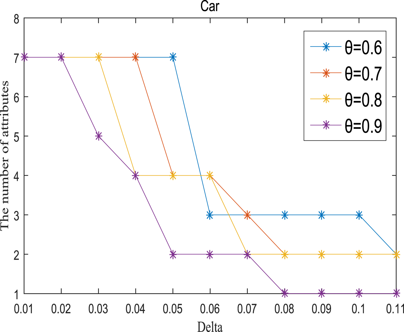
Reduct (Car).

OPEN IN VIEWER

Fig. 3

Reduct (Water).

OPEN IN VIEWER

Fig. 4

Reduct (Ion).

OPEN IN VIEWER

Fig. 5

Reduct (SH).

OPEN IN VIEWER

Fig. 6

Reduct (IS).

OPEN IN VIEWER

Fig. 7

Reduct (Wdbc).

OPEN IN VIEWER

Fig. 8

Reduct (Dia).

OPEN IN VIEWER

Fig. 9

Reduct (Hill).

OPEN IN VIEWER

Fig. 10

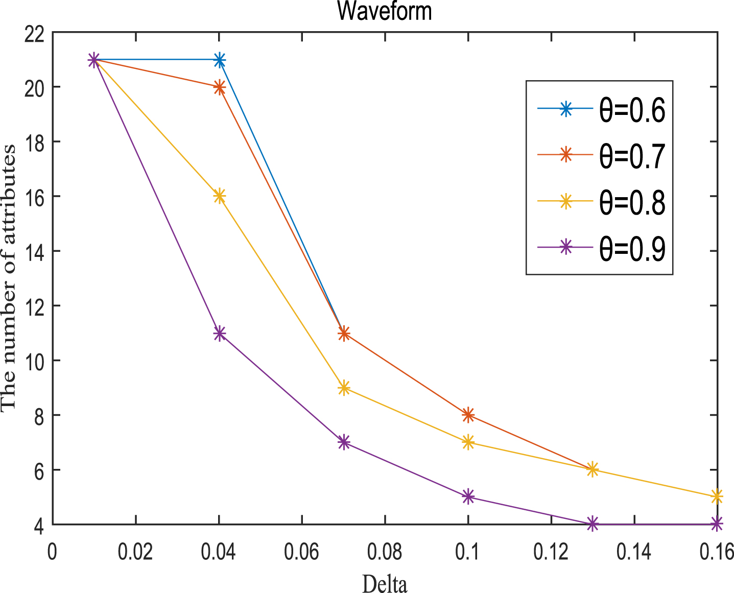
Reduct (Wave).

Next, the accuracy of the algorithm is tested. We randomly select 80% of each data set as the training set and the remaining 20% as the test set. Each data set is trained 10 times, and the accuracy is taken as the average value. Because the current classifiers cannot process real valued datasets, we use the same K-Nearest Neighbor (KNN, K=3) and Probabilistic Neural Network (PNN) classifiers in the reference [7]. The specific formula for measuring the distance between two samples is also shown in the reference [7]. Figures 11-20 show the change of KNN classification accuracy when θ and δ take different values. Figures 21-30 show the accuracy change of classifier PNN when θ and δ take different values. From Figures 11-30, it can be seen that the accuracy curves presented on most images change regularly, and the overall trend increases or decreases gradually. However, it can be clearly seen from Figures 11, 12, 21 and 23, that The four curves on the precision image of datasets fish, car and water vibrate obviously and have no obvious law, indicating that when the δ increases and the reduction set becomes smaller, taking different θ will affect the accuracy of the data set.

OPEN IN VIEWER

Fig. 11

KNN classification accuracy (Fish).

OPEN IN VIEWER

Fig. 12

KNN classification accuracy (Car).

OPEN IN VIEWER

Fig. 13

KNN classification accuracy (Water).

OPEN IN VIEWER

Fig. 14

KNN classification accuracy (Ion).

OPEN IN VIEWER

Fig. 15

KNN classification accuracy (SH).

OPEN IN VIEWER

Fig. 16

KNN classification accuracy (IS).

OPEN IN VIEWER

Fig. 17

KNN classification accuracy (Wdbc).

OPEN IN VIEWER

Fig. 18

KNN classification accuracy (Dia).

OPEN IN VIEWER

Fig. 19

KNN classification accuracy (Hill).

OPEN IN VIEWER

Fig. 20

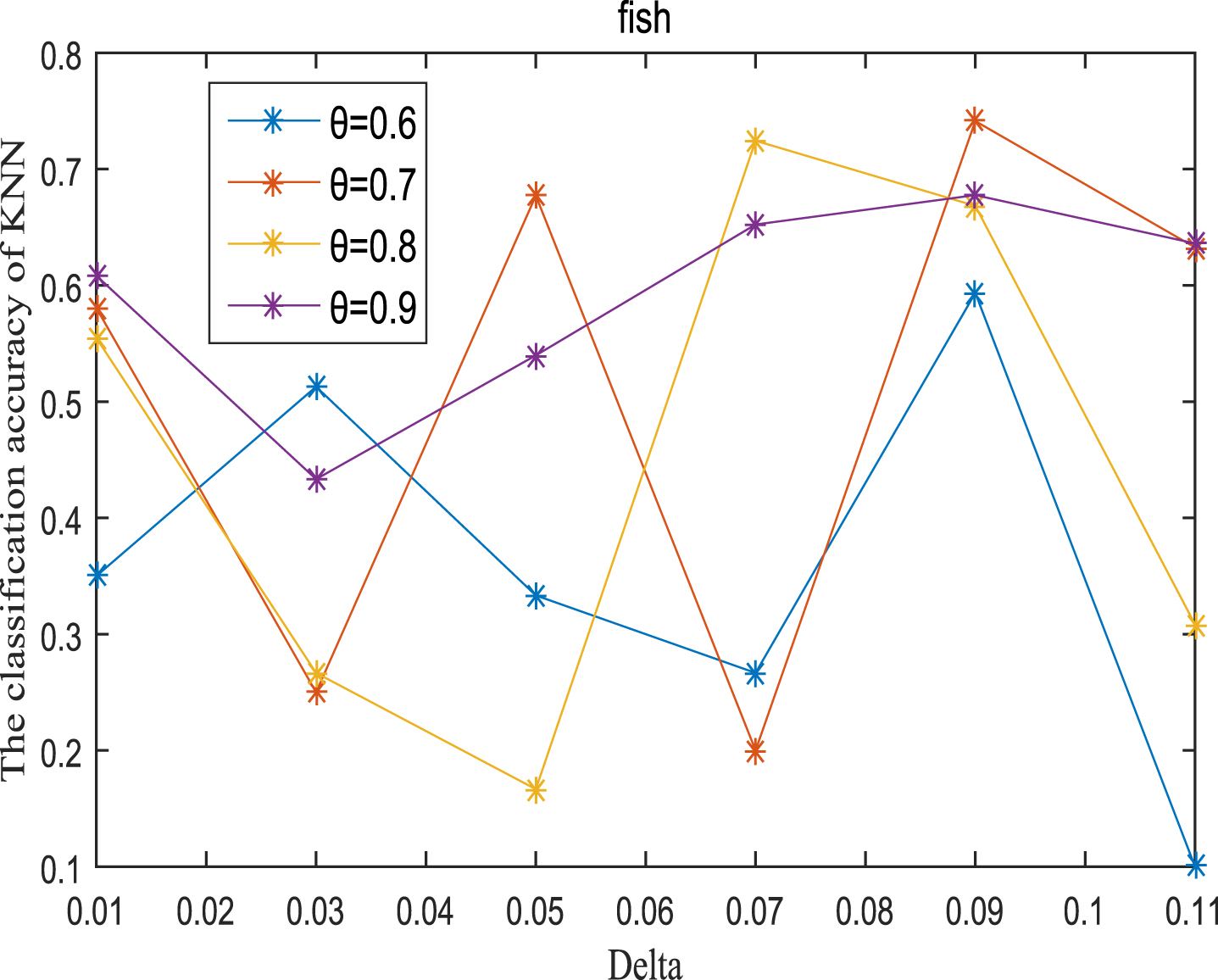
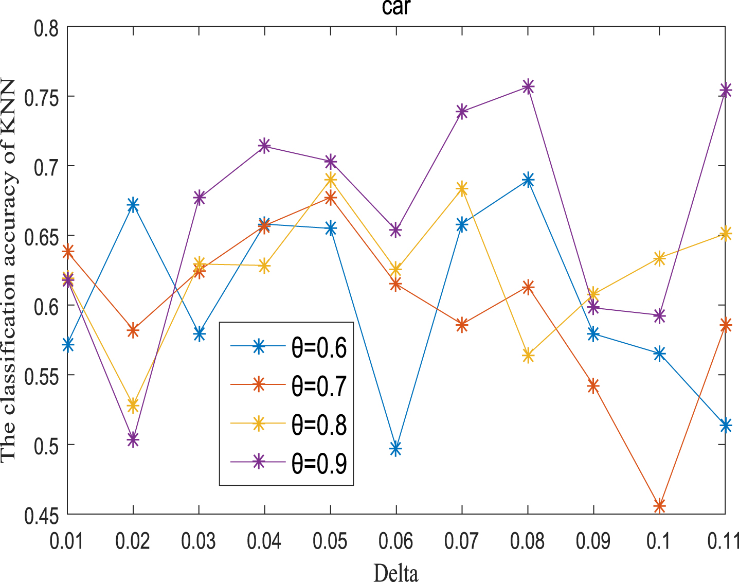
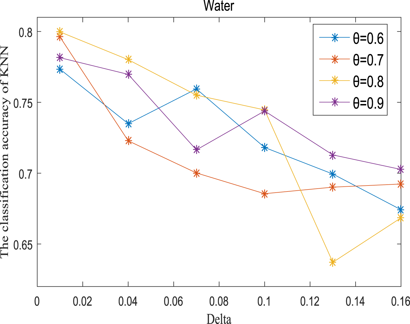
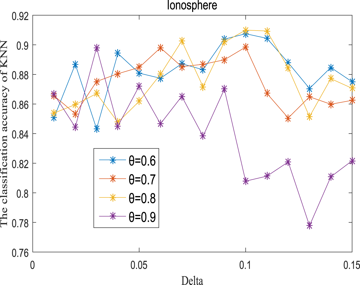
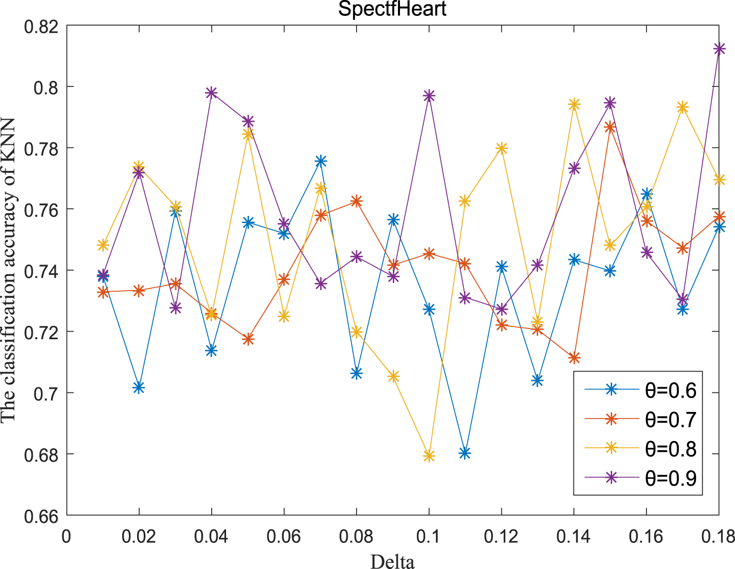
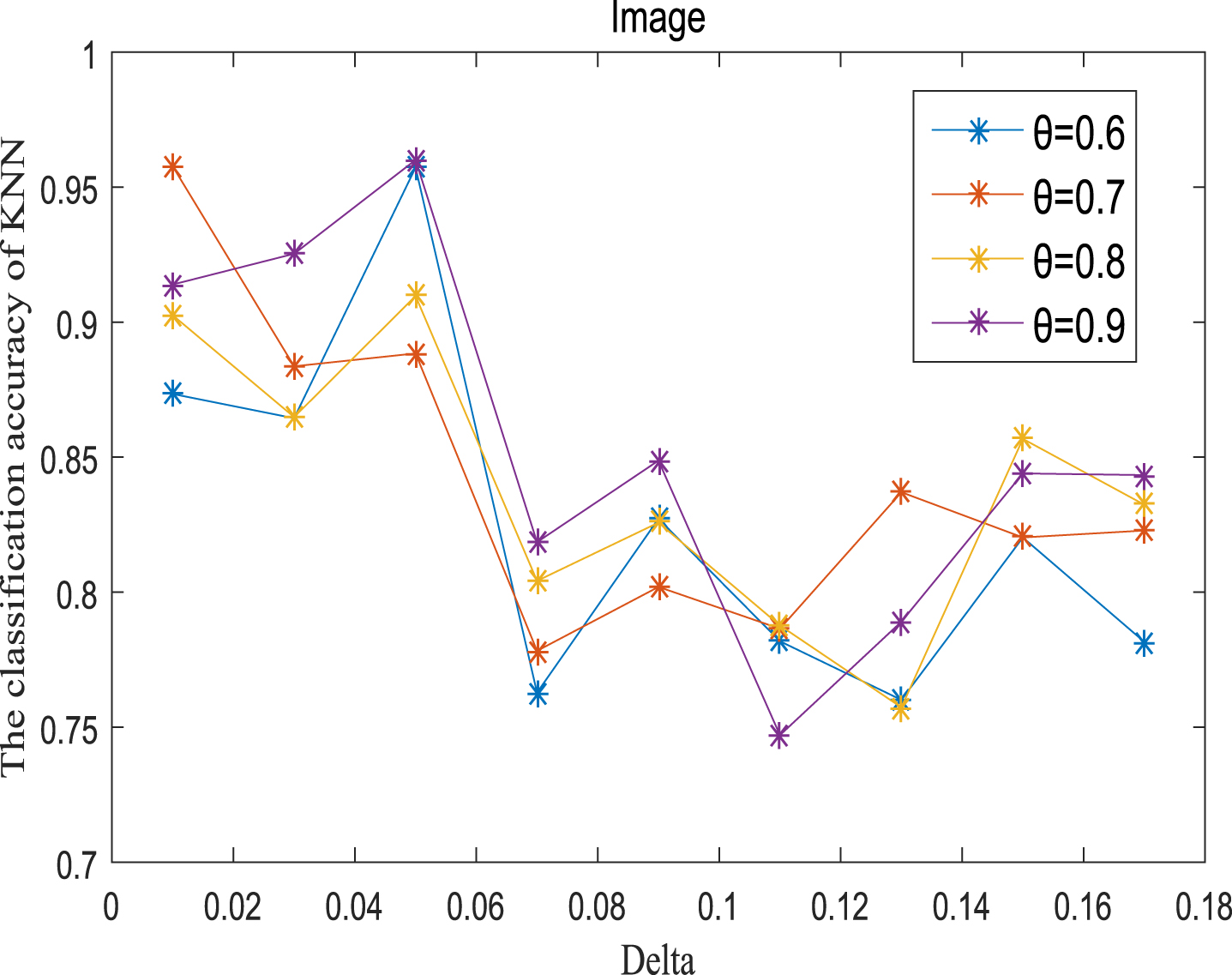
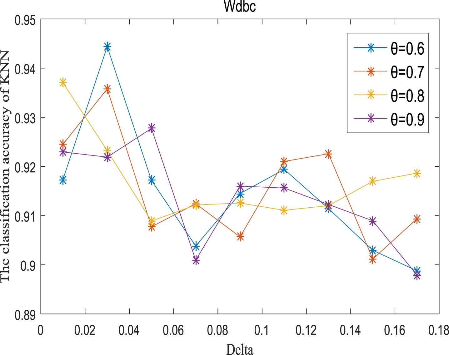
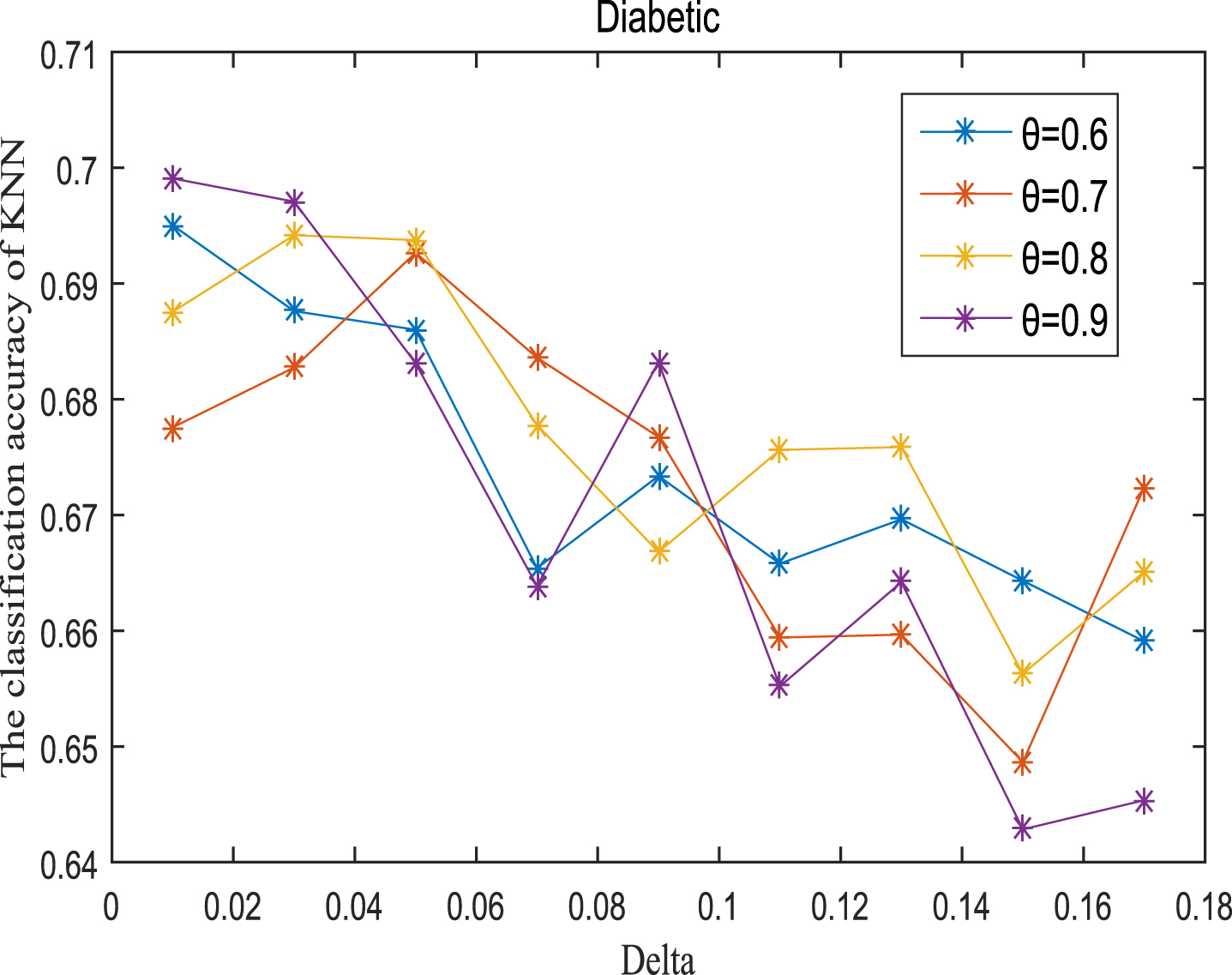
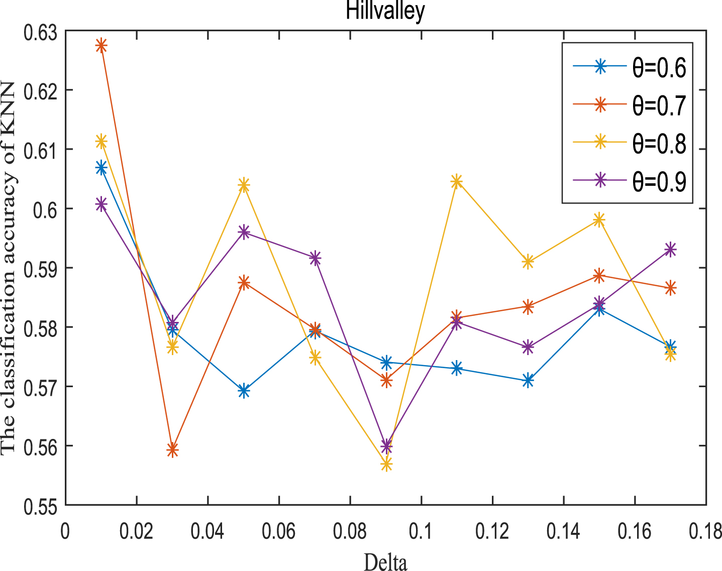
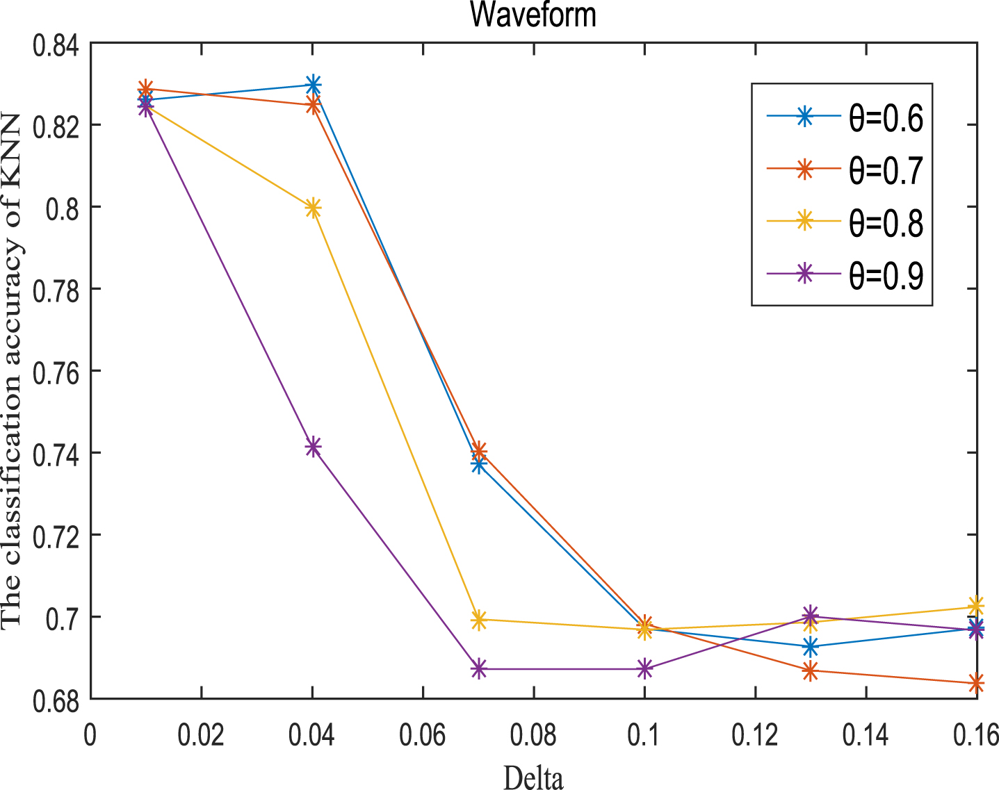
KNN classification accuracy (Wave).

OPEN IN VIEWER

Fig. 21

PNN classification accuracy (Fish).

OPEN IN VIEWER

Fig. 22

PNN classification accuracy (Car).

OPEN IN VIEWER

Fig. 23

PNN classification accuracy (Water).

OPEN IN VIEWER

Fig. 24

PNN classification accuracy (Ion).

OPEN IN VIEWER

Fig. 25

PNN classification accuracy (SH).

OPEN IN VIEWER

Fig. 26

PNN classification accuracy (IS).

OPEN IN VIEWER

Fig. 27

PNN classification accuracy (Wdbc).

OPEN IN VIEWER

Fig. 28

PNN classification accuracy (Dia).

OPEN IN VIEWER

Fig. 29

PNN classification accuracy (Hill).

OPEN IN VIEWER

Fig. 30

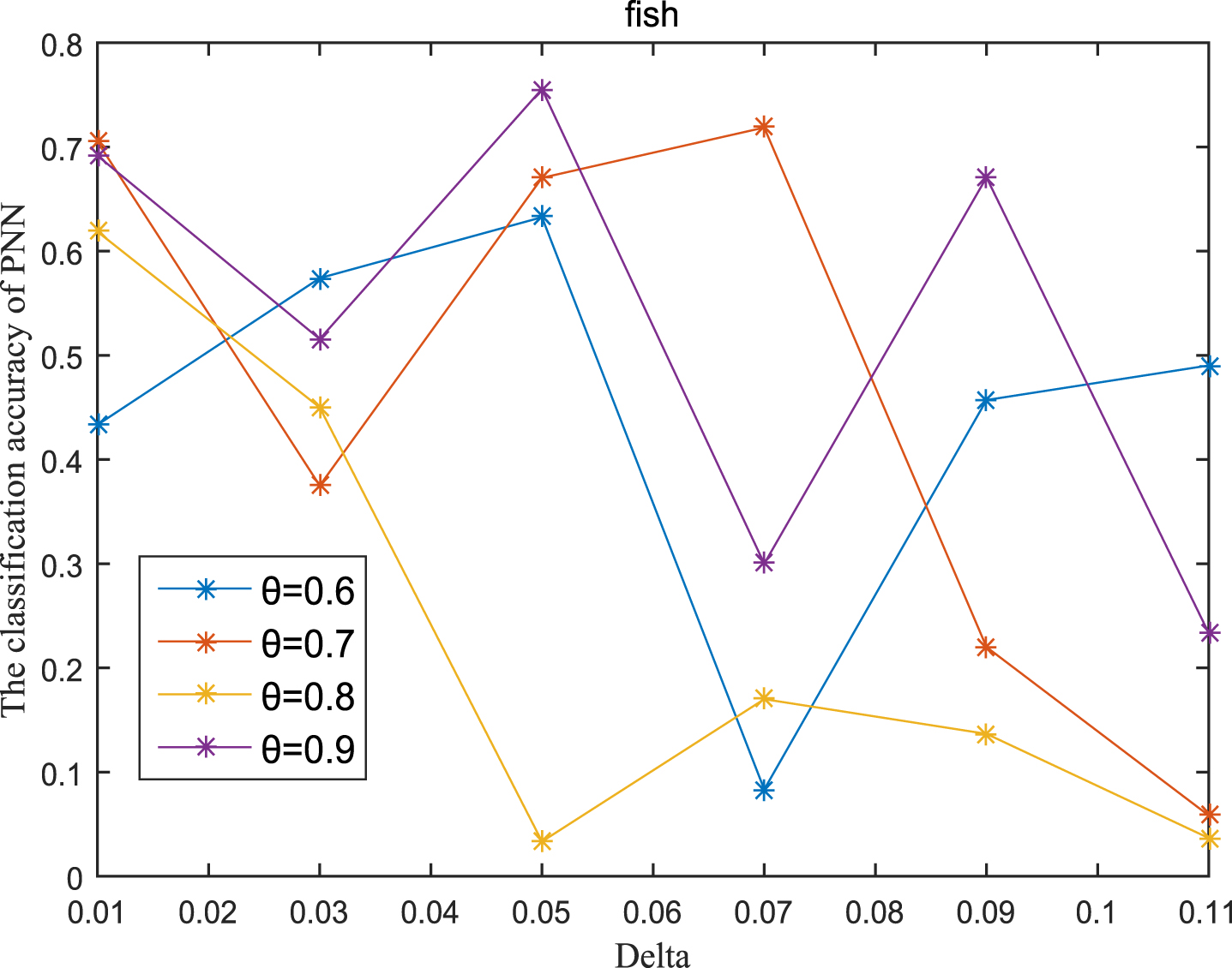
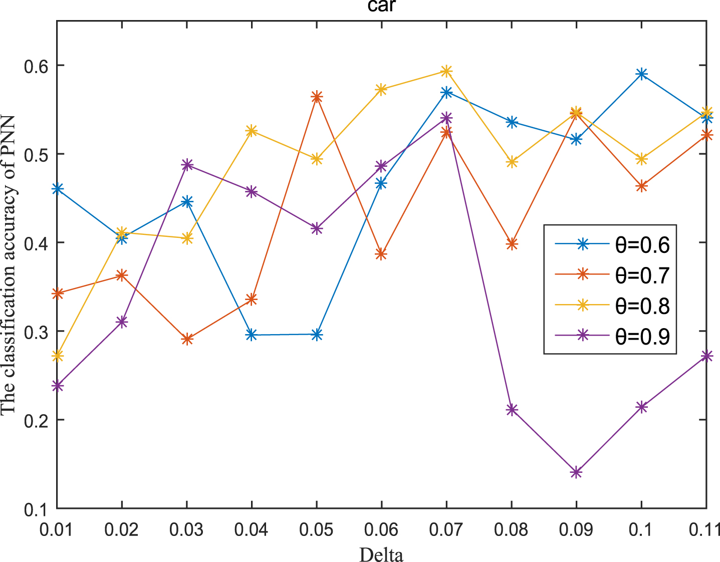
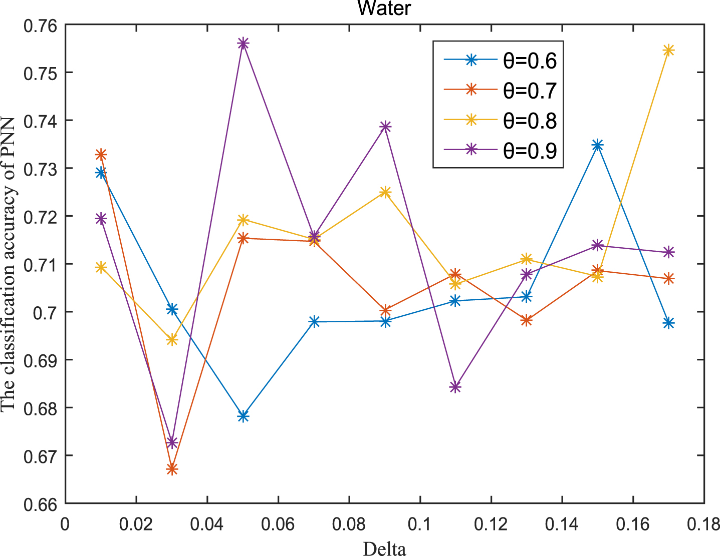
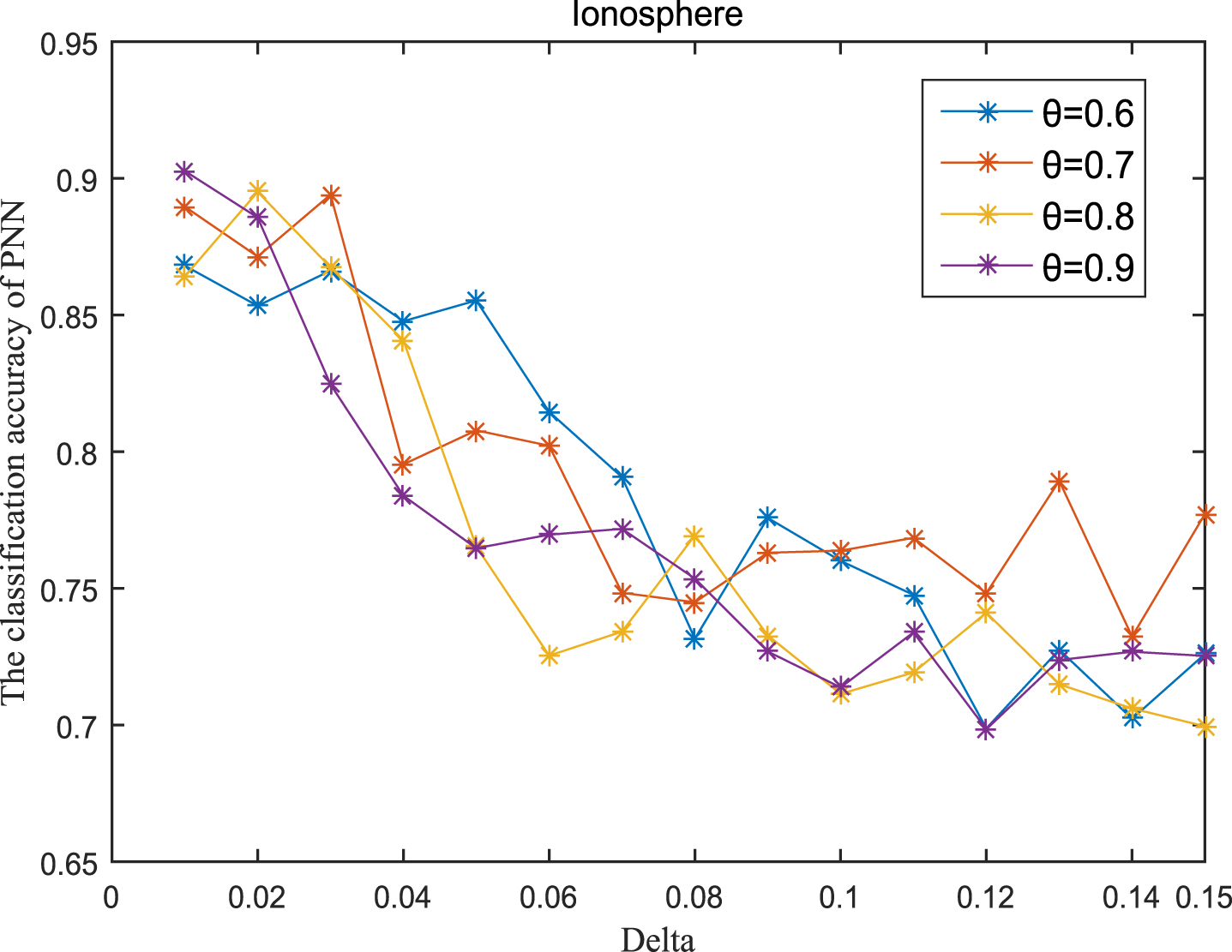
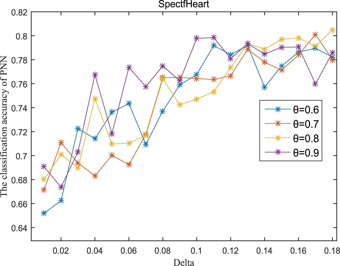
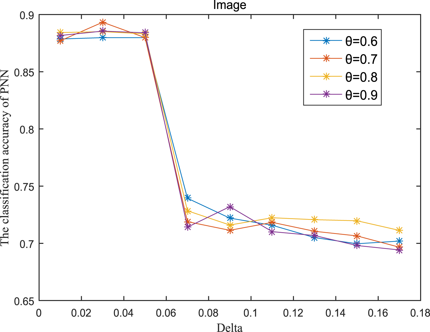
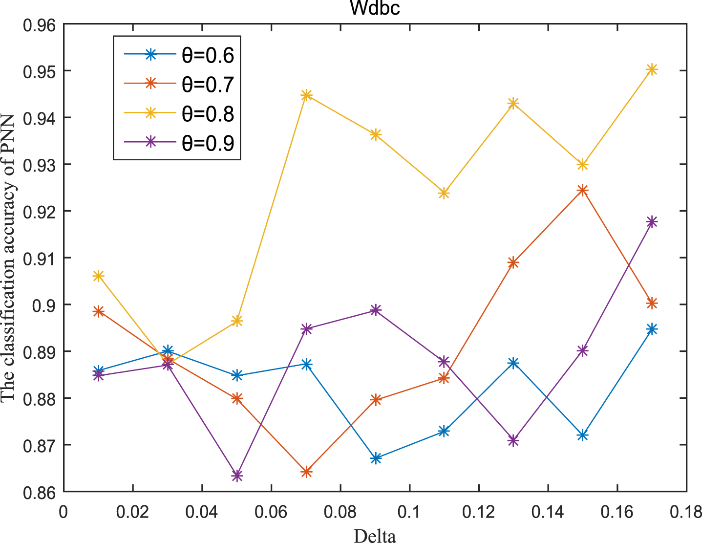
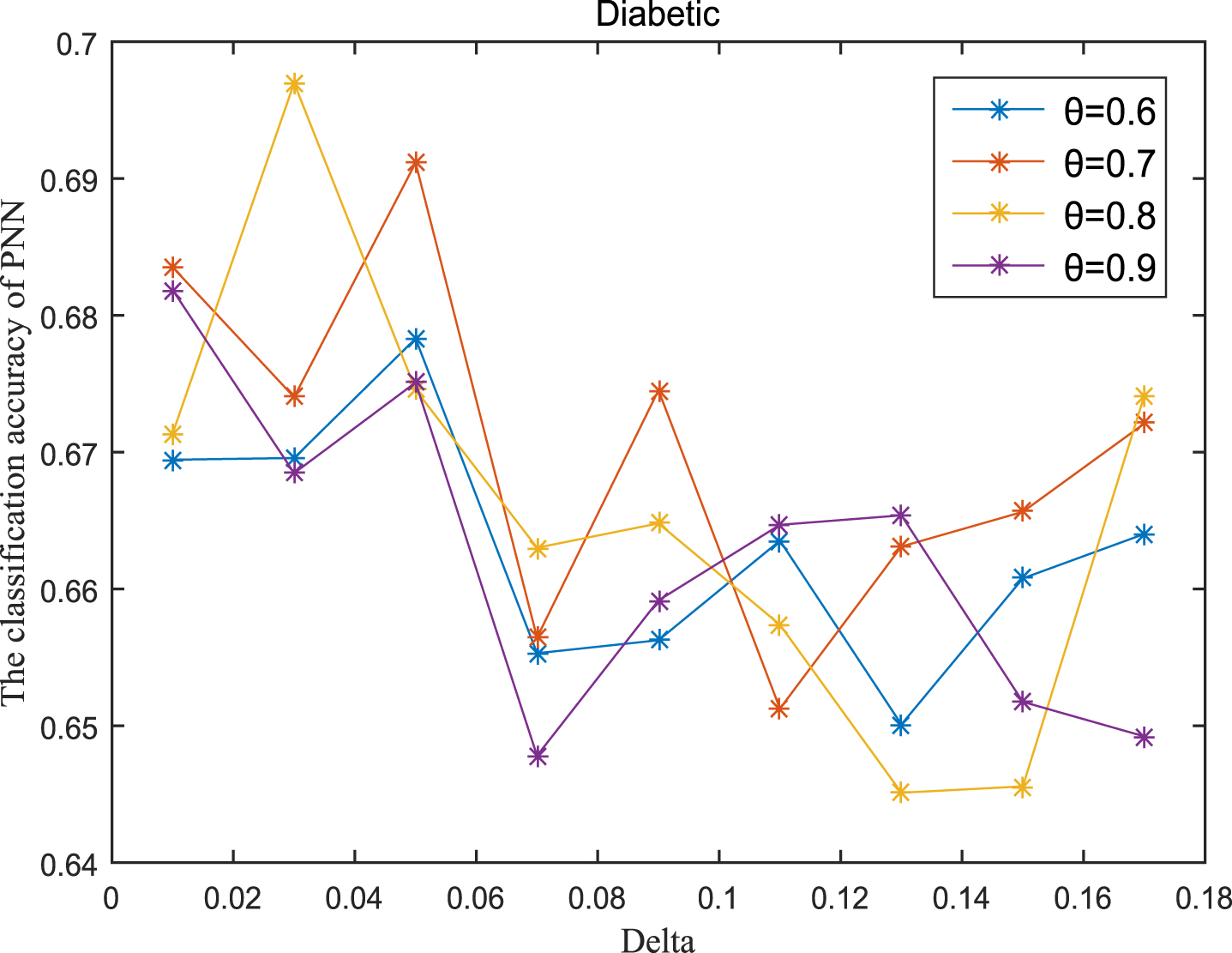
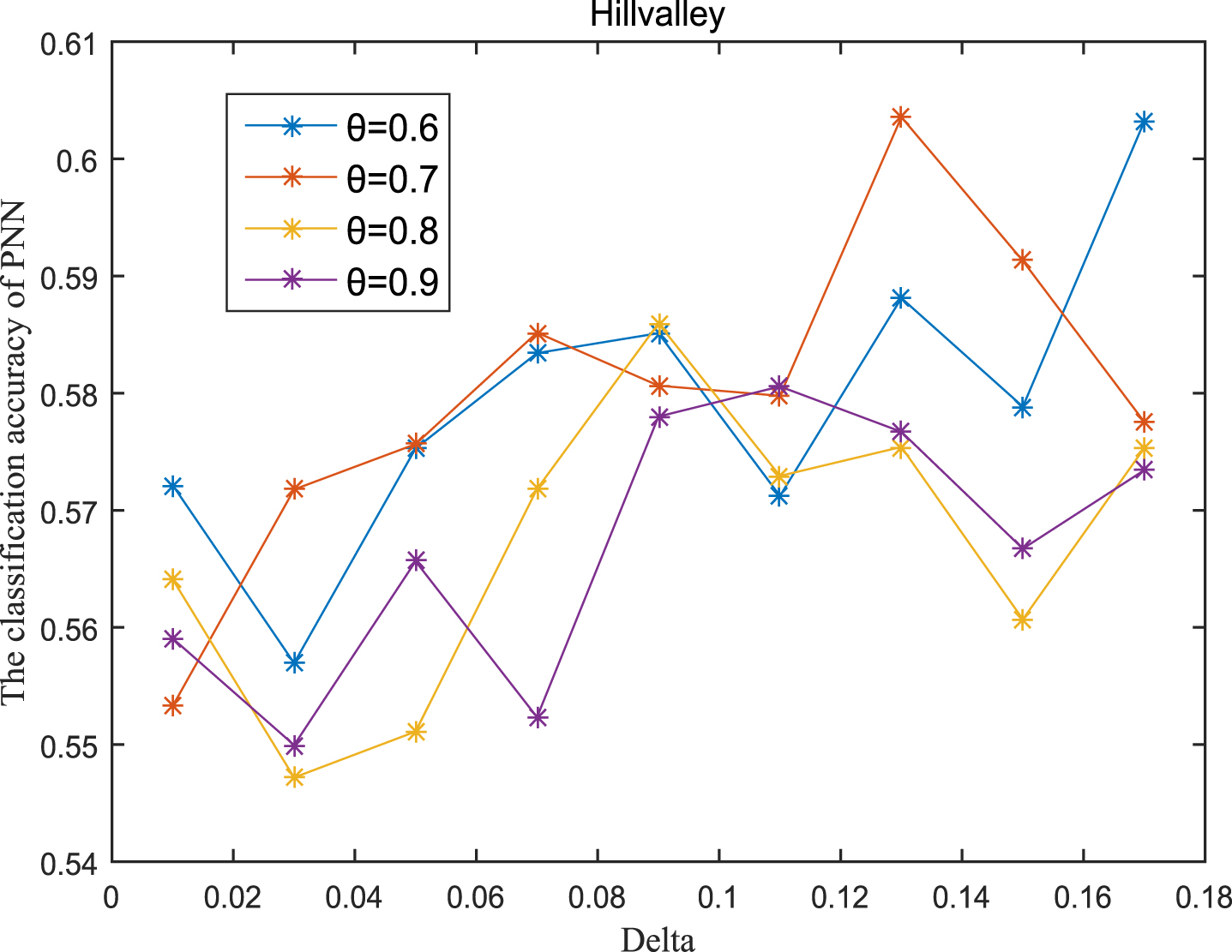
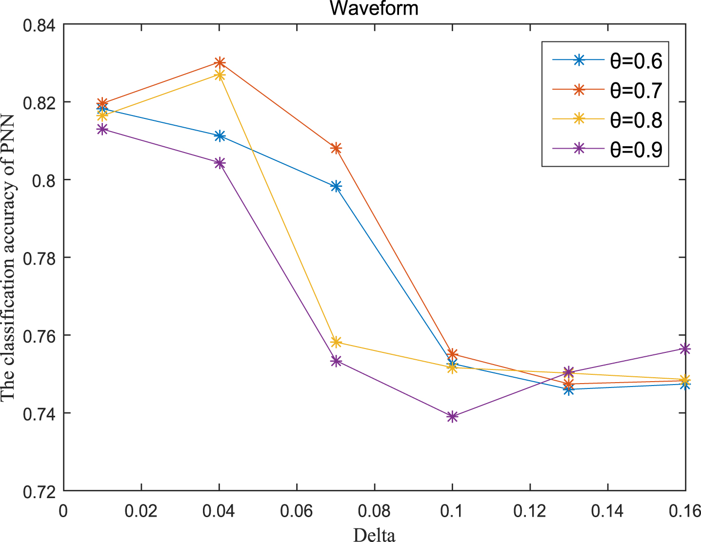
PNN classification accuracy (Wave).

In this section, we implement comparative analysis.

In order to show the advantages and disadvantages of the proposed algorithm, we choose the other five algorithms to compare with the proposed algorithm in this paper. One is PCA mentioned in the reference [33], whose contribution rate of characteristic root is assumed to be 0.95; one is FSRAR in the reference [23]; one is “DAI" in the reference [7]. The other two algorithms are COEN and DEP from the reference [3]. The computer used for the experiment is Lenovo PC, which is configured with Intel Core i7-4790cpu @ 3.60GHZ and 16G memory. The algorithm was programmed by Matlab 2015b. The four algorithms are tested with 10 datasets given in Table 2. Because the parameters selected by each algorithm are inconsistent, there will be multiple reduction sets calculated by one algorithm. We choose the set with the highest average classification accuracy as the reduction set. The classification accuracy is that each algorithm randomly selects 80% of the data as the sample, the remaining 20% of the data as the training set, runs 10 times and takes the average value.

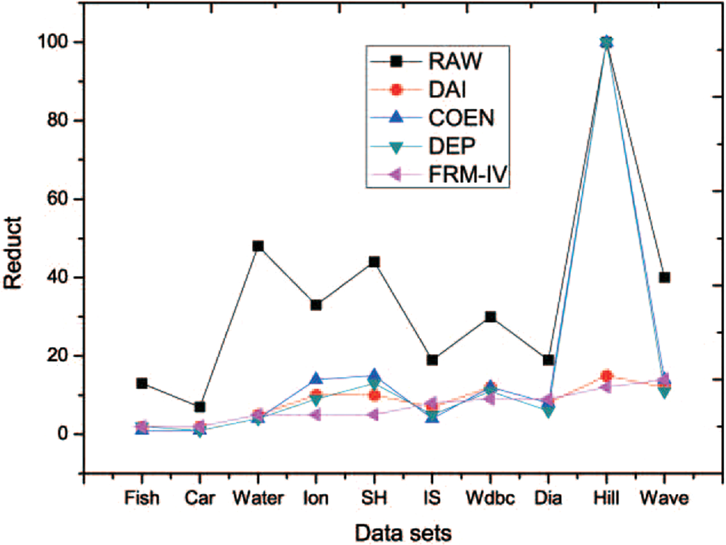
Table 3 shows the best reduction set under the maximum accuracy of the four algorithms. The ‘raw data’ list shows that the datasets has not been reduced. It can be seen from Table 3 that Hillville dataset has not been reduced under COEN. The reason is that the data set must be α-consistent, but α cannot satisfy the conditions from 0.1 to 0.99, so the algorithms have no effect on the dataset. The reduction effect of DEP and FRM-IV algorithm is the best, and the average set size is 7.1. Figure 31 graphically shows the reduction effects of various algorithms under 10 datasets.

OPEN IN VIEWER

Fig. 31

Reduced set comparison.

Table 4 shows the classification accuracy obtained by calculating 10 datasets with KNN classifier, where k = 3. Underlined values indicate the highest accuracy. It can be seen that FRM-IV algorithm does not perform well on fish and car datasets, but shows high accuracy on other eight datasets. Figure 32 shows the KNN classification accuracy curve on 10 datasets. The horizontal axis represents 10 datasets, and the vertical axis represents the classification accuracy. Through figure 32, we can more intuitively see that the data set reduced by algorithm FRM-IV is significantly better than the other three algorithms in classification accuracy.

OPEN IN VIEWER

Fig. 32

Comparison of classification accuracy (KNN).

Table 5 shows the accuracy of the reduced datasets classified by PNN classifier. It can also be seen that FRM-IV algorithm is not good enough in fish and car datasets, and the classification accuracy is not as good as the other three algorithms. However, the algorithm achieves high classification accuracy on the other eight datasets. Figure 33 is a visual display of data in Table 5. In general, the proposed algorithm can reduce the number of attributes and obtain better classification accuracy than the other three algorithms.

OPEN IN VIEWER

Fig. 33

Comparison of classification accuracy (PNN).

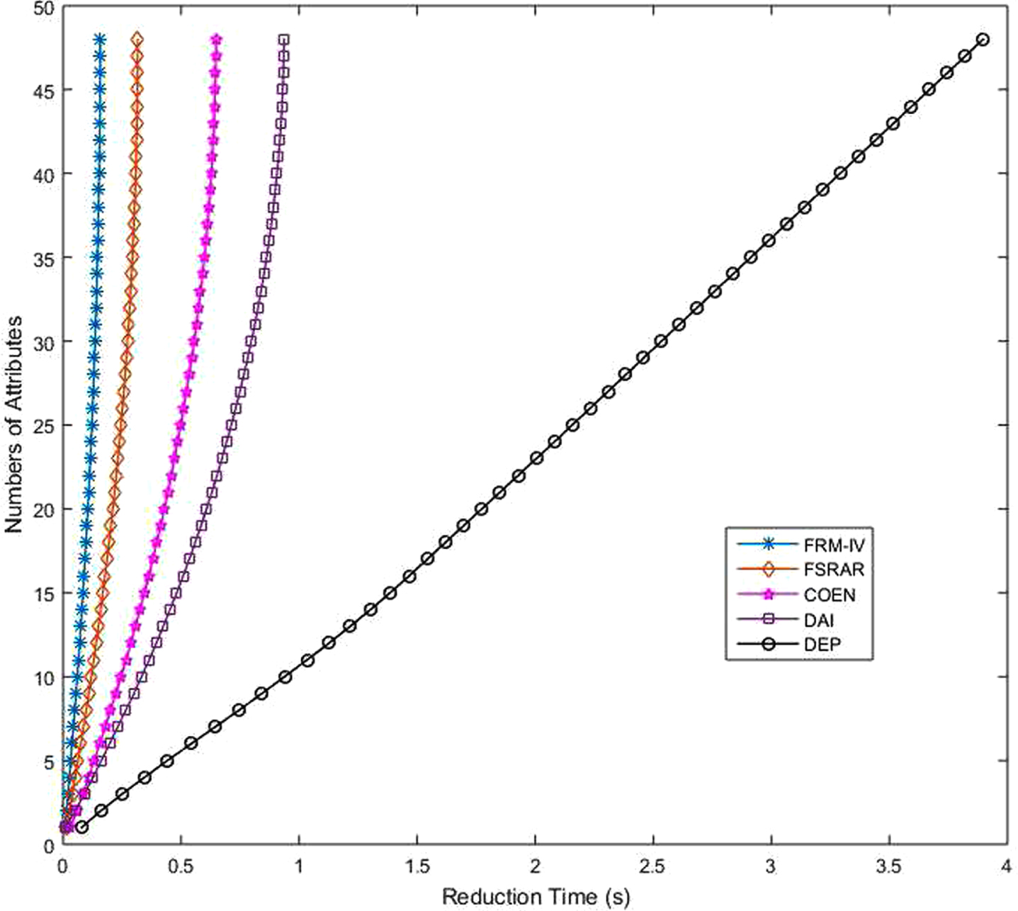
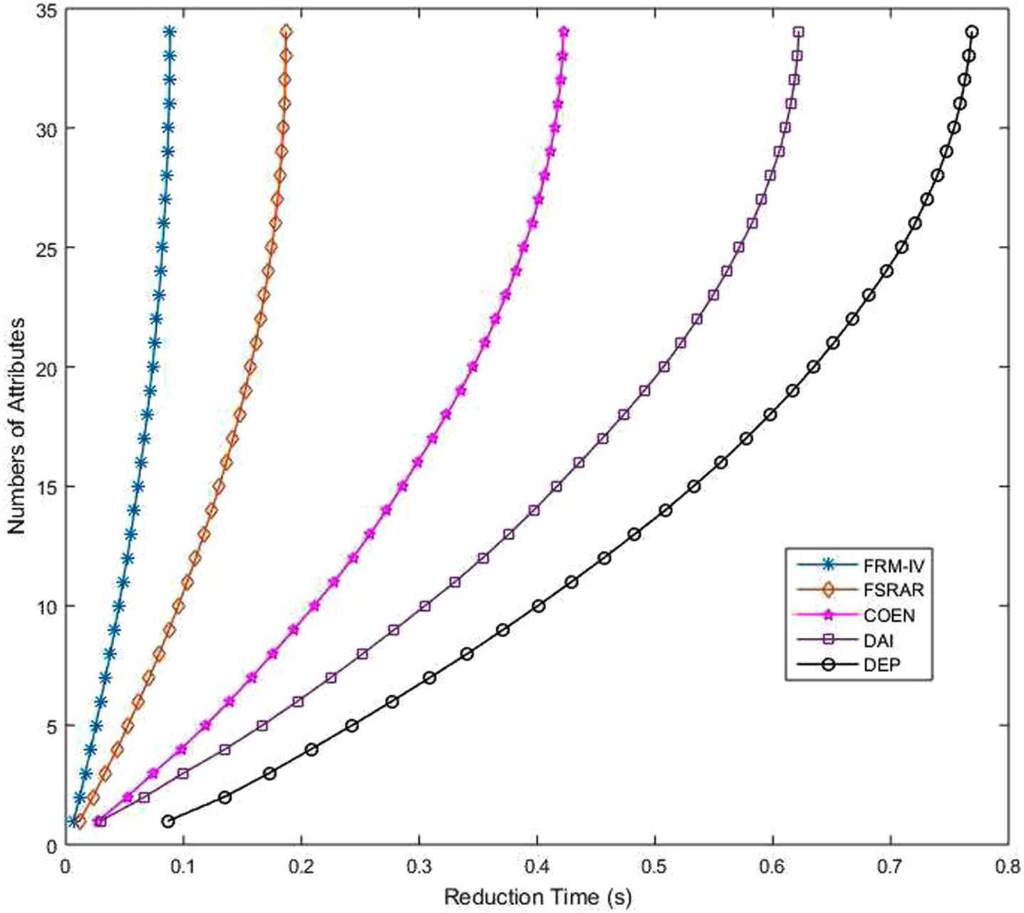
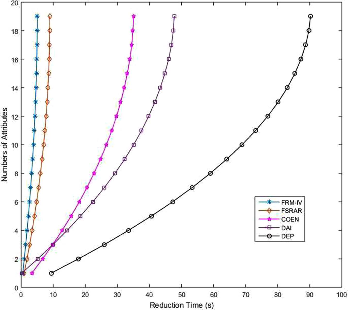
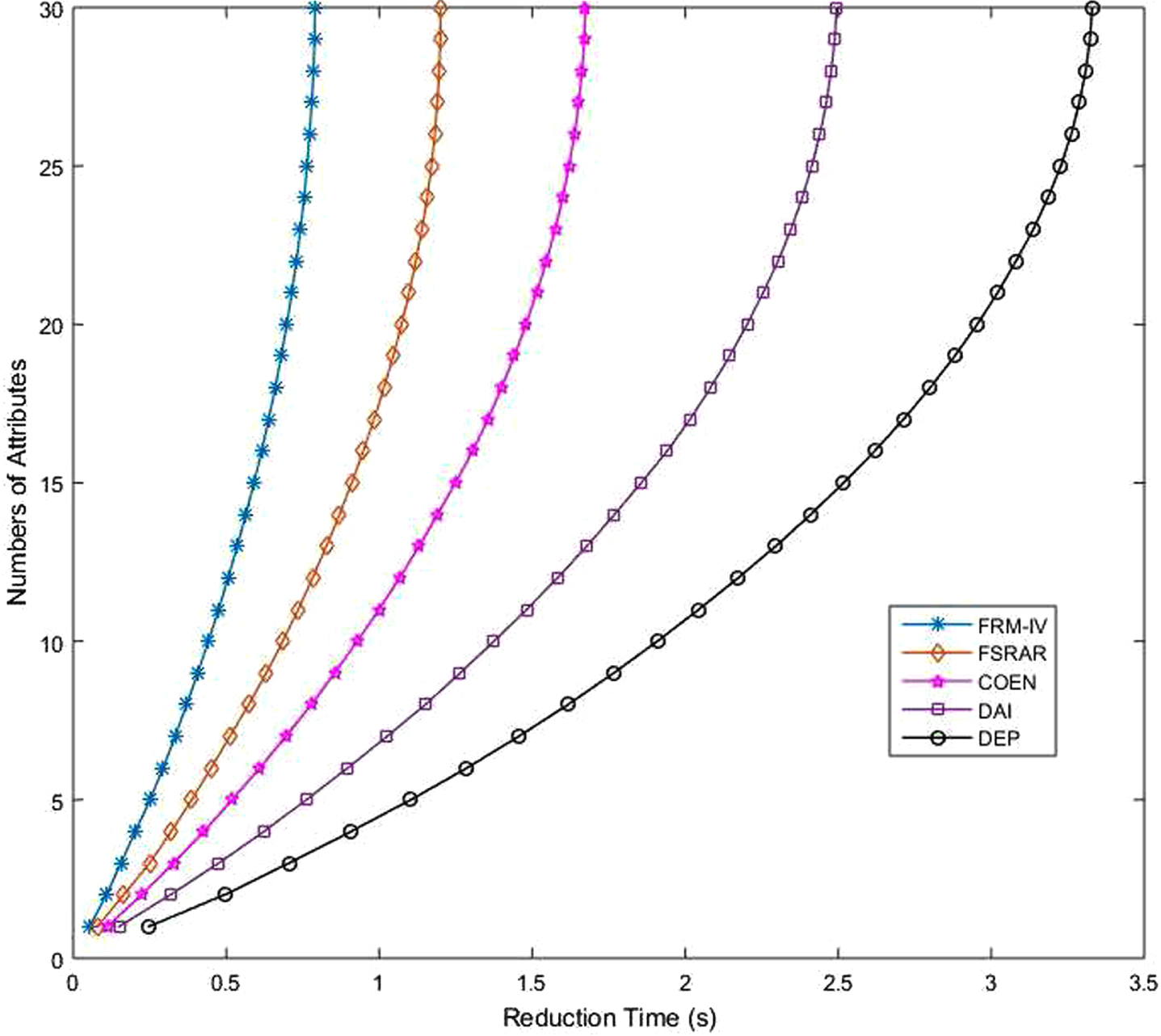
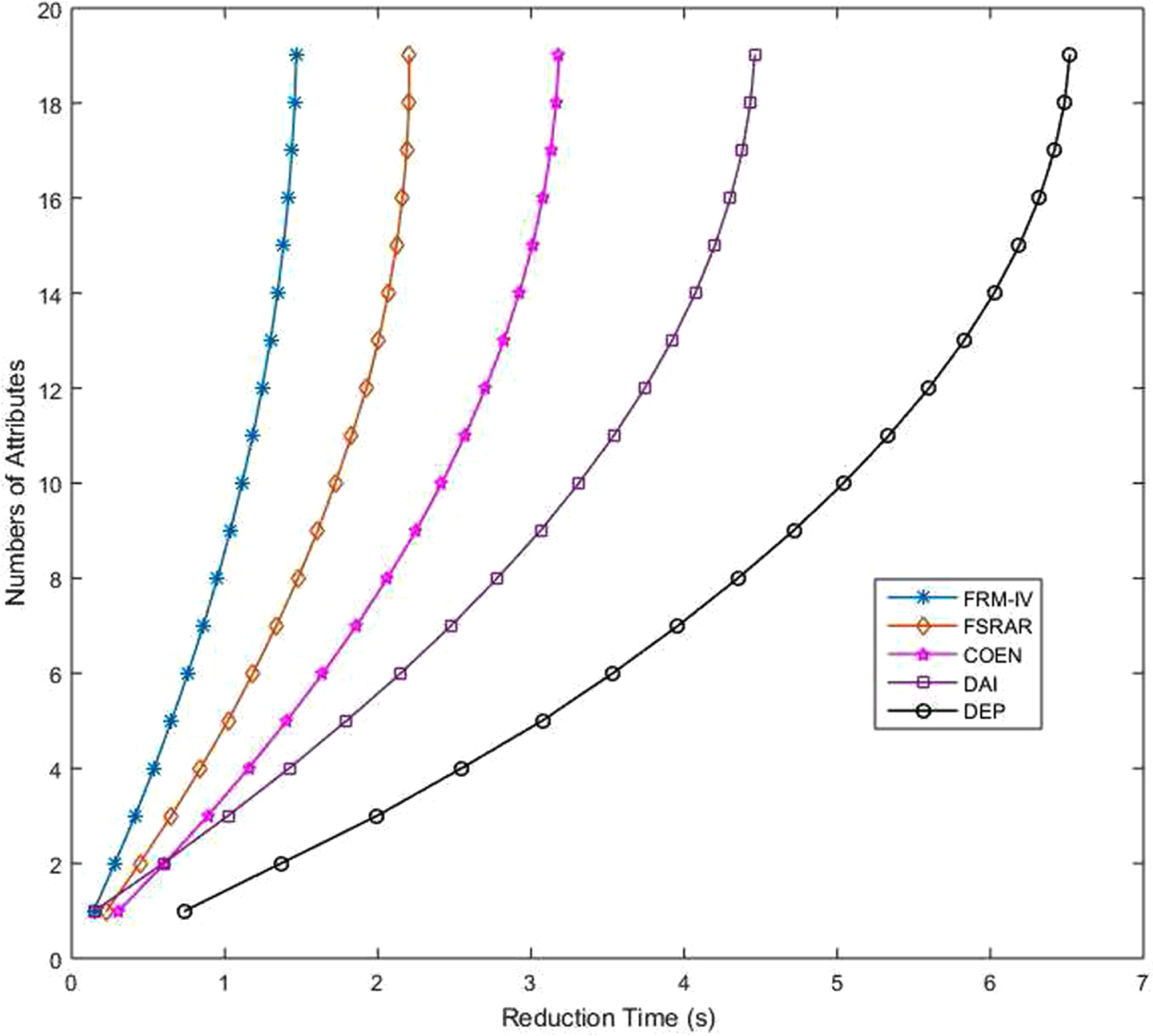
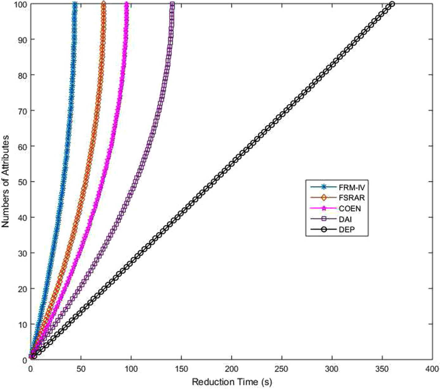
In addition to the comparison of algorithm accuracy, the reduction speed of several algorithms is also compared. Because PCA algorithm is the dimensionality reduction of data and does not involve feature selection, it does not compare the time consumption. In this work, the time consumption of five algorithms is compared. Adjust the termination conditions so that the algorithms will not stop until all attributes in the set are reduced. All algorithms start from the time of reduction. Figures 34-41 shows the time consumption comparison of five algorithms under different datasets. It is easy to see from the figure that the algorithm FRM-IV proposed in this paper is faster than the other four algorithms. It takes less time to reduce all attributes. The second fastest is FSRAR, the third fastest is COEN and the slowest is DEP. When a dataset with a large number of attributes is encountered, such as Water, Hill and Wave, DEP algorithm does not perform well, and the time consumption curve shows a straight line trend. In general, algorithm FRM-IV in this paper is better than other algorithms in terms of reduction set size, classification accuracy and operation speed.

OPEN IN VIEWER

Fig. 34

Time consuming comparison (Water).

OPEN IN VIEWER

Fig. 35

Time consuming comparison (IS).

OPEN IN VIEWER

Fig. 36

Time consuming comparison (SH).

OPEN IN VIEWER

Fig. 37

Time consuming comparison (IS).

OPEN IN VIEWER

Fig. 38

Time consuming comparison (Wdbc).

OPEN IN VIEWER

Fig. 39

Time consuming comparison (Dia).

OPEN IN VIEWER

Fig. 40

Time consuming comparison (Hill).

OPEN IN VIEWER

Fig. 41

Time consuming comparison (Wave).

In this section, Friedman test and its post-hoc test should be performed for illustrating the differences of classification accuracies among the proposed algorithms statistically.

Friedman test [10, 32] is an non-parametric test basing on the following basic ideas: firstly, the algorithms are sorted in ascending order by their comparing index values, and the ranks of each algorithm under different datasets are obtained; secondly, calculating the average ranks of different algorithms respectively and the average rank differences between each pairs of algorithms; at last, comparing the average rank differences with a corresponding critical value of the test.

The specific inspection process is as follows. In a test of m datasets and n algorithms, it ranks the n algorithms by their classification accuracies respectively. For the i-th data set, the algorithm with the highest classification accuracy ranks 1st, the algorithm with the second highest classification accuracy ranks 2nd, and the algorithm with the third highest classification accuracy ranks 3rd,⋯. If the two algorithms have the same classification accuracy, their ranks are averaged. Denoting the rank of the classification accuracy of the j-th algorithm under the i-th data set as a _ij , then the average rank of the j-th algorithm can be calculated as a j = 1 m ∑ i = 1 m a ij . The significance of the difference can be tested by the statistic F = ( m - 1 ) χ 2 m ( n - 1 ) - χ 2(29) where χ 2 = 12 m n ( n + 1 ) ∑ j = 1 n a j 2 - 3 m ( n + 1 ) . The statistic F is Fisher distributed with n - 1 and (m - 1)(n - 1) degrees of freedom. If the statistic value of F is bigger than the critical value of F _α(n - 1, (m - 1)(n - 1)) which depends on F(n - 1, (m - 1)(n - 1)) distribution and the given significance levels α, it indicates there are differences among the algorithms. This means a post-hoc test, such as Nemenyi test, is needed. Nemenyi test can be used to compare all classification algorithms against each other. It comes up with a critical distance CD _α, which can be denoted as CD α = q α n ( n + 1 ) 6 m(30) where q _α is a critical value of the Tukey distribution with n degrees of freedom. If the differences of the average ranks between two algorithms exceeds the critical distance CD _α, then the classification performances of the two algorithms are significantly different.

(1) Ranking the six algorithms by their classification accuracies on the ten datasets, respectively (see Tables 6 and 7).

(2) Conducting Friedman test. Under the six algorithms and the ten datasets, F follows the distribution F(5.45). Given the significance level α = 0.05, the critical value F _α(5.45) =2.422. χ² = 26.157, F = 9.873, F > F _α(5.45), this means the performance of the six algorithms are significantly different under the KNN and PNN classifier.

(3) To check out which algorithms perform better, a post-hoc test, that is Nemenyi test, is introduced. The results of Nemenyi test can be visually represented in Figure 42. The top line in the figure is the interval of CD _α, and the second line is the axis on which we plot the average ranks of different algorithms. The groups of algorithms that are not significantly different are connected by a horizontal line. Above all, the following results are obtained:

OPEN IN VIEWER

Fig. 42

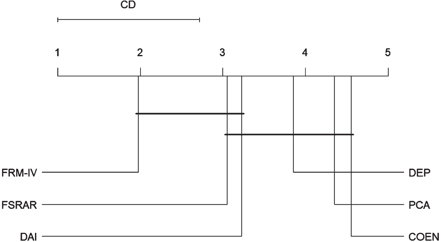
The Nemenyi test result with KNN and PNN.

a) The classification accuracy of FRM-IV is significantly higher than that of PCA, COEN and DEP;

b)The classification accuracy of FSRAR is significantly higher than that of PCA, COEN and DEP;

c)The classification accuracy of DAI is significantly higher than that of PCA, COEN and DEP;

d) There is no significant difference between the classification accuracy of FRM-IV, FSRAR and DAI;

e) There is no significant difference between the classification accuracy of PCA, COEN and DEP.

In this paper, some attribute evaluation functions that express the classification ability of feature selection have been put forward. Based on these functions, FRIC-model in an IVDIS has been established. An feature selection algorithm in an IVDIS has been presented by using this model. Experiments have been carried out and statistical tests have been used to evaluate the performance of the presented algorithm. Experimental results explain that the presented algorithm is more effective than some existing algorithms, and does not occupy too much memory. In the future, we will consider the application of FRIC-model.