
Abstract
This paper discusses an uncertain time optimal control problem by considering time efficiency, which is to optimize the objective function about the first hitting time subject to uncertain differential equations. According to the definition of the α-path, the uncertain time optimal control problem is transformed into an equivalent deterministic optimal control problem. Two kinds of time optimal control models are presented where optimistic value and reaching index are chosen as the optimality criteria, respectively. Applying the proposed uncertain optimal control model to a portfolio selection problem, we obtain the uncertainty distribution of the first hitting time (the investors’ first profit time). Meanwhile, sufficient conditions of the optimal control strategy of such models are provided. Numerical simulations are provided which reveal the change for our optimal control strategy.
Keywords
Introduction
Optimal control problem, which essential is a branch of modern control theory, has been developed rapidly since 1950s’. Pontryagin [26] pioneered the maximum principle which has been absorbed into the optimal control theory. Almost simultaneously, Bellman [27] proposed another mathematical method, dynamic programming, to handle optimal control problem. Besides, Kalman [28] presented kalman’s filtering to solve optimal control problem. Based on the contributions and attentions this field, optimal control theory has made great progress. Meanwhile, the application of optimal control theory involves many fields, such as power system, traffic system, manufacturing system and space technology, among others.
The control system is often disturbed by uncertain factors in different forms due to the uncertainty of the real world. Among them, stochastic disturbance is a kind of uncertainty which behaves randomness. Wonham [29] initially investigated the stochastic linear quadratic (LQ) optimal control problem. Then, scholars made a great deal of further researches on this field following the previous studies. Cairns [3] and Karatzas [6] studied optimal control problem of Brownian motion, which was applied to engineering as well as finance. Merton [23], Solow [35] investigated the stochastic optimal control model about the economic growth. For more details about stochastic optimal control, see references [30, 31] and [32].
Different from the classical optimal model to optimize expected utility over an infinite time horizon, this paper focuses on a time optimal control system, which studies the first hitting time of the objective function. It aims at seeking the optimal control such that a practical performance criterion about time under some constraints can be optimized. Since 1970s, researchers have studied stochastic optimal control for such problem. Ahmed and Teo [1] first proposed a kind of non-linear stochastic systems with controls which use only partial information about the current state. With Itô’s lemma, a time optimal control law of bang-bang control was shown and further be detained after solving a two-point boundary value problem involving systems of nonlinear integral-partial differential equations. In reference [19], a sufficient condition was presented for maximizing the probability that at a random time ω the state is in a given set. Zhu, Deng and Huang [21] investigated the optimal bounded control, which was governed by quasi-integrable Hamiltonian systems of wide-band random excitation, to minimize the so called first-passage failure. As for the first passage problem of non-stationary discrete-time control systems, reference [4] gave a so-called first passage optimality equation and proved the existence of optimal Markov policies.
The probability theory is known as an essential mathematical tool to handle the stochastic problem. However, if the data size is too small or the extreme case without data, probability theory may perform badly or even fail. In these situations, many professional experts are invited and their belief degrees are analyzed, which are used to measure the chances that the possible events are supposed to occur. To characterize personal belief degrees rationally, Liu [7] introduced the uncertainty theory for the first time which depicts the belief degree of uncertain event rationally. In 2009, Liu [10] polished it with defining uncertain measure axiomaticly. Meanwhile, uncertain differential equations (UDEs) were established by Liu [8] in 2008. In addition, by expounding the continuity of uncertain state variables and inverse uncertain distribution (IUD), Y-C formula [17] revealed the relation between the ordinary differential equations (ODEs) and UDEs. Equivalent to Hamilton-Jacobi-Bellman equation in the stochastic optimal control, Zhu [20] derived the optimality equation which is an important condition for solving the extreme value problem. Furthermore, another uncertain optimal control model was presented by Sheng and Zhu [14] in 2013, in which the critical value criterion is selected as the optimal value criterion of the model. Corresponding optimality equation was also given. In 2015, Yan and Zhu [16] discussed a bang-bang control model for uncertain switched systems. Shu and Zhu [15] considered an uncertain linear singular systems control with optimistic value criteria and its application. If readers want to continue reading researches about optimal control, you can go through [36–38].
In practice, uncertain factors may influence the normal operation of the system, and even cause the system to crash. Thus it is meaningful and necessary to include these uncertain factors into optimal control model. Liu [11] firstly presented the definition of the first hitting time under uncertain environment in 2013. Then, for the solution to UDEs, Yao [18] studied their first hitting time and corresponding uncertainty distributions. Thus, it is notable to study uncertain optimal control model with the first hitting time. Inspired by Zhu’s [20] preceding works, we propose a time optimal control system from another perspective, where the objective function is involved with the first hitting time. In addition, we discuss a portfolio selection problem and a first-order circuit problem as the application of the proposed model, and use the optimistic value and reaching index as the optimality criterion, respectively. To the best of our knowledge, there has no study about such model. In addition, there are many studies on parameter estimation in uncertainty theory. Yao [39] proposed the method of moment to estimate the parameters of uncertain differential equations. Based on the difference form of uncertain differential equations, it was proved that the function of parameters obeyed the standard positive uncertainty distribution. Liu [40] presents a method of moments based on residuals to estimate the unknown parameters in uncertain differential Equations. A stock price example is used to illustrate the method.
Portfolio optimization has always been a very important problem in the financial market. It focuses on how to choose the optimal portfolio strategy to maximize the investment return and minimize the investment risk. Markowitz [41] is the first scholar to study this kind of problem. He introduced variance to quantify investment risk. Nowadays, a lot of portfolio model combined with uncertainty theory in the paper. Qin [42] proposed the uncertain mean-semi-absolute deviation model and transformed the proposed model into an equivalent deterministic form using the uncertainty distribution of security returns. Li [43] proposed a mean-variance-entropy model for the uncertain portfolio optimization problem, which used entropy to measure the diversification degree of the portfolio, and realized the maximum return and minimum risk in the form of a single objective, and verified the effectiveness and practicability of the model. For more details about portfolio selection, see references [44, 45] and [46].
The organization of this paper is as follows. In section 2, we review some basic definitions and theorems of the uncertainty theory. The time uncertain optimal control problem is modeled and converted into a corresponding crisp optimal problem in Section3. Two novel time optimal control models are presented where optimistic value and reaching index are chosen as the optimality criterion, respectively. In section4, a portfolio selection model is given, sufficient conditions for optimal control strategy of first hitting time about optimistic value-based model and reaching index model are given and numerical simulations are also obtained, respectively. In addition, the trend of the optimal control strategy is given in this section. Finally, the conclusions are summarized in section5.
Preliminary
For convenience, in this section, we recall some fundamental notations and useful concepts about the uncertainty theory such as uncertain measure, optimistic value, first hitting time, UDE’s α-path. Refer to [8–10] to know more information about the uncertain theory.
C0 = 0, at the same time nearly all sample paths are Lipschitz continuous; C
t
has stationary and independent increments; Every increment Ct+s - C
s
is a normal uncertain variable with expected value 0 and variance t2, i.e,
Then, UDE was proposed by Liu in 2008 as a type of differential equation governed by a canonical Liu process.
An uncertain process is a mathematical method to characterize human uncertainty provided by an uncertain differential equation. The general uncertain optimal control is widely known to find the best decision u t to optimize the total assets in infinite time domain. Nevertheless, time efficiency is essentially another important and meaningful factor in uncertain optimal control model. First hitting time is the first type of indeterminate time entered comed into our sight. For example, decision makers want to reach the ideal threshold (profit state) for the first time, the sooner the better. Furthermore, considering the special first hitting time of “failure”, decision makers often want to spend the least cost or the most efficient before the first hitting time. Based on such problem, uncertain optimal control problem with the first hitting time objective is essentially an optimal control problem of a kind of end value performance index, where the objective function is related to the first hitting time τ z that J (X t ) reaches z and the constraint is determined by a UDE.
Since τ z is an uncertain variable, the objective function cannot be considered as an ordinary function to be optimized. For the sake of ranking different uncertain variables or finding the largest one of them, different methods can be established with different optimality criteria, such as expected values, optimistic values, pessimistic values, and other uncertainty measures [22].
We propose the following uncertain control problem with the first hitting time objective function and an uncertain system
Now let’s transform the proposed uncertain optimal problem Ip to an equivalent deterministic optimal control problem.
Hence, we immediately have
Then, we propose the following two time uncertain optimal control problems and corresponding crisp problems, where optimistic value and reaching index are chosen as the optimality criteria, respectively.
VaR (Value at Risk), which is a quantitative measure about risk, refers to the maximum loss of a certain portfolio in a period under a certain probability. Based on the concept of VaR for loss function was introduced in 2013, Peng [24] first included uncertain factor into VaR. Then, Liu and Ralescu [25] discussed the corresponding VaR of uncertain random system.
In the real world, the first hitting time τ z that J (X t ) reaches z is greatly affected by uncertain factors. Therefore, it is difficult for us to use the expected value to rank the first hitting time τ z under different control strategies. Considering the VaR, optimistic value seems a better choice to measure the first hitting time τ z . That means, the bigger the optimistic value is, the bigger the first hitting time τ z is. Then, optimizing the first hitting time is equivalent to minimize its corresponding optimistic value. A first hitting time optimistic value-based model is given as below
According to Theorem 3.1, the optimistic value-based model is equivalent to the model
The proof is completed.
The first hitting time τ
z
that J (X
t
) reaches z in the optimal control model (3)is
Let’s introduce a reaching index
Therefore, a conservative decision maker need to maximize Rea in period [0, T], an uncertain first hitting time reaching index model is proposed as below
The theorem is proved.
In this section, the time optimal control model is applied to a portfolio selection problem with uncertain factors. Suppose that investors allocate their personal wealth. There are only two kinds of assets, one is the sure asset and the other is the risk asset. In stochastic environment, a portfolio selection model assumed that the risk asset brings a random return back, which was early studied by Merton [12, 23], and then generalized by Kao [5]. Zhu [20] considered the risk asset return as an uncertain variable in the generalized Merton’s model and a portfolio selection model of uncertain optimal control was provided, where the expected value was chosen as the optimality criterion. Sheng and Zhu [14] further studied an optimistic value model. However, when investors value the time efficiency, they prefer to minimize the first hitting time (first profit time) rather than maximize the expected utility. Here, such problem can be modeled by an uncertain time optimal problem.
In this model, we define the following notations. X
t
is the asset of an investor at time t, J (X
t
) is a utility function, w is the propotion allocated to the sure asset while 1 - w is that to the risk asset. The sure asset brings a earning rate b, and the risk asset brings an uncertain return which has a return mean rate μ (μ > b) and variance σ2. That means, in the time interval (t, t + dt), the risk asset earns a return dr
t
= μdt + σdC
t
, and the wealth level X
t
is modeled by a UDE
Let
For getting the optimal control strategy w∗ of the portfolio selection model, an important theorem about the uncertainty distribution U (s, w) of the first profit time τ z that J (X t ) reaches z is introduced as below.
Optimistic value-based model of portfolio selection is presented as follows
According to Theorem 3.2, it can be transformed into the following model
Now let’s move on to the sufficient condition of the existence of optimal control strategy w∗ in the portfolio selection problem (17).
According to Theorem 4.2, the optimal control strategy of the model (17)is the zero point of the function T (w), which would be calculated by the the algorithm as below.
1: Input a = 0, b = 1, ɛ > 0.
2: Let l = (a + b)/2.
3: If T (c) <0, l ← a. Otherwise, set l ← b.
4: If |b - a| > ɛ, go back to 2. Otherwise, output c as the optimal control strategy.
For different confidence level β, we first calculate corresponding zmin = exp(- bλ2/k2), which is the sufficient condition of the existence of optimal control strategy w∗.
Then, for z satisfying z > zmin in Table 1, we obtain the optimal investment proportion w* for different z and β by algorithm 1.
The minimum of z for different β.
Table 2 indicates that the optimal investment proportion w∗ reduces as the increasement of the given level z. In addition, for a fixed z, the bigger the confidence level β is, the lower the optimal investment proportion w∗ is. This trend of w∗ shows that if investment decision makers need to achieve the desired z as quickly as possible, or they have higher confidence level, they should allocate less in the sure asset and more in the risk asset.
Meanwhile, corresponding optimal value [τ
z
] sup(β) is provided. As shown in Fig. 1, for a larger z, the optimal optimistic value of the first profit time is larger (maximum
When other parameters are fixed, Table 3 indicates that the optimal investment proportion w∗ decreases as μ increased while increases as λ increases. Table 4 indicates that the optimal investment proportion w∗ decreased as σ increases while increases as b increases.
The optimal investment proportion w∗ for different λ and μ with z = 4, β = 0.6, b = 0.4, σ = 0.1.
The optimal investment proportion w∗ for different b and σ with z = 4, β = 0.6, λ = 0.2, μ = 0.6.
The corresponding optimal value [τ
z
] sup(β) with respect to different μ and λ is provided in
Fig. 2, which shows that for a relatively large μ,

Optimal objective value of different λ and μ with z = 4, β = 0.6, b = 0.4, σ = 0.1.
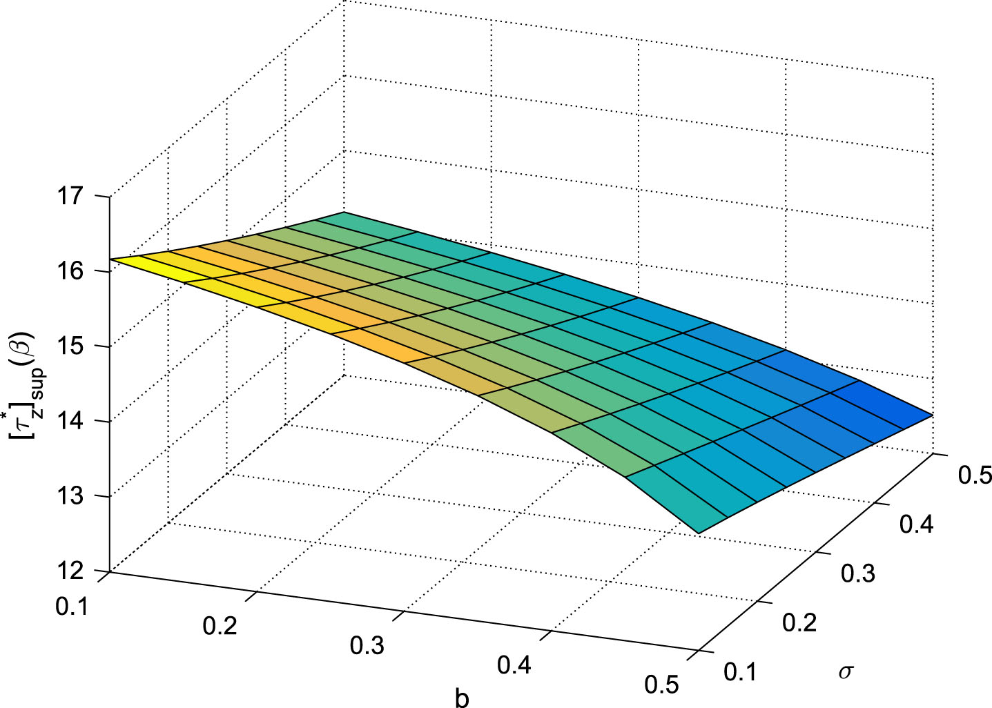
Optimal objective value of different b and σ with z = 4, β = 0.6, λ = 0.2, μ = 0.6.
Next we move on to measuring the sensitivity of our solution w to the parameter p by the relative change. The sensitivity is denoted as S (w, p)
According to Tables 2, 3 and 4, we obtain the sensitivity of different parameters as below.
The optimal investment proportion w∗ for different confidence level and pre-given level with λ = 0.2, μ = 0.6, b = 0.4, σ = 0.1.
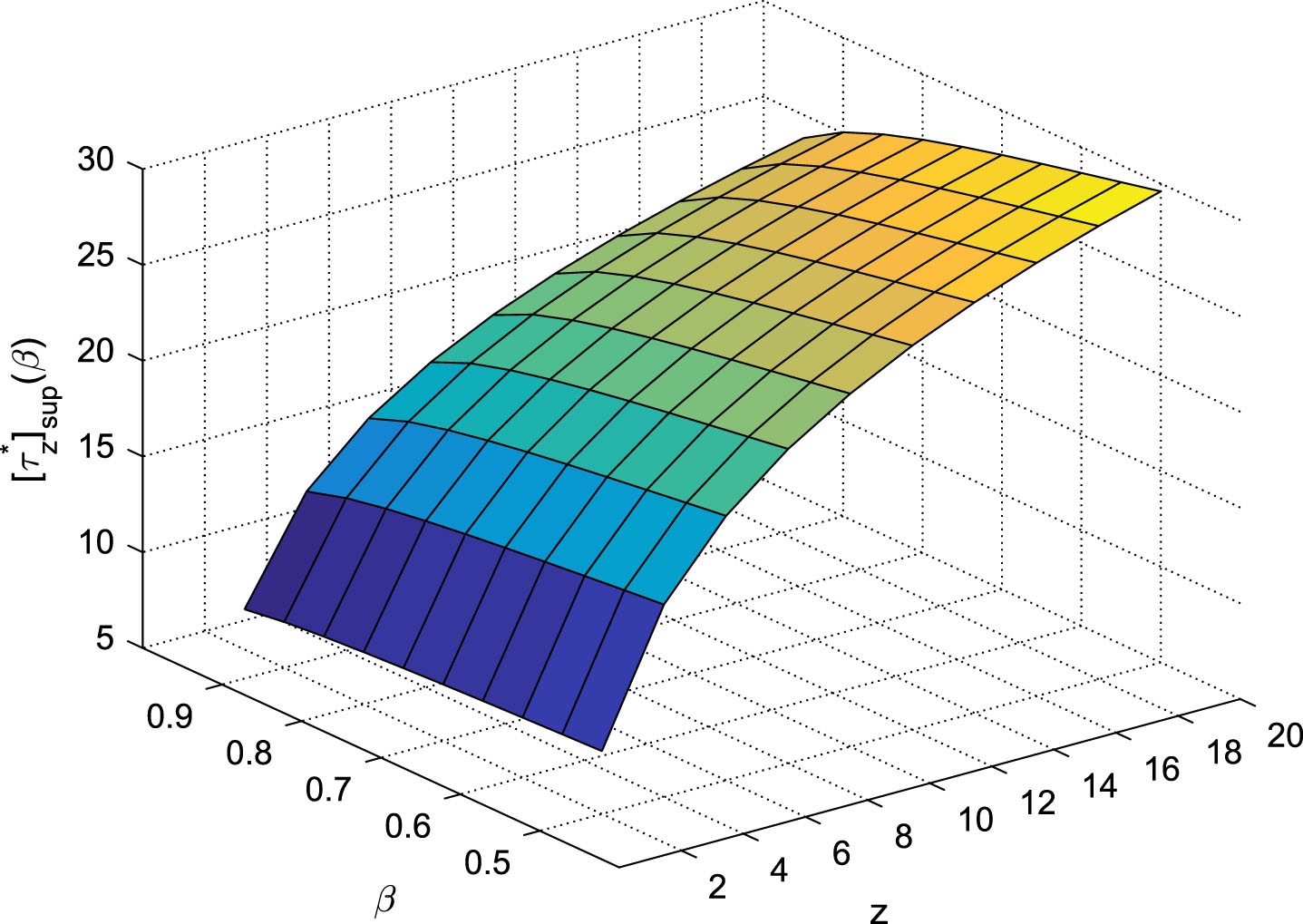
Optimal objective value of different confidence level and pre-given level with λ = 0.2, μ = 0.6, b = 0.4, σ = 0.1.
The sensitivity about different parameters.
Reaching index model of portfolio selection is presented as below
By Theorem 4.3, the optimal control strategy of the model (20)is the zero point of the function Q (w), which would be obtained by Algorithm 1.
For different given level z, we first calculate corresponding
The maximum of T of different z.
The optimal investment proportion w∗ of different pre-given level and maturity time with b = 0.4, σ = 2, λ = 0.5, μ = 2.
Table 7 indicates that the optimal investment proportion w∗ increases with the increase of the maturity time T. In addition, for a fixed T, the bigger the given level z is, the lower the optimal investment proportion w∗ is. The trend of w∗ demonstrates that when investors want to maximize the reaching index before a respectively large maturity time T, they should allocate more to the sure asset and less to the risk asset, while when they want to maximize the reaching index for a larger z, they should allocate less to the sure asset and more to the risk asset.
Optimal value of reaching index according to the optimal investment proportion w∗ is also shown in Fig. 4, which is in accordance with the actual situation that for a larger maturity time T, the corresponding optimal reaching index is larger (maximum Rea
Optimal objective value of different pre-given level and maturity time with b = 0.4, σ = 2, λ = 0.5, μ = 2.
When other parameters are fixed, Table 8 indicates that the optimal investment proportion w∗ increases as b and λ increase. Meanwhile, according to the optimal investment proportion w∗, the optimal value of reaching index is also shown in Fig. 5.
The optimal investment proportion w∗ of different b and λ with T = 10, σ = 2, z = 20, μ = 2.
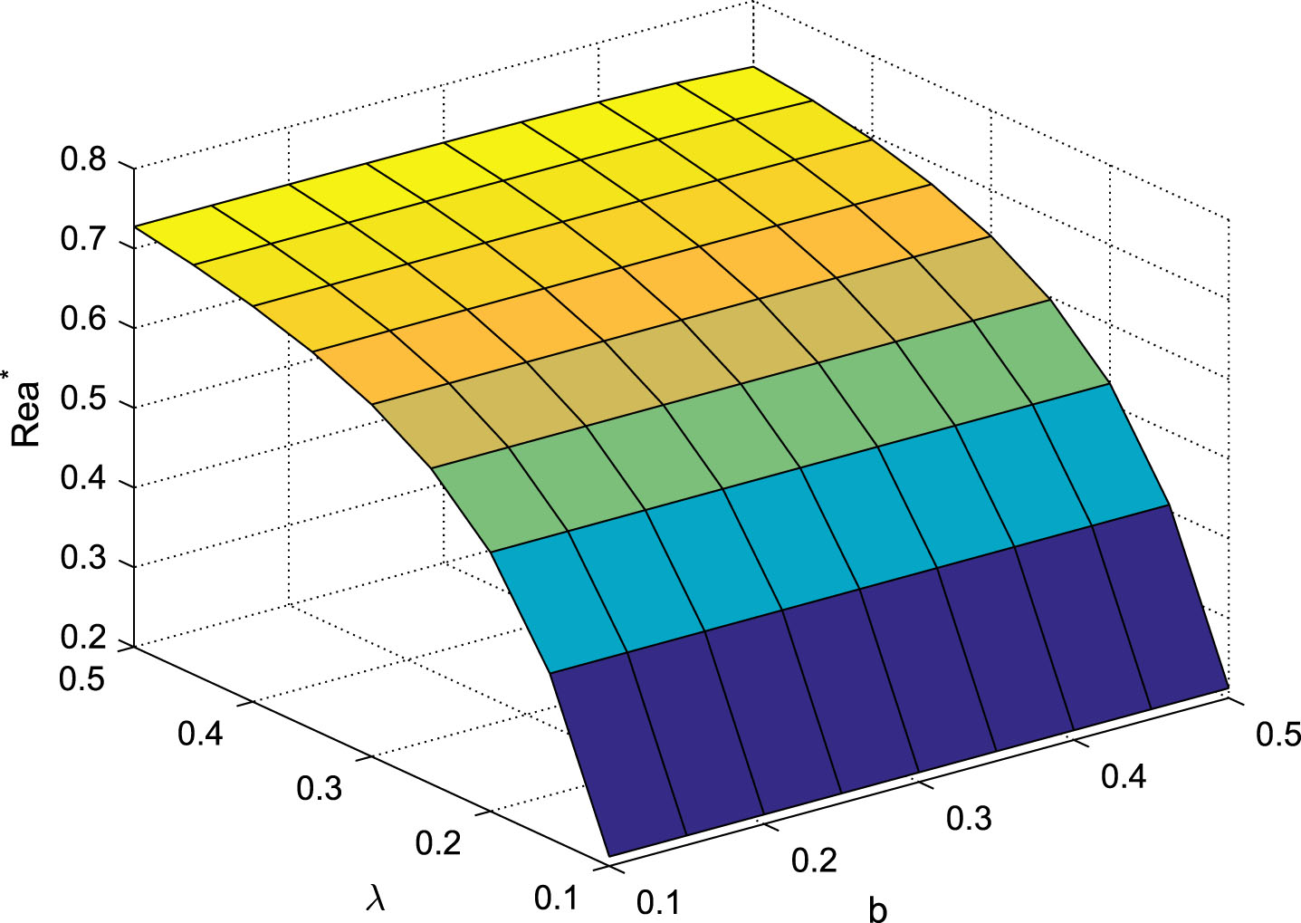
Optimal objective value of different b and λ with T = 10, σ = 2, z = 20, μ = 2.
By Tables 7 and 8, we obtain the sensitivity of different parameters as below.
The sensitivity of different parameters
Reaching the optimal time also brings meaning to the uncertain optimal control model. As a counterpart of uncertain optimal control system with the expected utility objective function, an uncertain optimal control model with the first hitting time objective was introduced, where the objective function is related to the first hitting time. Two special time optimal control models considering optimistic value, reaching index respectively as optimality criteria were thus presented. As an application, a portfolio selection model was provided to optimize the first profit time in uncertain environment. Explicit expression of the uncertainty distribution of the first profit time were given, based on which, optimal control strategy w∗ of such two models were obtained by the bisection method numerically. In addition, for the portfolio selection model, sensitivity analysis and guidelines for choosing the parameters were provided.
We now discuss the limitations of the proposed model: (1) this paper proposes time uncertain optimal control model. If this problem needs to be optimized under the nonlinear system, it will not be easy to be analyzed by the method of α-path. Although we give an explicit expression of the uncertainty distribution of the first profit time, it is necessary to further develop the numerical algorithm to obtain the uncertainty distribution and solve associated ODE; (2) We note that the optimal control strategy u t derived in our model is essentially a constant. Ulteriorly, we need to consider the general case that the optimal control strategy u t is a function of t rather than a constant. The equation of optimality will be applied to derive the optimal control strategy.
In future research, we intend to continue investigating time uncertain optimal control model and more practical application aspects, such as: (1) Time uncertain optimal control for nonlinear systems; (2) Optimal investment policies to minimizing the belief degree of ruin.
Acknowledgments
This work is supported by the National Natural Science Foundation of China (No.12201304 and No.12071219) and supported by Academic Program Development of Jiangsu Higher Education Institutions (PAPD), Natural Science Foundation of Jiangsu Province (No. BK20210605, BK20210633) the General Research Projects of Philosophy and Social Sciences in Colleges and Universities (2022SJYB0140), the Jiangsu Province Student Innovation Training Program (202210298050Z).
Conflict of interest
The authors declare that they have no conflict of interest.
Data availability statement
Data sharing not applicable to this article as no datasets were generated or analysed during the current study.
Appendix
Let us give a proof of Theorem 4.1.
For model (13), by separation of variables method, the UDE (14) has an α-path
By Theorem 2.2, to obtain the uncertainty distribution of the first profit time τ
z
that J (X
t
) reaches z, we need to choose an α satisfying
Let (0, 1) = I1 ⋃ I2, where
Therefore, the first profit time τ
z
that J (X
t
) reaches z has the following distribution
Since
Let us give a proof of Theorem 4.2.
It is obvious that k1 > 0, k2 = bλ - k1 < 0, and |k2| = k1 - bλ < k1.
According to Definition 2.2,
Meanwhile, U (s, w) =1 - β. By Theorem 4.1, we derive
Hence,
Furthermore,
Let us give a proof of Theorem 4.3.
By Theorem 4.1, we get
Therefore, maximizing U (T, w) is equivalent to minimizing P (w).
The derivative of P (w) is given as below
Furthermore,