A new on-line self-adapting fuzzy controller design using unidimensional input-output with dynamical membership functions

Abstract

Here, we develop a fuzzy controller using a new online self-adapting design. The objective of this work is to control a nonlinear process by using a one-dimensional input rule variable, instead of error and error variation. The initial limits of the fuzzy logic membership functions are mostly depend on experiments and previous knowledge of the dynamic process behaviors. Generally, the membership function parameters have a significant impact on control signal amplitude and, consequently on the convergence and stability of the controller-plant system. The proposed technique determines the limits of the antecedent membership functions online using the k^th and k - 1^th outputs of the controlled plant and reference model, respectively. Meanwhile, the limits of the consequent membership functions are calculated using error and error variation. This approach ensures: (i) that the input/output variables have the required fuzzy space, (ii) the controlled plant follows the desired reference model, and (iii) the control signal amplitude is within acceptable limits. Additionally, (iiii) it takes into account the dynamic variability of the process and the existence of an overshoot. The membership function parameters are updated continuously through a self-adapting procedure, ensuring improved control performance. Ultimately, the proposed approach is improved using two nonlinear systems.

Keywords

Self-adapting fuzzy controller dynamic membership functions nonlinear systems fuzzy experts systems FLC

1 Introduction

Nowadays, fuzzy logic is increasingly popular in controlling nonlinear systems due to its simplicity and ease of implementation. It is a valuable tool for controlling complex systems with vague or imprecise parameters where traditional control methods may be less effective and has demonstrated versatility in various applications, including industrial control systems, robotics, and artificial intelligence. Fuzzy logic’s ability to handle uncertain and incomplete data and its intuitive and user-friendly nature have contributed to its success as a reliable and effective control technique in modern technology, especially for complex dynamic phenomena that are difficult to model. Despite this challenge, various techniques have been proposed to address the problem of designing a controller for complex processes in the absence of analytical models [1 –4]. When the dynamic behavior of the processes is known, fuzzy controllers offer several approaches to control their behavior through an optimized control signal [5 –8]. There are two principal techniques for the class of nonlinear systems with time varying or uncertain parameters: a fuzzy expert and fuzzy adaptive controller. The last technique is used to tune controller law parameters to achieve the desired control objectives [9 –11].

Generally, The membership function parameters of a fuzzy logic controller can be adjusted if the dynamics of the nonlinear system change over time [12, 13]. Although, with a fuzzy expert system, the controller law uses the knowledge base and reasoning corresponding to a particular domain to reproduce optimized orders considering all possible situations and tunes itself in response to new, unanticipated information. The goal is to create a decision-maker system that mimics the expertise of a human expert [14, 15].The theory of fuzzy logic is widely used to perform new fuzzy logic controllers based on a set of ‘if then’ rules. This set forms a rule base that serves as the foundation to describe a language intelligent control strategy. The first and most well-known techniques that have been developed in the fuzzy logic controller (FLC) are Mamdani [16] and Takagi-Sugeno (TS) [17], which are the most commonly used techniques [18]. The control law generated by these techniques is performed regarding the implicit knowledge base or direct experience of a skilled operator, which transforms the human view into fuzzy rules to obtain the final crisp output. Therefore, these methods are intuitive, which makes their decision-making mechanism require optimization to make it more efficient.

The FLC improved its performance to control complex and nonlinear systems. However, still requires considerable effort and experience to design membership function and table of inference, especially for systems with complicated dynamics or undergo frequently changing systems [19], so it has its own limitation compared to classical control techniques, such as the parameters used in the membership functions can’t be easily updated while applying a performing tuning method to scaling gains. Hence, adjusting the bandwidth of the input/output system requires an additional task if an unexpected modification affects the system’s dynamic [20]. Furthermore, almost the fixed boundaries of the membership functions are limited in their ability to cover the entire input space. Attempts to increase the number of rules to cover a larger area of the input space may result in a heavier computational load and a reduction in the controller’s performance speed. Designing fuzzy logic membership functions and inference tables for a decision table requires more than human reasoning. It has been demonstrated that the process is challenging, and developing the inference table is as tricky as creating the membership functions [19]. The optimal membership form for the antecedent and consequence parts still needs to be determined. An optimization solution for creating membership functions is currently out of stock due to the lack of analytical form for most memberships. Consequently, gradient-based techniques are ineffective. Additionally, the membership of crisp output depends on the antecedent design part through defuzzification methods. In contrast, the input membership does not belong to the same class as the antecedent part.

Optimization techniques developed by researchers to determine membership function parameters are widely utilized to solve an optimization problem specific to fuzzy controllers [21]. Several optimization techniques have been developed to tune the parameter controller for FLC by minimizing a uni-objective or multi-objective function. One such algorithm, Gray Wolf Optimization (GOW), was proposed in 2014 by Mirjali et al. [22]. The hunting behavior of wolves inspired it. Other population-based methods, including Whale Optimization Technique (WOT) proposed by Mirjali in 2016 [23], Practical Swarm Optimization (PSO) proposed by Eberhart and Kennedy (1995) [24], Adaptive Global Whale Optimization (AGWO) proposed by Indrajit N et al. [25] and classical Genetic and hybrid algorithm [26, 27] which are commonly utilized for such optimization problems.

The results of these and other techniques have been analyzed in numerous control applications to optimize fuzzy logic controller factors. Zafer Bingül [28] proposed a fuzzy logic control tuning technique using PSO to optimize trajectory control of a 2-DOF robot. The optimization involved three separate objective functions: mean of the root of squared error (MRSE), mean of the absolute value of the error (MAE), and reference-based error with control effort (RBECE). In a similar vein to the previous work, the authors of [29] proposed a method to tune the scaling factors of fuzzy logic controller membership functions using the bee algorithm for controlling the position and vibration of a single-link flexible robot. They employed a custom-weighted objective function based on factors such as time delay, rise time, peak time, maximum overshoot, steady state error, and the robot’s amplitude. In control system applications, the combination of fuzzy controller structure with PID controller is commonly used, resulting in a new class known as fuzzy PID controller, which has been improved through several approaches such as those proposed in [30, 31].

Fuzzy logic controllers use preconstructed rules based on human knowledge, experience, and human experts’ intuition. Which can affect control quality, especially when expert knowledge is unavailable. Self-updating fuzzy controllers perform control and identification tasks, and they learn online from input/output information. The proposed self-adapting fuzzy controller (SAFLC)’s main objective is to minimize the human expert’s involvement in developing a fuzzy logic controller. It achieves this by utilizing an online membership function design and updating the scaled parameters via self-adaptive operations during each sampling time of the control process.

Numerous self-updating fuzzy controllers have been developed, including the approach proposed by José F. Ribeiro and al. [32]. This method optimizes the fuzzy logic controller by updating its membership function (MF) parameters. It was one of the earliest techniques of self-updating that did not require an additional offline optimized algorithm to determine optimal scaled factors. The rules are generated based on the input/output history and updated online via a self-organized procedure. In [33], the authors aim to shed light on the dynamics of adapting groups and their potential applications in various fields, including robotics and artificial intelligence. They explore the concept of adapting Gaussian-shaped groups over time, where the adaptation is achieved by modifying the mean value and variance of the group. The authors of [34] employ dynamic approaches to modeling functions, which are achieved through increased nodes within the community. These studies also explicitly take into account the spatial aspect of community formation. However, it should be noted that these approaches are not based on contextual information and instead focus on the dynamic formation of communities based on the spatial relationships between nodes. Other works that follow this philosophy include [35, 36].

All fuzzy control strategies ensure the system correctly follows the desired reference model by minimizing the error cost function. These cost functions are also utilized to optimize the fuzzy rule parameters, leading to reduced computation load and increased speed in real-time control applications. Therefore, the contribution of this work consists of the following good features:

Apply a novel FLC strategy for nonlinear systems to minimize an objective function.

An online self-adapting procedure is employed to adjust the Membership Function (MF) limits with new input/output boundary expressions, enabling coverage of the required input/output space.

Reducing the impact of Membership Functions design on the output crisp values by tuning membership function’s parameters.

In our approach, the antecedent parameters of the rule consist of a single input derived from both the controlled system and reference model outputs. As a result, the defuzzification process is more accurate, enabling an optimum control signal to be attained.

The proposed self-adapting procedure enhances the stability of controlled systems.

The membership limits are defined as analytical functions, and their evolution over time corresponds to the behavior of the cost function.

The rest of the paper is organized as follows. In Section II, we discuss the principle of the proposed technique used for designing the fuzzy controller. Section III describes a new self-adapting fuzzy control method. Section IV presents a discussion of the results obtained from benchmark systems. Finally, Section V concludes the paper and provides a discussion of future works.

2 Self-adapting fuzzy controller approach

This section discusses the principal components of the SAFLC controller. Our design approach is motivated by the limitations of previous techniques, particularly the impact of membership function design on the control process. As a result, our mechanism exhibits the following properties: improved computation speed and tracking control accuracy, complete coverage of the base rule by MFs space ensuring independence, and a significant reduction in the computational load through the use of one-dimensional input, which minimizes the impact of rule numbers.

The SAFLC consists of a self-adapting FLC structure with input-output fuzzy variables, decision-making based on control fuzzy rules, and fuzzification, fuzzy inference, and defuzzification processes. In the proposed self-adapting technique, the rule base is described by one input (either y (k - 1) or y_r (k)) and one output (u (k)). The input variable is the output of the antecedent block shown in Fig. 1, which can be one of the plant’s outputs or the desired model. As for the consequent part, there are three variables (e_b (k), Δe_b (k) and u (k - 1)) that are used to determine the output of the fuzzy controller.

Fig. 1

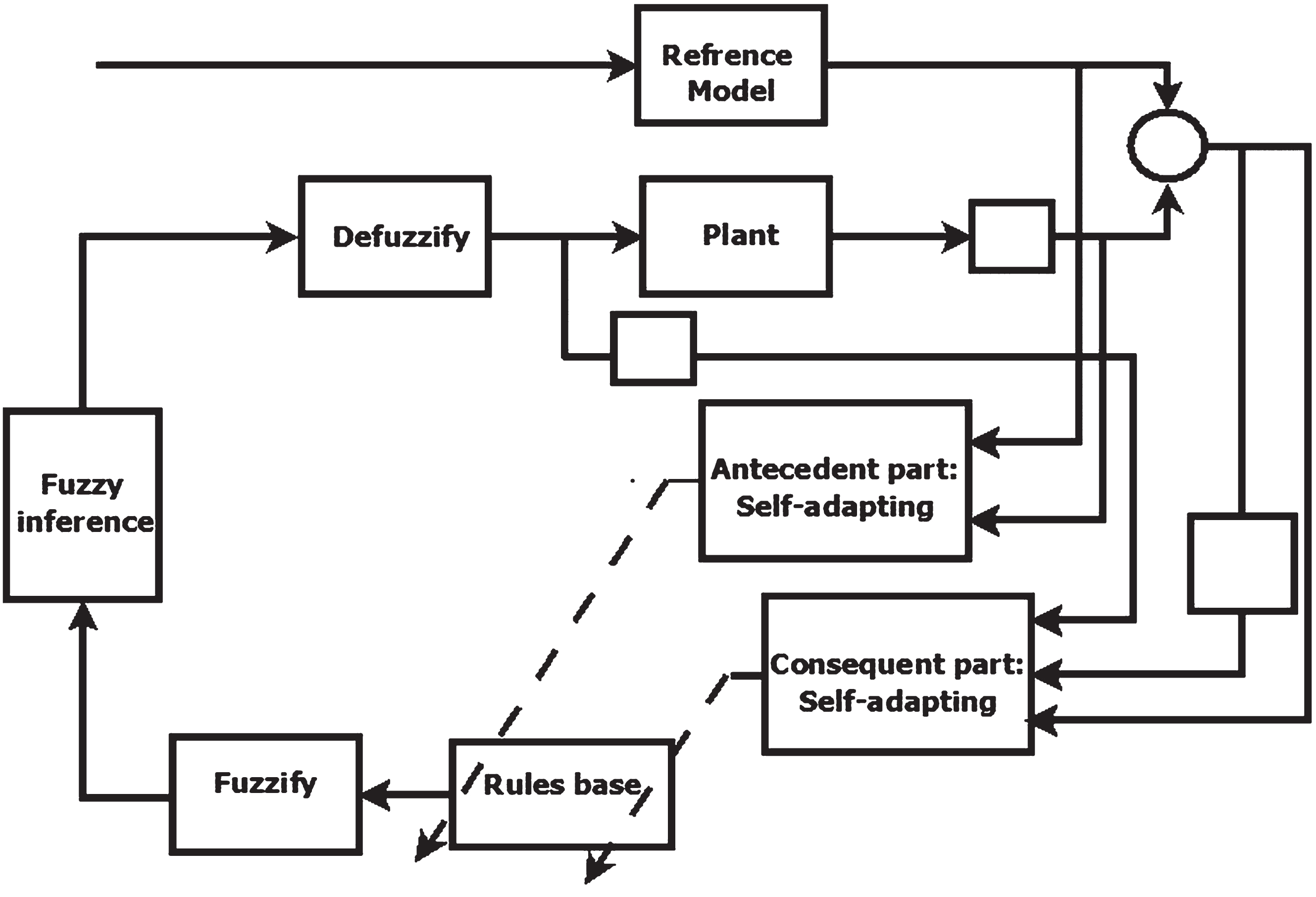
Self-adapting fuzzy controller block diagram.

$e (k) = y_{r} (k) - y (k)$ (1) $e_{b} (k) = y_{r} (k) - y (k - 1)$ (2)

The control signal at the kth time step is denoted by u (k) while e (k) and e_b (k) represent the error of the tracking and the error of optimization, respectively, at the kth sampling time step. e (k - 1) is the error at the k - 1th time step. The global structure of our approach is represented in Fig. 1.

2.1 Convolutional FLC

A typical FLC is depicted in Fig. 2, where the controller’s structure is realized through various combinations of input variables, membership functions, and rule bases. An optimized FLC configuration can be designed by selecting appropriate design parameters. Generally, the FLCs contain at least two inputs: error and rate of error. The output is a crisp value obtained by defining the connection between three steps: (1) transforming the linguistic variables using membership functions, (2) defining the aggregation using a rule base, and (3) defuzzifying the obtained output linguistic to obtain a numerical value [37].

Fig. 2

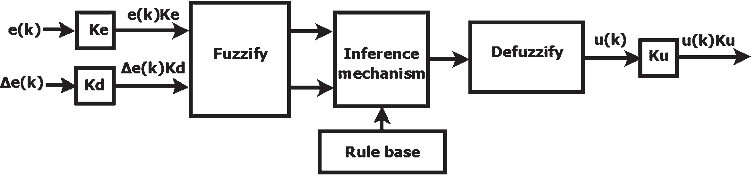
Convolutional FLC block diagram.

Observing Fig. 2, we can see that the incremental controller’s input scaling factors are K_e and K_d. While the output incremental FLC’s scaling factor is K_u. The outputs of the fuzzy controller depend on several factors, including the selection of membership functions (MFs), inference mechanism, input variables, defuzzification strategies (such as Mamdani and Takagi-Sugeno), and notably, the scaling factors K_e, K_d and K_u.

2.2 Self-adapting fuzzy control design

The self-adaptive fuzzy logic controller (SAFLC) has found extensive use in control applications as a learning algorithm for tuning scaling factors during the control evolution process. Generally, it begins with an assumed fuzzy rule base which is then adapted using a specific technique that does not require an explicit mathematical model of the system. As depicted in Fig. 1, the self-adapting algorithm proposed in this work involves changing the boundaries of membership functions based on performance measures and model estimation. Additionally, selecting the appropriate physical tuning factors is crucial to develop an effective decision table. However, creating a decision table for nonlinear control systems can be challenging, requiring skilled experts and knowledge bases. Therefore, integrating the self-adaptive fuzzy logic controller (SAFLC) with FLC methods is essential.

In the proposed SAFLC, the antecedent and consequent membership function (MF) limits are updated at each iteration to generate a new control increment. This adaptive mechanism solves the problem of an expansive database caused by the fixed range of the universe of discourse, thereby reducing the computational load and improving time efficiency.

Using the autoregressive moving average model, the system’s output behavior can be described by the following equation: $y (k) = \sum_{j = 1}^{N_{b} + 1} b_{j - 1} u (k - j) - \sum_{j = 1}^{N_{a}} a_{j} y (k - j)$ (3)

The variables y (k) and u (k) represent the output and input, respectively, at the k-step. The values of N_b and N_a are dependent on the dynamic characteristics of the system. In this work, we propose a technique for obtaining an optimal control sequence that enables the process to track a reference model.

In the previous convolutional fuzzy logic controller (FLC), the inputs can be either the error and the error rate or the required terms needed to compute the input u (k), such as y_r (k) , x (k) , x (k - 1) , x (k - 2) , . . . , u (k) , u(k - 1) , u (k - 2) , . . . , which are obtained from the inverse mapping of Equation (3) [33]: $\begin{matrix} u (k) = g (y_{r} (k), y (k), y (k - 1), . . ., \\ u (k - 1), u (k - 2), . . .) \end{matrix}$ (4)

Where y_r (k) is the output of the desired model.In all previous convolutional FLC strategies, the ranges of membership functions (MFs) are still assumed or calculated according to the term values of Equation (4). As a result, the MFs are preconstructed by experts or based on assumed range limits, which are unlikely to provide the required coverage of the space of fuzzification.

2.2.1 Definition of the self-adapting fuzzy controller’s input and output variables

(a) The antecedent part

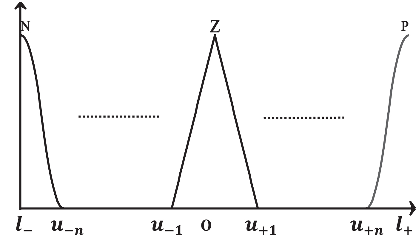
The proposed self-adapting controller has the advantage of accurately covering the input and output fuzzy set spaces. As depicted in Fig. 3, at each sampling time, the SAFLC uses either y (k - 1) or y_r (k) as input to design the membership functions within the Min_yr and Max_yr range, resulting in a one-dimensional space represented by a single membership function for the antecedent part.

Fig. 3

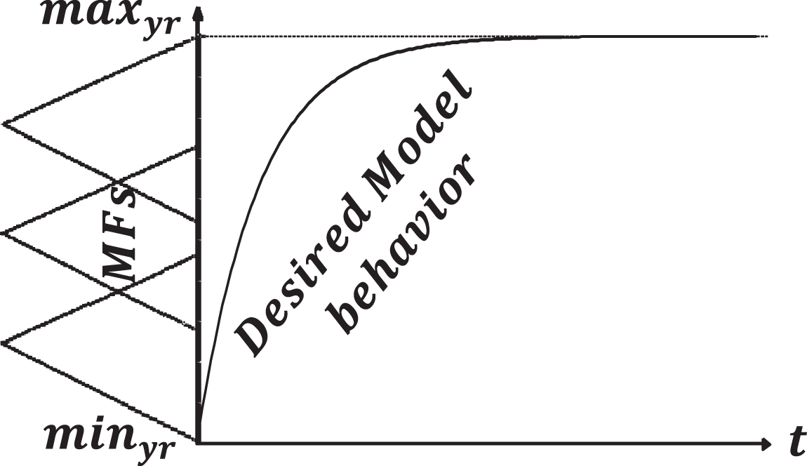
Example of input MFs limits: case of step response.

$μ_{i} (y (k - 1), y_{r} (k)) = ω_{i}$ (5)

Where ω_i is the rule applicability function.

(b) Consequent part

The membership functions describe one output variable in this part of the rules base. Although, at every kth step, the output MFs limits l (k) are arranged through a specific function that incorporates; e_b (k), Δe_b (k) and u (k - 1), expressed as: $l (k) = u (k - 1) + e_{b} (k) * Δ e_{b} (k) + sign (.) * λ$ (6)

It should be noted that the leading term of the function is the product e_b (k) * Δe_b (k), which accurately predicts the evolution of the control signal u (k) on a small scale.

The sign function denotes the left and right bounds of the membership functions, while the weighting factor λ corrects the membership functions range to prevent saturation of the value of u (k - 1). The value of λ is limited to the range of [0, 10^-α], where α represents the difference between u (k - 1) and e_b (k) * Δe_b (k) orders.

2.2.2 Fuzzification

Assuming the fuzzy system in Fig. 1 is a SISO system, where the input variables are dependent, and the output variables are independent, each rule can be expressed in a single input single output form. Equation (7) represents the rule base: $If y (y_{r}) is A^{i} then u is B^{i}$ (7)

At each sampling time, y or y_r serves as the input linguistic variable, with their values taken from fuzzy sets Aⁱ associated with the i^th rule, while, Bⁱ denotes the output fuzzy sets for the same rule. The number of the fuzzy rules represented by i = 1 … m.

Figure 4 describes the inputs (Min_yr, …, y_-1, y₀, y₊₁, … Max_yr) and outputs (l_min, …, u_-1, u₀, u₊₁, … l_max)) scaled factors of membership functions. Previous experimental studies of conventional FLC have demonstrated that various types and combinations of MFs result in different crisp output values for the same objective. However, this problem can be resolved by the proposed self-adapting technique, which eliminates the impact of MF types on the output control signal.

Fig. 4

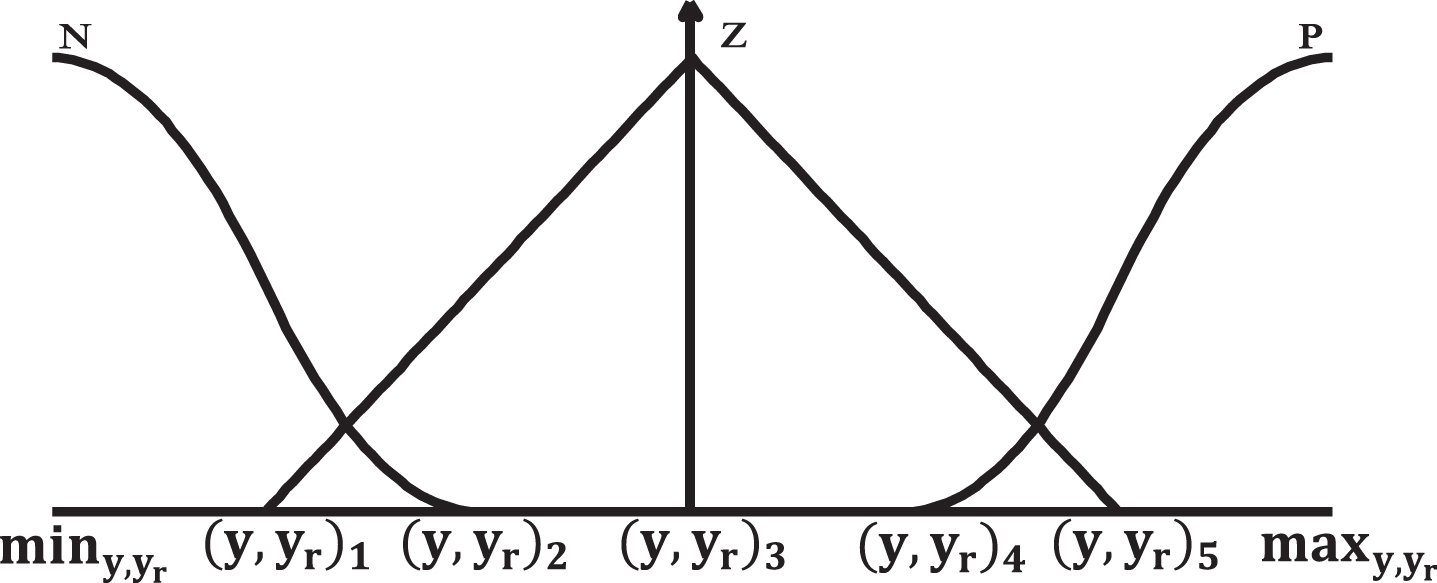
MFs of input variables.

The linguistic variables and their fuzzy sets (Aⁱ, Bⁱ) are typically determined based on prior experience in a fuzzy controller. However, in our proposed approach, the input fuzzy sets Aⁱ will be updated at each sampling step using the values of y (k - 1) and y_r (k) as it is depicted in Fig. 3. For output fuzzy sets Bⁱ, the output they will be designed based on the values of u (k - 1), e_b (k) and Δe_b (k) using the updated limits of Equation (6). The fuzzification module operation converts the scaled input and output variables into fuzzy linguistic control variables such as NF’, ‘NM’, ‘NC’, ‘Z’, ‘PC’, ‘PM’, ‘PF’, ‘C’, ‘M’ and ‘F’.

The membership functions used can be one of the different types, such as trapezoidal, triangular, Gaussian, and so on. The input variable is divided into at least three fuzzy sets: negative, zero/medium, and positive, as depicted in Fig. 4, to ensure complete coverage of the input and output variable space with MFs for obtaining the appropriate control signal. The Gaussian and triangular types are used for describe the input MFs of y (k - 1) and y_r (k), while the triangle type represents the output. $μ_{Z} (y (k - 1)) = {\begin{matrix} \frac{y_{r 5} - y}{y_{r 5} - Y_{0}} & if & y_{r 0} ⩽ y ⩾ y_{r 5} \\ \frac{y - y_{r 1}}{Y_{0} - y_{r 1}} & if & y_{r 1} ⩽ y ⩾ y_{r 0} \\ 1 & if & y = y_{r 0} \end{matrix}$ (8) $μ_{C} (y (k - 1)) = {\begin{matrix} 0 & if & y ⩽ y_{r 4} \\ 2 {(\frac{y - y_{r 4}}{MaxYref - y_{r 4}})}^{2} & if & y_{r 4} ⩽ y ⩾ ma x_{y_{r}} \\ 1 & if & y ⩾ ma x_{y_{r}} \end{matrix}$ (9) $μ_{F} (y (k - 1)) = {\begin{matrix} 1 & if & y ⩾ mi n_{y_{r}} \\ 1 - 2 {(\frac{y - mi n_{y_{r}}}{mi n_{y_{r}} + y_{r 2}})}^{2} & if & mi n_{y_{r}} ⩽ y ⩾ y_{r 2} \\ 0 & if & y ⩾ y_{r 2} \end{matrix}$ (10)

The remaining membership functions can be determined using the same approach. It’s worth noting that the number of fuzzy sets is not fixed, but in this study, we considered three and nine membership functions to describe the input and output variables, respectively. The scaled factors ((y, y_r) ₁, … (y, y_r) ₅ and u_-n, … u_+n) are calculated at each sample time based on the values of y (k - 1) and y_r (k) within the ranges of [min x_{y
_r}, $\max_{y_{r}}$ ] for the input, and the value of e_b (k) , Δe_b (k) and u (k - 1) within the ranges of [l_-, l₊] for the output. As shown in Fig. 5, the output membership functions are designed with a symmetric slope, where l_- and l₊ represent the left and right lines, respectively. One advantage of the adopted fuzzification operation is that it requires minimum data to construct the membership functions.

Fig. 5

MFs of output variables.

2.2.3 Rules base

Table 1 shows the rule base for the controller. The multiple input and output membership functions are fuzzified using triangle and Gaussian functions. The fuzzy membership linguistic variables, such as “NF” for “Negative Far,” “NM” for “Negative Medium,” “NC” for “Negative Close,” “Z” for “Zero,” “PC” for “Positive Close,” “PM” for “Positive Medium,” “PF” for “Positive Far,” “C” for “Close,” “M” for “Medium,” and “F” for “Far,” are defined for the purpose of the controller’s design.

Table 1
SAFLC rule base

Rules # IF

y (k)/y_ref (k) THEN u (k)

Response is below the reference C – PC

M – PM

F – PF

Response is above the reference – C NC

– M NM

– F NF

Response matched on the reference C C Z

M M Z

F F Z

Rules #	IF
Response is below the reference	C	–	PC
	M	–	PM
	F	–	PF
Response is above the reference	–	C	NC
	–	M	NM
	–	F	NF
Response matched on the reference	C	C	Z
	M	M	Z
	F	F	Z

As shown in Equations (6), the input-output membership function base location and centroid are organized in every case considered. The scaled factors ( and l₊) are tuned to ensure that the fuzzy controller produces the optimal output for the controlled system. $u_{opt} \in [l_{-}, l_{+}]$ (11)

From the rule base and Fig. 6, it can be observed that the input variable is either y (k - 1) or y_r (k). For instance, if the input variable is y (k - 1), y_r (k) is used as the boundary of the membership function input space, and vice versa. In the third case, the rule outcomes are identical. These two rules can be combined into one using the OR operator. Figure 6 illustrates all possible combinations of the fuzzy controller’s input variables (y and y_r), creating four main areas with dashed lines on the scaled input planes. Consider the first and second regions: the input MFs limits are $[\min_{y_{r}}$ , y (k - 1)] and [y (k - 1), $\max_{y_{r}}]$ , respectively, since y (k - 1) is outside the reference model bounds, whereas y_r (k) is used to determine the rule degree value to find the control value that decreases/increases y (k - 1) backward/toward y_r (k). For the third and fourth regions, the input MFs limits are $[\min_{y_{r}}$ , y_r (k)] and [y_r (k), max_{y
_r}], respectively, because of y (k - 1) is within the reference model bounds and is lower than y_r (k), in this case; y (k - 1) is used to determine the rule degree value that enables increasing/decreasing y (k - 1) toward y_r (k).

Fig. 6

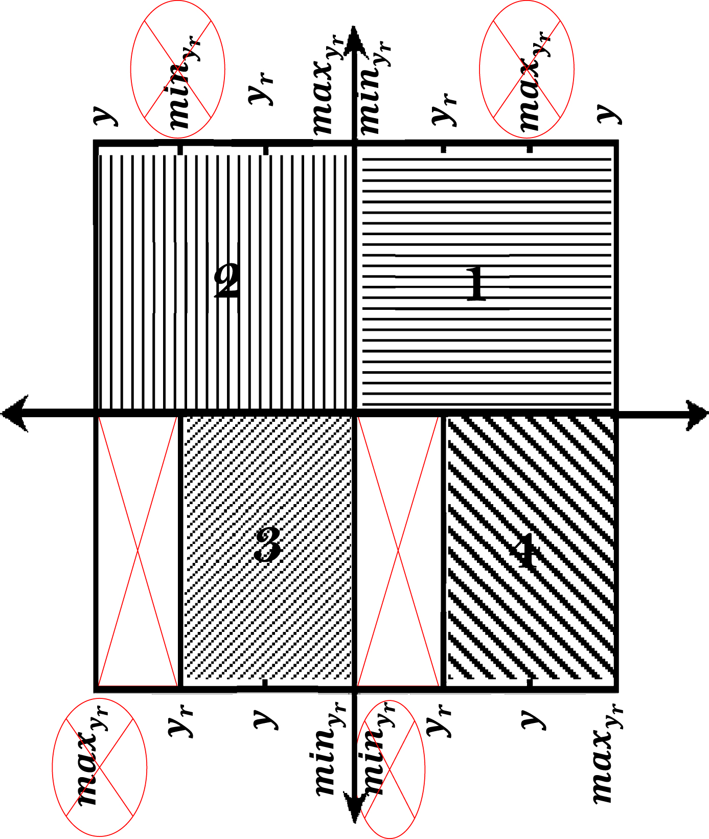
Regions of scaled input planes of fuzzy controller.

2.2.4 Inference mechanism

The limits of the output membership functions are adjusted based on the results obtained from the antecedent part at each sampling time, as shown in Equation (6), which allows having potential control values and helps to ensure that the controller can effectively regulate the system. By dynamically modifying the membership function limits, the fuzzy controller is able to adapt to changes in the system dynamics and respond in a timely and effective manner.

Figure 7 provides an example of the output fuzzy sets and their corresponding degrees of membership (ω). It can be seen that the limits of the output membership functions are updated at each time step, based on the new position of the input fuzzy sets, as shown in (Equation (6)). Notably, the compositional rule of inference does not involve the use of the min and AND operators in this proposed technique. Instead, the membership degrees ω_i and ω_i+1 are immediately determined by computing the membership degree of the input fuzzy set concerning each rule’s antecedent linguistic values (y (k - 1) or y_r (k)). As illustrated in Fig. 7, this process considers the degree of intersection between the input fuzzy variable and the antecedent linguistic values. At each step, the membership degrees ω_i and ω_i+1 are determined based on the contribution of one input variable. The consequent linguistic value B_i is computed by taking the α-cut of the B_i.

Fig. 7

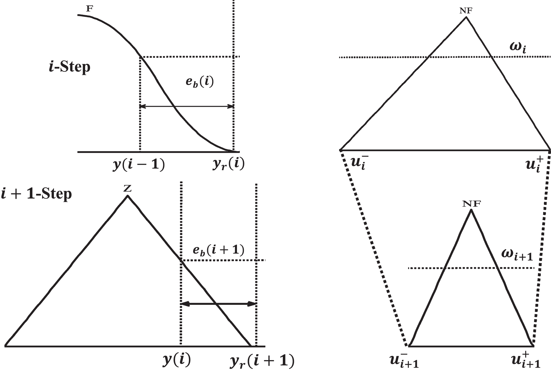
Inference MFs of fuzzy sets on scaled input/output variables.

2.2.5 Defuzzification

Defuzzification is the process of converting a fuzzy output into a crisp value. Several defuzzification strategies are available, with the center of gravity (COG) method and the mean of the maximum (MOM) method being the most commonly used. From a practical perspective, not all control values within the proposed output MFs space have a potential. Many studies have demonstrated that the COG method is more accurate than other defuzzification methods [38]. In the CoG method, the overlapping region between two adjusted MFs is only counted once, making it the most commonly used method in developing fuzzy controllers. In this work, the authors proposed a new technique with dynamic space of input/output MFs, in which the COG defuzzification method is used to determine the crisp value of the control increment.

Because each membership function has equal-sized partitions, the computed control values within the membership function boundaries resulting from the inference have the same potential to be used as a control. However, it is essential to note that not every control value within the membership function boundaries may be practical or effective in achieving the desired control objective.

The final crisp control value, u (k) s obtained using the COG defuzzification method applied to the modified output MFs boundaries, as illustrated in Fig. 7.

Figure 8, Od represents the order of the fuzzy set points within the MF boundaries, while n denotes the number of output MFs used. The CoG defuzzification method allows us to obtain the crisp values of the control efforts from the inferred MFs on the output variables. Specifically, the COG method calculates the center of gravity of the output MFs and returns this value as the crisp control output as follows:

Fig. 8

Reference and inferred MFs of fuzzy sets on scaled output variables.

$u^{*} (k) = \frac{\sum_{l_{-}}^{l_{+}} μ_{Ri} u (k)}{\sum_{l_{-}}^{l_{+}} μ_{Ri}}$ (12)

2.2.6 Self-adapting algorithm

The input space partitioning by the proposed self-adaptive fuzzy controller is calculated in a single step and updated at each sampling time. Specifically, at each sampling time, the controller generates new divisions of the input membership functions (MFs) within the range of [ min _{y

_r}, max _{y

_r}] and stores them in the rule base. This mechanism allows the controller to adapt to changes in the input distribution over time. However, for the consequence part, the membership functions (MFs) are updated based on the error and the error variation. This leads to a single output MF associated with multiple corresponding input MF partitions. Consequently, the number of MF bounds stored in the rule base is reduced, which helps avoid memory exhaustion problems. The fuzzy rule space is partitioned according to the desired model discretization number, resulting in a limited space of different sizes for each rule stored at each sampling time. The input variables consist of a single variable, which can be either y (k - 1), or y_r (k) at each sample time. Therefore, if y_r (k) is considered the input variable, then the corresponding y (k - 1) is automatically used to determine the rule degree, and vice versa.

Several distinguishing features characterize our control design approach.

One key difference is using a single input variable (either y or y_r) instead of the two input variables (error and rate of error) commonly used in classical convolutional FLC. This simplification of the input space reduces the complexity of the control system and allows for more efficient and effective control of the process. By relying on a single input variable, our approach can achieve comparable or better performance with less computational effort and fewer tuning parameters, making it a more practical and reliable solution for real-world applications.

The rule base is updated dynamically as the control system evolves by changing the membership function (MF) bounds. This allows the system to adapt to the changing dynamics and improve its performance.

The fuzzy sets of the rule space can be the same for different set-points, simplifying the control design process and reducing computational requirements.

The linguistic value ranges for inputs and outputs are determined at each sample time rather than being assumed, enabling more precise control and greater flexibility.

For certain set-points, inputs or outputs may be fuzzified using the same ranges, further simplifying the control system and improving efficiency.

Our approach differs from previous fuzzy controller methods in that there is no need for an operator (such as END) in the inference mechanism, making it more straightforward and effective.

The rule ensures the minimal value of the cost function is selected for the same output, as shown in Fig. 9.

Our proposed updating fuzzy control method can learn the object plant and self-adapt the rule base, improving the system’s adaptability and robustness.

The number of input and output MFs limits is related to the number of set-points, and it will be increased as additional data is encountered. However, the maximum number of MF partitions in the rule space never exceeds the number of output set-points, ensuring efficient and effective control.

Fig. 9

Process for updating the rules base.

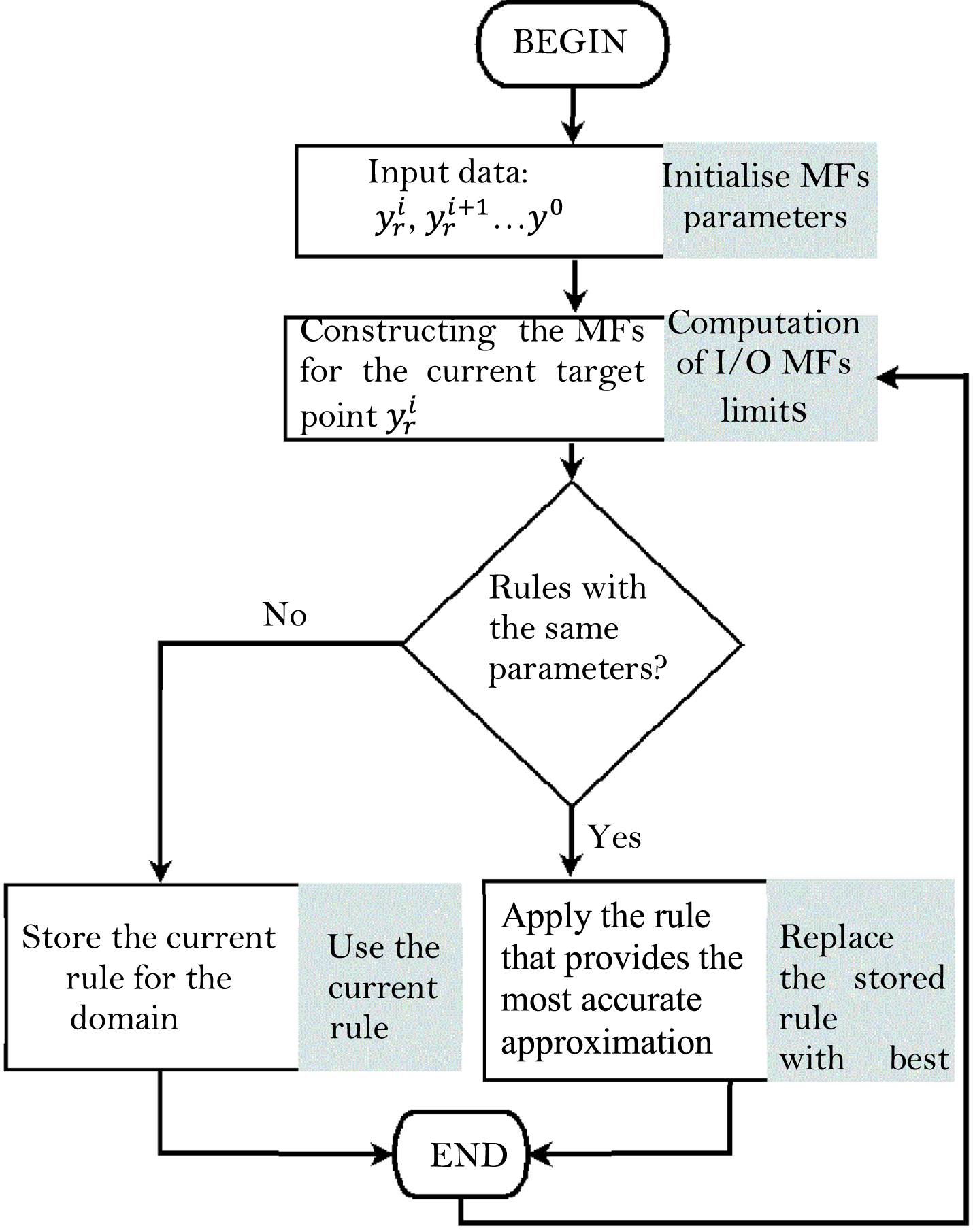
The following global algorithm describes the self-adapting fuzzy controller approach mentioned previously.

Algorithm 1: algorithm for self-adapting fuzzy controller
Data:available data set
$T = y_{ref}^{1}, y_{ref}^{2}, \dots, y_{ref}^{N}, r^{1}, r^{2}, \dots, r^{N}, y^{1}$ , λ
Begin:initialisation phase
– Determine the maximum and minimum crisp values of
y_ref and u, detonated as y_refmin, y_refmax, $l_{-}^{i}$ , $l_{+}^{i}$
– Generate the linguistic values of each input and output
based on these limits, using the determined values as
the modal values, i.e.,
L { y } = { A_i } , L { y_ref } = { B_i } , L { u } = { C_i } ,
– Construct the initial rule base using the inference
mechanism described in sect. 4 and illustrated in Fig. 6.
For each point $(y_{ref}^{i}, y^{i - 1}) \in T$ do
Repeat:apply the fuzzy model to the input $(y_{ref}^{i}, y^{i - 1})$ and get the corresponding outputuⁱ
$u^{i} = fuzzyModel (y_{ref}^{i}, y^{i - 1}, l_{-}^{i}, l_{+}^{i}, y_{refmin}, y_{refmax})$
yⁱ = plant (y^i-1, uⁱ)
// compute the errore_bⁱas the difference between the reference model output and the plant response.
${e_{b}}^{i} = y_{ref}^{i} - y^{i - 1}$
Δe_bⁱ = e_bⁱ - e_b^i-1
For all previous $y_{old}^{i}$
If If there is a stored rule with the same output yⁱ, and the value of yⁱ for the old rule is smaller than that for the new rule, then the old rule takes precedence over the new one.
Then $l_{-}^{i} = l_{- old}^{i}$ , $l_{+}^{i} = l_{+ old}^{i}$
Else // determine the new output fuzzy set limits using Eq. (6)
$l_{-}^{i} = - \| u^{i - 1} + {e_{b}}^{i} * Δ {e_{b}}^{i} - λ \|$
$l_{+}^{i} = \| u^{i - 1} + {e_{b}}^{i} * Δ {e_{b}}^{i} + λ \|$
Endif
Endfor
Ifeⁱ > e^SC// desired accuracy not achieved, apply the strategy described in Sect. 4 to the same point $(y_{ref}^{i}, y^{i - 1})$ using the new output fuzzification limits
Endif
Untileⁱ ⩽ e^SC
// repeat the control phase until the maximum errore^SCis reachd
Endfor
End

The following steps summarize the proposed self-adapting fuzzy control method:

Step 1: prepare input variables and parameters.

In this step, the input data is determined, which includes the input and output of the reference model.

Step 2: built initial rules base

The initial limits of the input and output fuzzy sets are determined from previous data. Based on these limits, one linguistic value is assigned to the input and output space, providing the initial rules base.

Step 3: evaluate the fuzzy control model

This step uses the current fuzzy control model to compute the control crisp value uⁱ and the plant response yⁱ. If the error eⁱ between the current response yⁱ plant and $y_{r}^{i}$ is less than a predefined threshold, move to step 4 and then step 3 with the new reference output $y_{r}^{i + 1}$ . If the error eⁱ exceeds the threshold, repeat step 3 with new input-output limits from Sec. 2.2.1.

Step 4: modify the rule base

In this step, the rules with the same parameters are reorganized. If a previous rule exists with the same output and the output is smaller than the current rule, the previous rule’s parameters are used, and vice versa. This reorganization mechanism allows the fuzzy controller model to learn about the worst and best performance of MFs parameters during the control process. Figure 9 shows the rule base updating procedure.

Since there are no errors or rate errors in the rule base, the output MFs for the first step are limited to the minimum and maximum values of the model reference set-point.

The input and output linguistic variables used to control the plant remain unchanged at each sampling time. However, the crisp value in the antecedent part can be yⁱ and $y_{r}^{i}$ depending on which of the four cases depicted in Fig. 6 the MFs boundaries belong to. This algorithm creates fuzzy set shapes at each sampling time to produce zero tracking error for target points. Even if new rule parameters don’t always decrease the maximum tracking error, they can still be updated or replaced to ensure zero error.

3 Simulation results and discussion

The effectiveness of the proposed approach has been demonstrated through simulation studies of two real-world systems that are nonlinear and subject to time delays.

3.1 SAFLC control of a nonlinear internal system

Consider the following process to be simulated by the discrete-time equations: ${\begin{matrix} x_{p} (k) = H (x_{p} (k - 1), x_{p} (k - 2), u (k - 1)) \\ y_{p} (k) = 4 tanh (\frac{x_{p} (k)}{4}) \end{matrix}$ (13)

Where y_p (k) represents the output of the process, u (k) denotes the control signal, and the function H is given by: $H (h_{1}, h_{2},, h_{3}) = h_{1} \frac{24 + h_{1}}{30} - 0.8 \frac{24 + {h_{3}}^{2}}{{h_{3}}^{2}} h_{2} + 0.5 h_{3}$ (14)

This system has been used as a reference in several papers to evaluate different control strategies due to its multiple behaviors. The system’s behavior changes according to the operating points (u₀, y₀): around (0,0), it behaves like a damped first-order filter. However, the behavior becomes more complex at operating points that include large amplitudes of u₀. Moreover, if the operating points lie within the range of 0.1 〈 u₀ 〉 0.5, the behavior becomes more oscillatory [39].

The proposed SAFLC-based fuzzy control was tested using a sequence of pulses with random amplitudes in the range of [-0.5, 0.5] and random durations between 40 and 90 sampling steps as the set-point.

The proposed SAFLC-based fuzzy control was tested using a sequence of pulses with random amplitudes in the range of [-0.5, 0.5] and random durations between 40 and 90 sampling steps as the set-point. The sequence had a total length of N = 300. The behavior of the control system based on the proposed SAFLC approach is shown in the figures below. The control signal is obtained by minimizing the following objective function: $J_{cost} = ISE = \sum_{i = 1}^{N} {(y_{r}^{i} - y^{i})}^{2}$ (15)

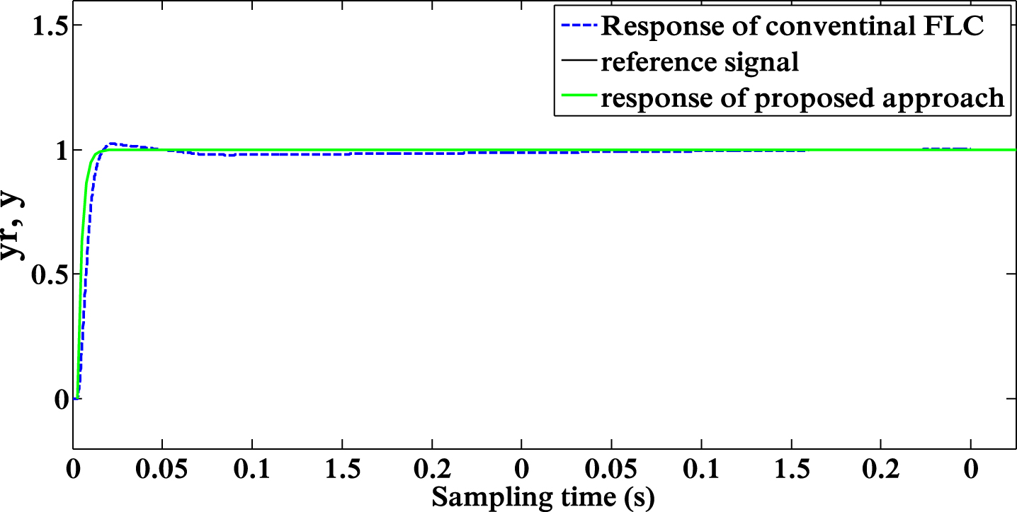
The variables $y_{r}^{i}$ and yⁱ represent the output of the reference signal and controlled system, respectively, with N referring to the sequence length.

The proposed SAFLC controller generates the control signal for tracking the desired model response. Table 1 shows the controller’s rule base, while the input and output membership functions (MFs) are fuzzified using Equations (6), and (10). The controller uses triangle membership functions, with three for the antecedent part and seven for the consequent part, as shown in Fig. 10. Algorithm 1 is used to determine the control signal applied to the process. Figure 13 shows the reference model (y_r) and the outputs of the controlled process (y) using SAFLC and conventional FLC. The control signal applied to the process (u) and the control error are shown in Figs. 11 12, respectively.

Fig. 10

(a): antecedent and (b): Consequent DFs for system controllers.

Fig. 13

Desired response signal (y_r) and controlled system response (y) using proposed approach SAFLC for optimized boundaries.

Fig. 11

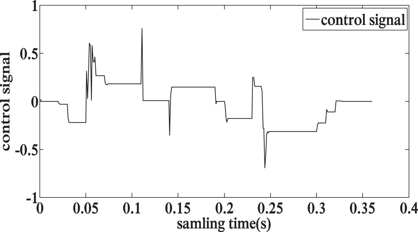
Control signal.

Fig. 12

The instantaneous control error.

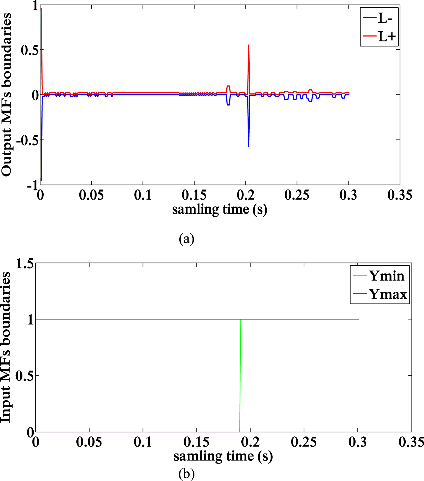
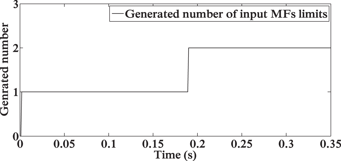
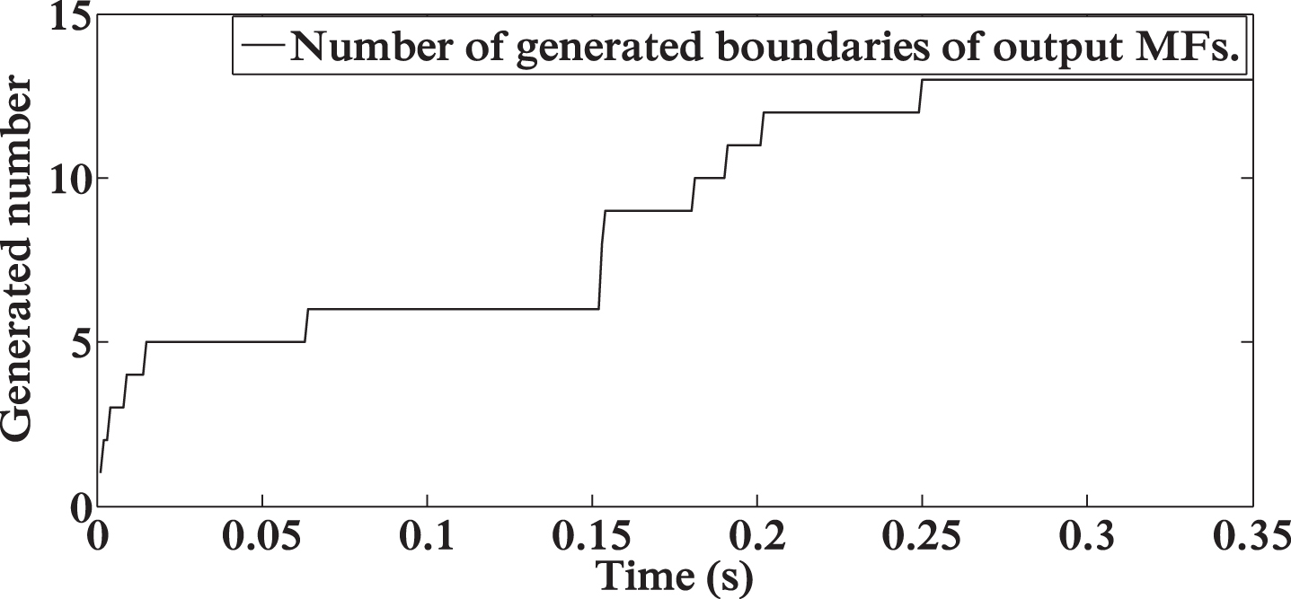
The variations of the MFs limits are presented in Fig. 14, and it is noted that the behavior of the controlled process is the same as the model reference at each sampling time. The number and value of the input/output MF limits at each sampling time are shown in Figs. 15 16, respectively. It’s worth noting that the algorithm starts with membership functions that are uniformly distributed within a random range, and the number of limits increases according to the instant evolution of the reference signal.

Fig. 14

(a) Output membership functions boundaries (b) input membership functions boundaries.

Fig. 15

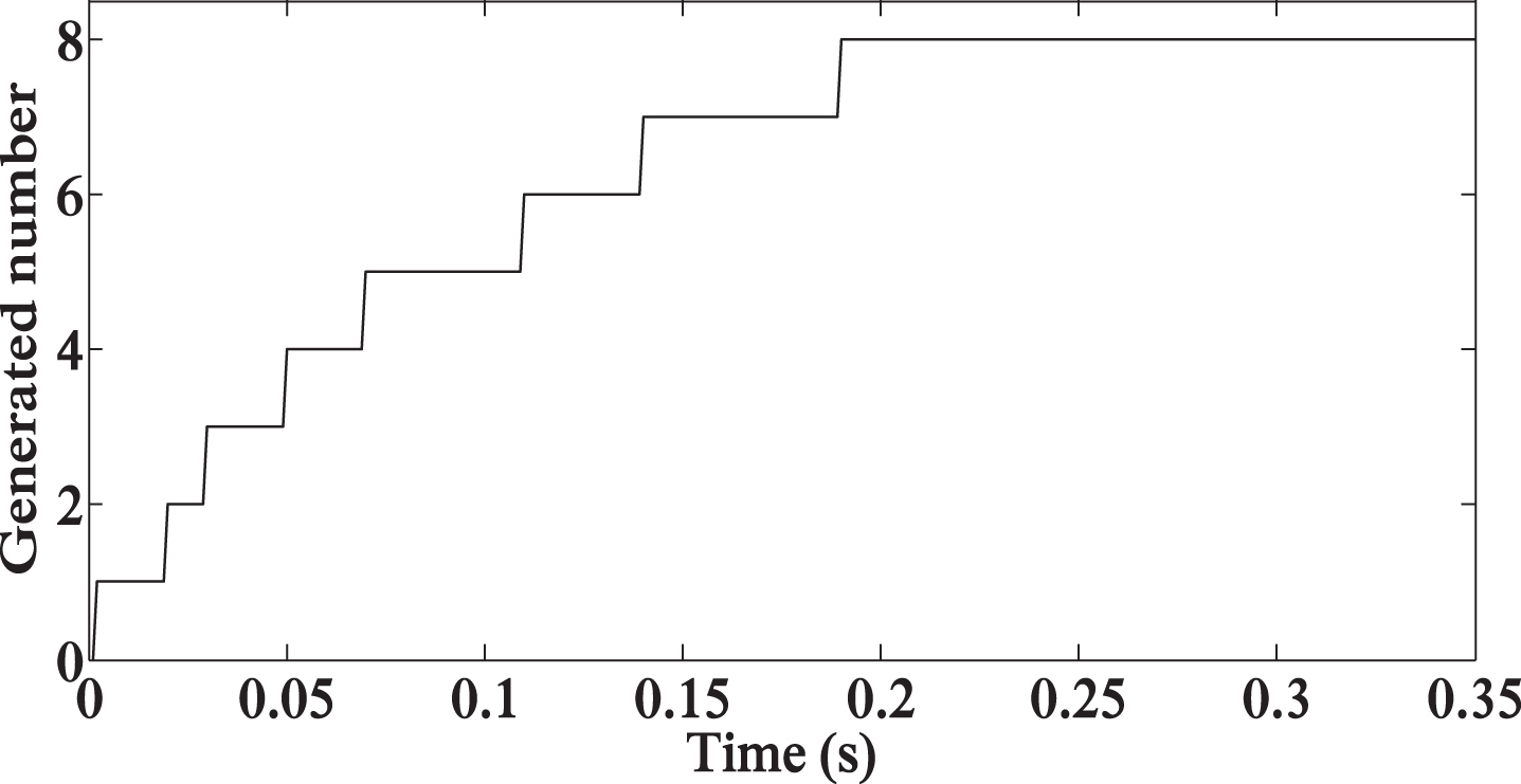
Number of generated boundaries of input MFs.

Fig. 16

Number of generated boundaries of output MFs.

3.2 SAFLC Control of a Sun tracker system

The sun-tracker system utilizes two PV cells as a current source to generate an output when sunlight is projected onto them. The system’s output is the electric current, which is proportional to the luminous intensity diffused on the PV cells. The input is a voltage signal produced by both cells, which is then fed to a DC motor drive system. The motor drive system rotates the PV cell until it is vertically aligned with the sunlight to achieve a zero error voltage, and then the DC motor is turned off [40]. The dynamic model of the sun-tracker system, which describes the relationship between the output gear angular position and the position of the motor, can be represented by the following state space equation: $\begin{matrix} [\begin{matrix} {\dot{x}}_{1} \\ {\dot{x}}_{2} \end{matrix}] = [\begin{matrix} 0 & 1 \\ 0 & - \frac{1}{τ_{c}} \end{matrix}] \\ y = [1 0] {[x_{1} x_{2}]}^{T} \end{matrix} [\begin{matrix} x_{1} \\ x_{2} \end{matrix}] + [\begin{matrix} 0 \\ \frac{k}{τ_{c}} \end{matrix}] u .$ (16)

As given by Equation (17), the open loop transfer function is derived from the system’s state space representation by disregarding the static nonlinearity and characterizing the model as an output of desired position. $G_{ST} (s) = \frac{M_{s} K}{s (τ + s)}$ (17)

The servo gain amplifier, denoted as K and set to a value of 1, and the error discriminator constant, denoted as M_s and fixed at 1.5625 x 10^-2, are included in the expression for the open-loop transfer function, as given in Equation (17).

The sun tracking system is controlled by a fuzzy controller based on Algorithm 1. The reference model consists of a step response from a stable first-order system. Figure 17 displays the control signal variation (u), and Fig. 19 shows the control error between the PV and sunlight axis. The controller generates successive impulses to rotate the system’s photovoltaic (PV) axis toward the ideal solar axis position.

Fig. 17

Control signal.

Fig. 19

The instantaneous control error.

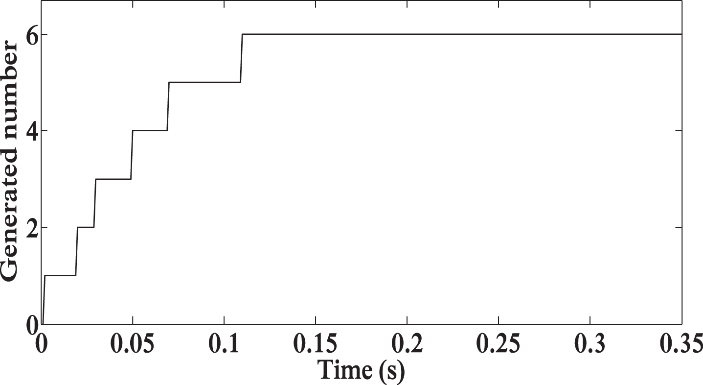
Figure 18 shows the reference model response (y_r) and the outputs of the controlled process (y) using SAFLC and conventional FLC. The variation of the membership function boundaries and the number of limitations generated by the fuzzy controller are shown in Figs. 20 –22.

Fig. 18

Desired response signal (y_r) and controlled system response (y) using the proposed approach SAFLC for optimized boundaries.

Fig. 20

(a) Output membership functions boundaries (b) input membership functions boundaries.

Fig. 21

Number of generated boundaries of input MFs.

Fig. 22

Number of generated boundaries of output MFs.

3.3 Robustness test

A robustness test is a crucial step in evaluating the effectiveness of the proposed control method. This test involves subjecting the control system to a range of disturbances and uncertainties in order to assess how well it can maintain stable and accurate control under less-than-ideal conditions.

In this work, a robustness test is applied to determine whether the control method can handle unexpected system or external environment changes and still function within acceptable performance limits. The robustness test results are essential for determining the practicality of the new control method in real-world applications. If the system proves robust under a wide range of conditions, it may be considered a viable candidate for implementation. On the other hand, if the system shows poor performance in the face of disturbances, further refining or improving the control algorithm may be necessary before using it in practical applications.

To assess the robustness of our proposed fuzzy controller, we subjected it to a modified process dynamics scenario to test if it could adapt to new system dynamics and track a desired reference model sequence. A disturbance was introduced to the process parameters at two different times: 0.05 seconds and 0.13 seconds. The first disturbance increased the process parameters by 40%, while the second decreased them by the same amount. These instants pose a risk of causing a runaway situation. Although all system parameters were modified with the same percentage at each instant, their effect on the process behavior was different.

3.4 Results discussion

The simulation results indicate that our approach and FLC convolutional are able to efficiently track the reference signals for the internal nonlinear system. However, the control tracking performance of the two methods can be compared based on their tracking error and overshoot. Our proposed approach, SAFLC, exhibits a significantly lower minimum tracking error of 1.4 x 10^-6 compared to FLC convolutional, which has a minimum tracking error of 8.1 x 10^-2. Furthermore, SAFLC has a lower maximum tracking error of 1.9 x10^-5 compared to FLC.

In terms of overshoot, SAFLC has a value of 0%, indicating that it accurately tracks the reference signal without any oscillations. In comparison, FLC has an overshoot of 8.0%, suggesting may exhibit some instability in its tracking behavior. The superiority of SAFLC in control tracking performance is further supported by the comparison of results shown in Fig. 13 and Table 2.

Table 2
Simulation results of the controlled Internal nonlinear system using SAFLC and Conventional FLC methods

system\Parameters Approaches Error minimization Max Input Output

value Overshoot (%) Boundary Boundary

Internal nonlinear system SAFLC (weight factor λ = 0.1) 1.4x10^-6 0.0% [-0.5→0.1, 0→0.65] [-0.5→0, 0→1.9]

Conventional FLC 8.1x10^-2 8.0% e[-10, 10] [-10,10]

Δe[-1,1]

system\Parameters	Approaches	Error minimization	Max	Input	Output
Internal nonlinear system	SAFLC (weight factor λ = 0.1)	1.4x10^-6	0.0%	[-0.5→0.1, 0→0.65]	[-0.5→0, 0→1.9]
	Conventional FLC	8.1x10^-2	8.0%	e[-10, 10]	[-10,10]
				Δe[-1,1]

Therefore, based on the results, our proposed approach, SAFLC, outperforms FLC convolutional in control tracking due to its significantly lower tracking error and absence of overshoot, indicating that it can accurately track the reference signal with improved stability.

For the sun tracker system, the control tracking of our SAFLC approach and FLC convolutional can be compared based on their tracking error, overshoot, and settling time. SAFLC outperforms FLC in terms of tracking error, with a lower range of tracking error, ranging from a minimum of 9.0 x 10^-5 to a maximum of 1.8 x 10^-4, compared to FLC’s higher tracking error of 2.1 x 10^-2. Additionally, SAFLC has a settling time of 0.1538 seconds, which is higher than the settling time of FLC, which is 0.0098 seconds. Regarding overshoot, SAFLC accurately tracks the reference signal without any oscillations, with an overshoot value of 0%, while FLC has an overshoot of 2.4% (in Fig. 18 and Table 3).

Table 3

Simulation results of the controlled Sun tracker system using SAFLC and Conventional FLC methods

system\Parameters	Approaches	Error minimization value	Max Overshoot (%)	Settling time (sec)	Input Boundary	Output Boundary
Sun tracker system	SAFLC (weight factor λ = 0.01)	9.0x10^-5	0.0%	0.0098	[0→0,1→1]	[0→-0.95, 0→0.96]
	Conventional FLC	2.1x10^-2	2.4%	0.1538	e[-10, 10] Δe[-1,1]	[-3.33,3.33]

Based on these results, SAFLC appears to have more consistent and accurate control tracking performance than FLC, despite its longer settling time. The absence of overshoot and lower tracking error range are strong indicators of SAFLC’s superiority over FLC. However, it’s worth noting that FLC has a shorter settling time, which may be a crucial factor in specific applications. Therefore, the choice of method would depend on the system’s.specific requirements, such as the desired accuracy, speed, and stability of the control tracking.

In summary, the comparison of results suggests that our approach is preferable for systems that require high accuracy and stability, at the same time, FLC is better suited for applications where fast settling time is crucial, but with a potential tradeoff in tracking error and overshoot.

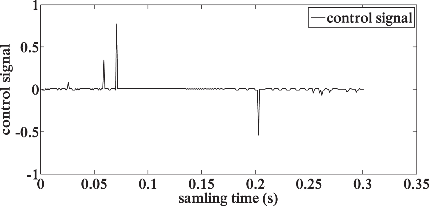
The robustness test of our control method is shown in Fig. 23 by changing the internal nonlinear system’s parameters by±40%. The output-controlled system successfully tracked the reference model after a small oscillation with a static average error of only 0.009. This error was maintained at 10^-5 after that, indicating that the control method was stable and efficient. Although there were surpassing peaks due to disturbances in the parameters, they were considered acceptable. It is worth noting that the control method recovered quickly and followed the desired set-point after a temporary runaway situation that lasted for only 0.02 seconds (equivalent to six iterations). This capability demonstrates that the proposed fuzzy controller calculation mechanism can adapt to new process dynamics and sudden changes in system parameters. Thus, it is well-suited for any nonlinear system without requiring optimization techniques. The results of the testing suggest that the control method is robust and has the potential to perform well in real-world applications. However, the magnitude and timing of disturbances may affect their performance. Therefore, further testing and analysis are necessary to fully understand its robustness in different scenarios. Overall, the proposed control method shows very satisfying results, and it has the potential to be a valuable tool for engineers and researchers working in the field of control systems.

Fig. 23

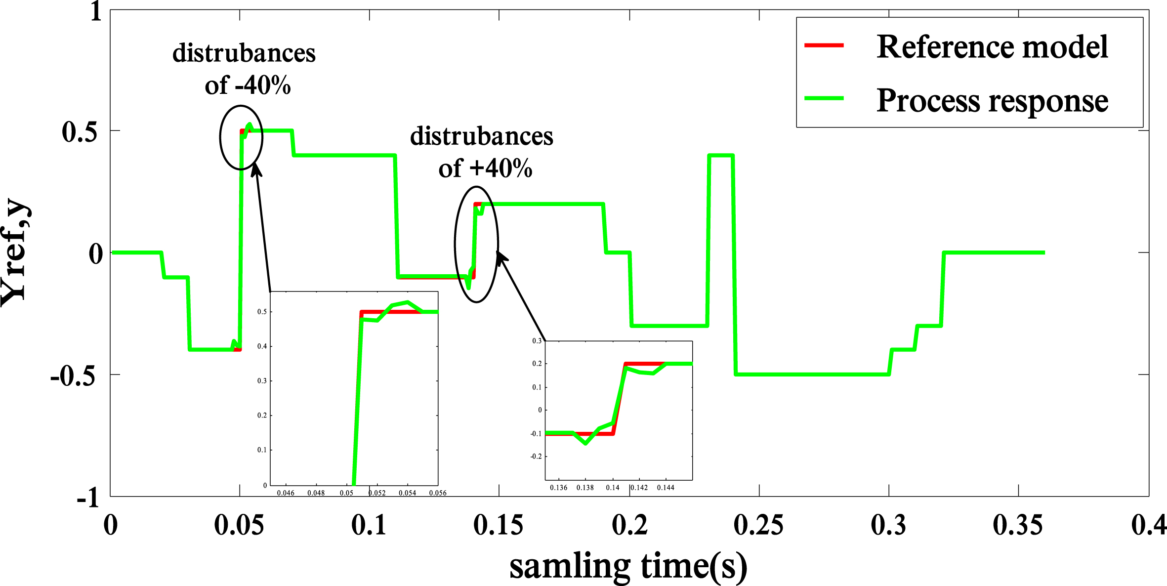
Response of controlled Nonlinear Internal System with disturbance.

According to the obtained results summarised in Tables 2 3, Another significant advantage of the SAFLC method over the conventional FLC method is the use of dynamic MF boundaries for both the input and output variables. For the internal system, the SAFLC method uses a single input variable with a variable limit of [-0.5 to -0.1, 0 to 0.65], and the input boundary variation number is 8; This means that the input variable boundary changes based on the input data, and eight possible combinations of the input boundaries that can be used during the control process. Similarly, the SAFLC method uses one output with a variable limit of [-0.5 to 0, 0 to 1.9], and the output boundary variation number is 6; this means that the output boundary changes dynamically based on the output data, and six possible combinations of the output boundaries that can be used during the control process. In contrast, the conventional FLC method uses two input variables with fixed boundaries of [-10; 10] and error variation with fixed boundary [-1, 1], with no variation in the input or output variable boundaries.

The dynamic MF boundaries of the SAFLC method allow for more adaptive and flexible control, leading to better tracking performance.

Overall, the SAFLC method with dynamic MF boundaries outperforms the conventional FLC method with fixed MF boundaries in terms of tracking performance, stability, and adaptivity. As shown in (Figs. 15 , 21 and 22), the impact of the system dynamics and reference model on the number of boundaries can be seen in the two different systems being considered. In System 1, a Nonlinear Internal System with a random square signal as the reference model, there are eight boundaries in input and six in output. The system dynamics, in this case, are likely more complex and difficult to model, which may have resulted in the need for more input and output boundaries to achieve the desired tracking performance. Additionally, using a random square signal as the reference model may have added further complexity to the control problem, necessitating more boundaries to accommodate the variability in the reference signal.

In contrast, in System 2, a sun tracker system with a step signal as the reference model, there are only two input boundaries in input and 13 in output. The system dynamics, in this case, are likely simpler, and using a step signal as the reference model may have made the control problem more straightforward; this could explain why fewer input boundaries were needed to achieve the desired tracking performance. The larger number of output boundaries, in this case, may reflect the need to achieve finer control over the position of the sun tracker, which is a critical part of the system’s functionality.

Overall, the number of boundaries required in a control problem is likely to depend on the complexity of the system dynamics and the nature of the reference model being used. More complex system dynamics and variable reference models may require more boundaries to achieve the desired tracking performance. In contrast, simpler dynamics and more straightforward reference models may require fewer boundaries. The specific requirements for a given control problem will depend on various factors and may need to be determined through trial and error or other optimization methods.

It’s important to note that the triangle membership function was utilized to define the input and output fuzzy sets for the system examples mentioned. However, using multiple types of membership functions during the fuzzification process may further enhance the efficiency of the control signal. Therefore, exploring and experimenting with different membership functions can be a valuable approach to optimizing the performance of fuzzy control systems. Although the proposed algorithm may take slightly longer to converge due to the need to test multiple membership functions (MFs) bounds at each iteration to ensure optimal control signal, the extra execution time is relatively small. The significant advantage of the proposed algorithm is that an optimization technique does not explicitly define the fuzzy controller parameters. Despite this, the control performance is improved. Additionally, if the MF bounds are optimized offline and applied in real-time, the control performance could be further improved. Therefore, the proposed algorithm offers a flexible and adaptive approach to control design, which can achieve high-quality control without relying on explicit optimization techniques.

4 Conclusion

This work proposes a novel self-adapting fuzzy controller that does not require a modeling procedure or preconstructed rules of an expert. The proposed control technique is based on a new type of input membership function, y_r (k) or y (k - 1). This input has a dynamic space for the fuzzy sets, which makes it possible to cover the required space of the fuzzy controller and reduce the rules base. Compared to standard inputs like error and rate of error, where the fuzzy sets space needs to be optimized offline, our new input allows the space to be reorganized at each iteration by considering y_r (k) and y (k - 1). Therefore, the fuzzy controller can self-adapt to any sudden, unpredictable variation, which is inconvenient for the offline optimization method. Based on this new approach, the fuzzy controller has the ability to learn the system and adapt the rule base. The input and output membership function parameters are tuned automatically without using an optimization technique, which makes the convergence of the system faster.

The technique has been demonstrated using nonlinear internal and sun tracker systems. The antecedent part comprises one fuzzified input with three membership functions of the triangle type. As for the consequent part, the control variable was fuzzified with seven membership functions of the triangle type. The cost function minimization value of the internal control system is lower than 1.4 x 10^-6, while it is 9.0 x 10^-5 for the sun tracker system. However, no overshoot was detected of the reference value for both systems. The robustness test shows satisfactory results even when the process dynamics are distributed.

Lastly, the proposed approach’s performances, such as the speed and better control quality, can be enhanced by offline optimization of the weight parameter, the number of membership functions, and their types (triangular, Gaussian, etc.). In future work, this technique can be applied to the Takagi-Sugeno fuzzy system type, and it can be modified for use in other fields, such as identifying and modeling system dynamics into the fuzzy membership functions.

Declaration of competing interest

We wish to confirm that there are no known conflicts of interest associated with this publication and there has been no significant financial support for this work that could have influenced its outcome.

References

Wang

, Xie

, Pan

and Su

S.-F.

, Full-State Regulation Control of Asymmetric Underactuated Surface Vehicles, IEEE Trans. Ind. Electron. 66 (2019), 8741–8750.

Wang

and Karimi

, SuccessiveWaypoints Tracking of an Underactuated SurfaceVehicle, IEEE Trans. Ind. Inform. (2019), 1–1.

Wang

, Karimi

, Li

and Su

, Accurate Trajectory Tracking of Disturbed Surface Vehicles: A Finite-Time Control Approach, IEEEASME Trans. Mechatron. (2019), 1–1.

Wang

, Su

S.-F.

, Pan

, Yu

and Xie

, Yaw-Guided Trajectory Tracking Control of an Asymmetric Underactuated Surface Vehicle, IEEE Trans. Ind. Inform. (2018), 1–1.

Driankov

and Palm

, Advances in Fuzzy Control. Springer, Physica-Verlag (1998).

Zhao

, Yao

, Chen

, Cao

and Qiu

, Robust H∞Sliding Mode Control for a Class of Singular Stochastic NonlinearSystems: Robust H∞ Sliding Mode Control for SingularStochastic System, Asian J. Control 21 (2018).

Sastry

, Intelligent Control: Fuzzy Logic Applications. (2018).

Wang

, Liu

, Qiu

and Liu

, Adaptive Fuzzy Decentralized Control for A Class of Strong Interconnected Nonlinear Systems with Unmodeled Dynamics, IEEE Trans. Fuzzy Syst. (2017), 1–1.

Wang

, Sun

J.-C.

and Er

, Tracking-Error-Based Universal Adaptive Fuzzy Control for Output Tracking of Nonlinear Systems with Completely Unknown Dynamics, IEEE Trans. Fuzzy Syst. (2017), 1–1.

10.

, Sui

and Tong

, Adaptive Fuzzy Control Design for Stochastic Nonlinear Switched Systems With Arbitrary Switchings and Unmodeled Dynamics, IEEE Trans. Cybern. 47 (2016), 1–12.

11.

Wang

, Su

S.-F.

, Yin

, Zheng

and Er

, Global Asymptotic Model-Free Trajectory-Independent Tracking Control of an Uncertain Marine Vehicle: An Adaptive UniverseBased Fuzzy Control Approach, IEEE Trans. Fuzzy Syst. (2017), 1–1.

12.

Amador Angulo

and Castillo

, A new fuzzy bee colony optimization with dynamic adaptation of parameters using interval type-2 fuzzy logic for tuning fuzzy controllers, Soft Comput. 22 (2018).

13.

Camilo

, Valdez

and Castillo

, Optimization of fuzzy controller design using a new bee colony algorithm with fuzzy dynamic parameter adaptation, Appl. Soft Comput. 43 (2016), 131–142.

14.

Krishnamoorthy

and Rajeev

, Artificial intelligence and expert systems for engineers. CRC Press, 2018.

15.

Puppe

, Systematic Introduction to Expert Systems : Knowledge Reprentations and Problem-Solving Methods (1993).

16.

Mamdani

E.H.

and Assilian

, An Experiment in Linguistic Synthesis with a Fuzzy Logic Controller, Int. J. Man-Mach. Stud. 51 (1975), 1–13.

17.

Takagi

and Sugeno

, Fuzzy identification of systems and its applications to modeling and control, IEEE Trans. Syst. Man Cybern. 1 (1985), 116–132.

18.

Dombi

and Hussain

, A new approach to fuzzy control using the distending function, J. Process Control 86 (2019), 16–29.

19.

Lin

and Lian

R.-J.

, Self-organizing fuzzy controller for injection molding machines, J. Process Control 20 (2010), 585–595.

20.

Duan

X.-G.

, Li

H.-X.

and Deng

, Robustness of fuzzy PID controller due to its inherent saturation, J. Process Control 22 (2012), 470–476.

21.

Tripathi

, Shrivastava

and Jana

K.C.

, Self-Tuning fuzzy controller for sun-tracker system using Gray Wolf Optimization (GWO) technique, ISA Trans. 101 (2020), 50–59.

22.

Mirjalili

, Mirjalili

S.M.

and Lewis

, Grey Wolf Optimizer, Adv. Eng. Softw. 69 (2014), 46–61.

23.

Mirjalili

and Lewis

, The Whale Optimization Algorithm, Adv. Eng. Softw. 95 (2016), 51–67.

24.

Kennedy

and Eberhart

, Particle swarm optimization, in’–, International Conference on Neural Networks 4 (1995), 1942–1948.

25.

Jangir

, Trivedi

, Jangir

, Kumar

and Ladumor

, A Novel Adaptive Whale Optimization Algorithm for Global Optimization, Indian J. Sci. Technol. 9 (2016).

26.

Tripathi Sandeep Kumar , Singh Babita and Dixit Priyanshu , Genetic Algorithm based H Controller for Inverted Pendulum, Presented at the eighth international conference on image and signal processing, Bangalore, India (2022), 25.7.

27.

Mudi

and Pal

, A robust self-tuning scheme for PI- and PD-type fuzzy controllers, Fuzzy Syst. IEEE Trans. On 7 (1999), 2–16.

28.

Bingul

and Karahan

, A Fuzzy Logic Controller tuned with PSO for 2 DOF robot trajectory control, Expert Syst. Appl. 38 (2011), 1017–1031.

29.

Pham

and Kalyoncu

, Optimisation of a Fuzzy Logic Controller for a Flexible Single-Link Robot Arm Using the Bees Algorithm, in IEEE International Conference on Industrial Informatics (INDIN) (2009), 475–480.

30.

Kumar

and Kumar

, Hybridized ABC-GA optimized fractional order fuzzy pre-compensated FOPID Control design for 2-DOF robot manipulator, AEU –Int. J. Electron. Commun. 79 (2017), 219–233.

31.

Jesus

and Barbosa

, Genetic optimization of fuzzy fractional PD+I controllers, ISA Trans. 57 (2015).

32.

Luiz

and Ribeiro

, A self-organizing fuzzy logic controller for the active control of flexible structures using piezoelectric actuators, Appl. Soft Comput. 1 (2002), 271–283.

33.

Cerrada

, Aguilar

, Colina

and Titli

, Dynamical membership functions: an approach for adaptive fuzzy modelling, Fuzzy Sets Syst. 152 (2005), 513–533.

34.

Luo

, Zhang

, Jiang

, Ni

and Hu

, Local Community Detection With the Dynamic Membership Function, IEEE Trans. Fuzzy Syst. 26 (2018), 3136–3150.

35.

Park

Y.-M.

, Moon

U.-C.

and Lee

, Self-Organizing Fuzzy Logic Controller for Dynamic Systems Using a Fuzzy Auto-Regressive Moving Average (FARMA) Model, Fuzzy Syst. IEEE Trans. On 3 (1995), 75–82.

36.

Shao

, Fuzzy self-organizing controller and its application for dynamic processes, Fuzzy Sets Syst. 26 (1988), 151–164.

37.

Gates

, Chao

and Sigrimis

, Identifying design parameters for fuzzy control of staged ventilation control systems, Comput. Electron. Agric. 31 (2001), 61–74.

38.

Neelimegham

and Bosukonda

, Modeling, stability analysis, and computational aspects of some simplest nonlinear fuzzy two-term controllers derived via center of area/gravity defuzzification, ISA Trans. 70 (2017).

39.

Rivals

and Personnaz

, Nonlinear internal model control using neural networks: application to processes with delay and design issues, IEEE Trans. Neural Netw. 11 (2000), 80–90.

40.

Kuo

and Golnaraghi

, Automatic Control System. Wiley Hoboken, NJ (2003).

Rules #	IF
	y (k)/y_ref (k) THEN u (k)
Response is below the reference	C	–	PC
	M	–	PM
	F	–	PF
Response is above the reference	–	C	NC
	–	M	NM
	–	F	NF
Response matched on the reference	C	C	Z
	M	M	Z
	F	F	Z

A new on-line self-adapting fuzzy controller design using unidimensional input-output with dynamical membership functions

Abstract

Keywords

1 Introduction

2 Self-adapting fuzzy controller approach

Table 1 SAFLC rule base Rules # IF y (k)/y ref (k) THEN u (k) Response is below the reference C – PC M – PM F – PF Response is above the reference – C NC – M NM – F NF Response matched on the reference C C Z M M Z F F Z

3.1 SAFLC control of a nonlinear internal system

3.4 Results discussion

Declaration of competing interest

References

Table 1
SAFLC rule base

Rules # IF

y (k)/y_ref (k) THEN u (k)

Response is below the reference C – PC

M – PM

F – PF

Response is above the reference – C NC

– M NM

– F NF

Response matched on the reference C C Z

M M Z

F F Z