Application of DeepForest-CQP multi-factor model in quantitative stock selection

Abstract

The stock market is a chaotic system, and stock forecasting has been the research focus. This paper proposes a multi-factor model based on DeepForest-CQP to make it more applicable to the stock domain. A t-test is used for selecting factors, and orthogonalization and heteroskedasticity tests are performed for the combined factors, which are particularly important in stock forecasting. DeepForest-CQP was combined with the multi-factor model to construct a stock selection model that can achieve higher returns. The obtained multi-factor quantitative stock selection model is used to study stock selection strategies, and simulated trading is used to evaluate the multi-factor model and stock selection strategies and compare them with various machine learning multi-factor models. The experimental results show that the DeepForest-CQP-based multi-factor stock selection model achieves significant performance advantages in all backtesting metrics.

Keywords

Multi-factor model quantitative stock selection machine learning stock prediction heteroskedasticity

1 Introduction

Multi-factor model is a widely used stock model, the core idea of which is to identify some indicators most closely related to the rate of return and construct a stock portfolio based on these indicators. The advantage of the multi-factor model is mainly that by carrying out the identification of an essential factor, the size of the problem can be effectively reduced, and the complexity of dealing with the technical issue will not change even if the number of stock portfolios keeps developing and evolving, as long as the number of factors remains constant. The difference between the multi-factor model and other stock selection models is that the multi-factor model is a model with N stocks and K factors. The multi-factor model transforms the return-risk forecast of N stocks into the return-risk forecast of K factors, which makes the forecast work much less and thus dramatically improves the forecast accuracy.

In a multi-factor model, the relationship between factors and returns is of paramount importance, and finding how good the factors are is critical to the returns of the model. In the past, the traditional method of finding factors relied on manual experience, which led to the selection of factors being influenced by subjective emotions and personal experience, thus generating bias. Especially after the 2017 Chinese stock market, this traditional multi-factor model that relies on manual has been questioned. As traditional multi-factor models have been asked, machine learning algorithms can capture the signals emitted by the stock market more accurately through a non-linear representation of the factors, thus capturing more robust returns than traditional multi-factor models.

Quantitative investing is a way of trading that uses quantitative tools and computer programs to issue buy and sell orders. Compared to manual methods, quantitative investing helps investors reduce effort and increase efficiency in decision making while reducing the impact of subjective emotions on buying and marketing operations. All decisions are based on algorithmic modeling, research, and historical trading data analysis techniques.

This paper uses the Chinese CSI 300 stock trading data (daily frequency data from 2017 to 2020) as the research object. Firstly, the single-factor strategy study is done separately by 12 major factors. The linear regression model performs the single-factor significance test, followed by a t-test secondary screening, orthogonalization, and heteroskedasticity test for these single factors. Then the selected factors, through the DeepForest-CQP algorithm, are analyzed in the study.

2 Related work

2.1 Machine learning and multi-factor model prediction.

Some scholars found and proposed the Fama-French 3-factor Model (FF3) by analyzing historical stock trading data in the U.S. stock market for decades [1]. After entering the 21st century, financial management theory research has been continuously refined and developed. With the increasing complexity of the stock market, the FF3 model no longer provides a reasonable explanation for the complexity of the stock market [2]. With the growing performance of computers, stock price forecasting is no longer performed by selecting only a few factors as in the past, but more factors can be chosen. More complex computational models can be built, resulting in multi-factor models such as the Barra structured model [3], which is based on Markowitz’s theory of portfolio and capital asset pricing [4].

Shi et al. [5] proposed an attention-based hybrid model of CNN-LSTM and XGBoost to predict stock prices. A time series model, a convolutional neural network with an attention mechanism, a long and short-term memory network, and an XGBoost moderator are integrated into a nonlinear relationship and improve prediction accuracy. Agrawal et al. [6] build an Evolutionary Deep Learning Model (EDLM) to help investors make profitable investment decisions by using STI to identify trends and prices of stocks.

On the other hand, since RNN and LSTM models in deep learning have specific data information memory capabilities, they can simultaneously consider the influence of historical output and current input data information on current output values and use the model to analyze the factor stock selection. Cheng [7] proposed a multi-scale stock price prediction model TL-EMD-LSTM-MA (TELM), in which the high-frequency components are trained with a stacked LSTM using deep migration learning, and the low-frequency components are predicted using moving average; the predicted values of all members are summed as the final expected output of the closing price.

2.2 Quantitative trading

After determining the set of securities to be traded, how to trade scientifically and rationally has become another hot topic of academic research. In the current study, Zhuang [8] proposed a quantum algorithm for high-frequency statistical arbitrage trading by using variable time condition number estimation and quantum linear regression to reduce the algorithm complexity from O(N^∧2d) to O(sqrt(d)(kappa)^∧2(log(1/epsilon))^∧2) in the classical benchmark.

Ye [9] introduces the Empirical Modal Decomposition (EMD) algorithm to construct a quantitative trading strategy for intraday commodity futures by decomposing the original price series and constructing a logarithmic volatility energy ratio indicator that reflects the trend strength of the market. Cen [10] proposes a quantitative trading strategy that automatically captures potential trading points with the expectation of achieving high returns while reducing the risk involved in the trading process.

In summary, this paper proposes a multi-factor model based on DeepFoest-CQP machine learning, which filters out features using linear regression and t-test and eliminates the adverse effects of features by orthogonalization and heteroskedasticity tests.

Finally, a predictive analysis study is conducted based on DeepFoest-CQP multi-factor model. In addition, the DeepFoest-CQP multi-factor model is also judged by simulated trading in this paper and compared with other machine learning models for experiments.

3 Multi-factor model of DeepForest-CQP

3.1 Data sources

The primary reference source for the factors in this paper is selected from the Data Dictionary-BP Factor Library [12], which is calculated by the quantitative research department of Bitpower based on the financial statements and trading quotes of listed companies and has a high degree of authority. Twelve factors are summarized from the BP Quantitative Factor Library for Equities, including Basic Subject Derivatives, Quality, Return Risk, Sentiment, Growth, Technical Indicators, Momentum, Value, Per Share Indicators, Pattern Recognition, Characteristic Technical Indicators, and Industry Analysts as shown in Table 1.

Table 1
BP stock quantification factor library classification

Name of major category factor Factor name

Basic Subject Derivative Factors net _working_capital,retained_earnings,etc.

Quality category factor non_current_assets_ratio,equity_to_asset,etc.

Income Risk Category Factors hbeta,ddnbt,ddncr,skewness20,etc.

Emotion-based factors vol10,vstd10,vstd20,tvma20,etc.

Growth factors egro,sgro,oper_revenue_grow,etc.

Technical indicator type factors ma120,ma10,mtm,dbcd,etc.

Momentum-like factors bias20,cmo,pvt,etc.

Value-based factors pe,pb,pcf,ps,etc.

Per share indicator type factor eps,ebipts,torps,etc.

Pattern recognition class factor cdleveningdojistar,cdldarkcloudcover, etc.

Industry Analyst Category Factors rstr12,darec,fy12p,darev,etc.

Featured Technical Indicator Category Factors bop,correl,dx,apo,dema,etc.

Name of major category factor	Factor name
Basic Subject Derivative Factors	net _working_capital,retained_earnings,etc.
Quality category factor	non_current_assets_ratio,equity_to_asset,etc.
Income Risk Category Factors	hbeta,ddnbt,ddncr,skewness20,etc.
Emotion-based factors	vol10,vstd10,vstd20,tvma20,etc.
Growth factors	egro,sgro,oper_revenue_grow,etc.
Technical indicator type factors	ma120,ma10,mtm,dbcd,etc.
Momentum-like factors	bias20,cmo,pvt,etc.
Value-based factors	pe,pb,pcf,ps,etc.
Per share indicator type factor	eps,ebipts,torps,etc.
Pattern recognition class factor	cdleveningdojistar,cdldarkcloudcover, etc.
Industry Analyst Category Factors	rstr12,darec,fy12p,darev,etc.
Featured Technical Indicator Category Factors	bop,correl,dx,apo,dema,etc.

3.2 Single factor screening by linear regression and t-test

(1) linear regression

This paper used a linear regression model to perform the significance test for the single factor. The linear regression model with a time cross-section for the factors is shown in Equation (1). $r_{i}^{T + 1} = \sum_{d = 1}^{d} X_{i, d}^{T} f_{d}^{T} + u_{i}^{T}$ (1)

Equation (1) $r_{i}^{T + 1}$ denotes the return of stock numbered i in period T + 1; $X_{i, d}^{T}$ denotes the factor exposure of stock i on factor d; $f_{d}^{T}$ denotes the return of factor d obtained from the regression operation in period T; $u_{i}^{T}$ denotes the residual of stock i in period T obtained from the regression operation.

The backtesting results of various factors can be obtained through factor backtesting, which includes multiple indicators such as annualized Sharpe ratio, annualized return, maximum retracement ratio, and information ratio. Among them, this paper mainly uses the annualized Sharpe ratio to compare the strengths and weaknesses of individual factors, and other indicators are used as additional screening. The formula for calculating the Sharpe ratio is shown in (2). $S_{m} = \frac{\bar{REX}}{σ_{REX}}$ (2)

In Equation (2), S_m the Sharpe ratio per unit of time: $\bar{REX}$ the mean excess return per unit of time, and the standard deviation of the excess return per unit of time are denoted σ_REX.

(2) t-test

According to Equation (1), the obtained regression coefficient is the factor return of the factor in period T. Also, the t-value of the factor returns in the regression of this period can be obtained. Accordingly, this paper uses factor returns and t-values to test the validity of the factors.

The t-value is the t-test statistic for the regression coefficients $X_{i, d}^{T}$ Equation (1) and indicates the significance of a single variable. As long as the absolute value of the t-value exceeds the critical value, it is significant. Specifically, the null hypothesis t-test is divided into the null hypothesis: $H_{0} : X_{i, d}^{T} = 0$ ; the alternative view: $H_{1} : X_{i, d}^{T} \neq 0$ ; and the regression coefficient t-statistic, as shown in Equation (3). $t = \frac{X_{i, d}^{T}}{SE (X_{i, d}^{T})}$ (3)

Equation (3) $SE (X_{i, d}^{T})$ denotes the unbiased estimator of the standard deviation of the regression coefficient $X_{i, d}^{T}$ .

3.3 Multi-factor combination orthogonalization and heteroskedasticity test

(1) orthogonalization

In this paper, there are two primary purposes of factor orthogonalization: first, in the stock market, there is a correlation between the factors, and this correlation can thus lead to two things that can happen to the factor portfolios. When the factor portfolios perform well, high excess returns can be obtained. However, factor portfolios can generate greater retracements when performing poorly. This means that not orthogonalizing the factor portfolios can lead to overperformance when the performance is good and possibly worse performance when the performance is poor. So, to solve this phenomenon, it is necessary to orthogonalize the factor portfolios. Secondly, orthogonalization is used to satisfy the mutual independence between the components to make the factors not affect each other when combined and to eliminate the influence of the linear relationship between the features.

In this paper, the orthogonalization framework of multiple factors in the multifactor model is as follows: $Var (F) = Var (\tilde{F})$ , F denotes the cause submatrix; $\tilde{F}$ denotes the factor matrix after orthogonalization. That is, the rotation process of the factors needs to determine a transition matrix S_K×K to define: $\tilde{F} = FS$ .

This is followed by the process of requiring the transition matrix S: First, the covariance matrix of F needs to be calculated Σ and then the overlap matrix M = (N - 1) Σ = F^TF of F. Second, because the rotated $\tilde{F}$ is orthogonal, the next follows the above formula will be $E = {\tilde{F}}^{T} \tilde{F} = (FS)^{T} (FS) = S^{T} F^{T} FS = S^{T} MS$ and thus S^TS = M^-1. Third, according to the symmetry and positivity of M, it is known that S^TS = M^-1 must have a solution in the actual number range. Let C be any K-order orthogonal matrix with a resolution of the form $S = M^{- \frac{1}{2}} C$ . Fourth, let U and D be the eigenvector matrix and the eigenroot diagonal matrix of M, respectively, then a unique solution of M^-1/2 is as $M^{- \frac{1}{2}} = {UD}^{- \frac{1}{2}} U^{T}$ . Fifth, the transition matrix can be expressed as $S = {UD}^{- \frac{1}{2}} U^{T} C$ . That is, the orthogonalization only needs to determine an orthogonal matrix C.

(2) Heteroskedasticity test

The so-called heteroskedasticity is relative to homoskedasticity, in which the residuals in the overall regression function satisfy homoskedasticity; they all have the same variance. The heteroskedasticity is the residuals in the overall regression function that have different conflicts.

In general, all models assume independent homoskedasticity by default [13], and under this assumption, we can go for some hypothesis testing, parameter estimation, and other methods. However, once a model violates this assumption, it faces that the parameter estimates are non-valid, the estimates of the regression standard deviation are no longer unbiased, and thus the variance of the regression coefficient estimates are no longer fair, valid, and asymptotically valid. The significance test of the variables loses its significance, the t-statistic does not obey the t-distribution, and the F-statistic does not follow the F-distribution, thus preventing hypothesis testing, interval estimation, and interval prediction. The prediction of the model fails, and the variation of the estimates increases, causing the prediction error of the results to become more prominent, reducing the prediction accuracy, and invalidating the prediction function. In the real world, homoskedasticity does not always exist; instead, there is a large amount of heteroskedasticity data, and the assumption of homoskedasticity in the actual economic observations is often not valid. Therefore, heteroskedasticity analysis through residuals is considered very necessary before making forecasts.

In this paper, heteroskedasticity is tested by using the BP test [14]. Its main idea is to construct an auxiliary function between the residual squared series and the explanatory variables to obtain the regression sum of squares (ESS) and to determine the significance of the presence of heteroskedasticity, whose variance assumptions take the form shown in the Equation (4). $\begin{matrix} Var (u | X_{1}, . . ., X_{2}) \\ = E (u^{2} | X_{1}, . . ., X_{2}) \\ = a_{0} + a_{1} X_{1} + \cdot \cdot \cdot + a_{K} X_{K} + υ \end{matrix}$ (4)

In the BP test, the steps of the test are as follows: firstly, regression to obtain the residuals $\hat{u^{2}}$ ; second, the regression with $\hat{u^{2}}$ as the dependent variable to do the reversal of Equation (1) to get the decidable coefficient R²; subsequently, the F-statistic and the constructive statistic LM, LM = nR² ∼ χ² (K) of the model Equation (1) are obtained; finally, if the F-statistic and LM-statistic are significant, the original hypothesis is rejected, indicating that the model has heteroskedasticity. We make the following two hypotheses based on the BP test H₀ : a₁ = 0, a₂ = 0, . . . , a_k = 0, H₁ : a₁, a₂, . . . , a_k is not all 0.

The F statistic is judged by constructing a statistic value G of F to compare with the critical F value, as shown in Equation (5). $G = \frac{R^{2} / K}{(1 - R^{2}) / (n - K - 1)}$ (5)

When G > G_a (K - 1, n - K), significant, the original hypothesis is rejected, and there is heteroskedasticity; G < G_a (K - 1, n - K), insignificant, the initial idea is accepted, and there is no heteroskedasticity. Where G_a (K - 1, n - K), was obtained by the statistical quantity look-up table.

The LM statistic is judged by constructing the LM statistic value and comparing it with the critical χ² (K) value, and its formula is shown in (6). $LM = {nR}^{2}$ (6)

When LM > χ² (K), significant, the original hypothesis is rejected, and there is heteroskedasticity; when LM < χ² (K), insignificant, the initial idea is accepted, and there is no heteroskedasticity.

3.4 DeepForest-CQP multi-factor model

Deep Forest is a new algorithm consisting of decision trees discovered by Prof. Chi-Hua Chou in recent years [15]. Since the Deep Forest model has obtained good performance in many other fields [16 –19], in this paper, the DeepForest-CQP model is proposed by improving the Deep-Forest model to expect robust returns, which is the first time that the DeepForest-CQP model has been explored and applied to the stock market.

Since the data in this paper are mainly time series samples, for the model to be able to handle the pieces better and improve the accuracy of the algorithm, the feature extraction is performed by combining the factor features of the stock by multi-grain scanning in DeepForest-CQP to enable a better predictive analysis of stock prices, for obtaining a better return backtesting model.

In the stock market, major investors want to achieve higher returns and take less risk. However, in practice, these are often two contradictory goals, so in a general multi-factor model, it is impossible to satisfy both conditions simultaneously. The CQP algorithm can play an intermediate reconciling role, and it is necessary to improve the Deep Forest model to add the CQP algorithm.

DeepForest-CQP algorithm cross-validates each cascade and avoids overfitting compared with other machine learning algorithms. The model complexity can be adaptively adjusted for various data sets, and the number of parameters to be optimized is much less than in other algorithms, which is beneficial for tuning.

Cascade Forest and MultiGrained Scannings are the core and main components of the DeepForest-CQP algorithm, and the structure of Cascade Forest is shown in Fig. 1. As can be seen in Fig. 1, each layer of the cascade forest includes two random forests (marked in blue font), two completely random forests (characterized in white font), and one CQP algorithm (marked in orange font). In contrast, each forest is composed of multiple decision trees, which ensures the diversity of its models so that overfitting can be prevented. The CQP algorithm, on the other hand, performs upper and lower bound constraints for combinatorial optimization so that it can well reconcile the problems caused by the two contradictions of wanting both high returns and risk reduction.

Fig. 1

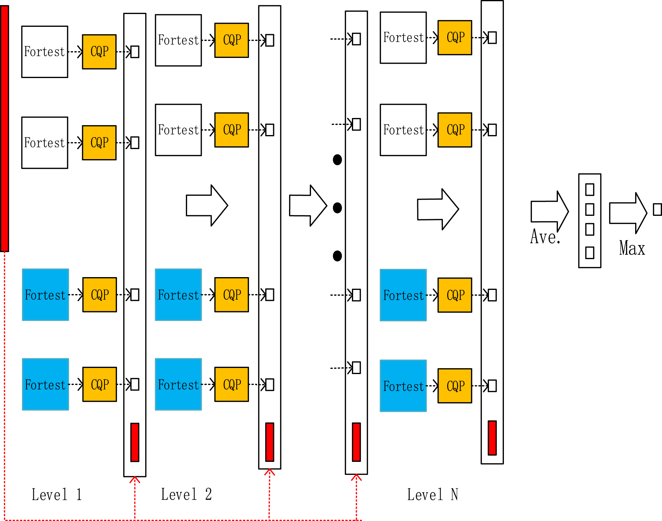
DeepForest-CQP Cascade Forest.

The upper and lower bound constrained CQP algorithm performs portfolio optimization in this paper. The multi-factor model emphasizes the breadth of the investment, so it is necessary to deny the weights of individual stocks with upper and lower bounds. The upper bound avoids assigning too much weight to a single store, thus increasing the risk. The lower bound is that the multi-factor model is a pure long portfolio, not a long-short model, so the lower bound constraint on the individual stock weights is 0, and the overall weight constraint is 1. Among them, the formula of the CQP algorithm in this paper is shown in (7). ${\begin{matrix} \underset{x}{Min} \frac{1}{2} x^{T} Hx + c^{T} x \\ s . t . {\begin{matrix} l ⩽ α^{T} x ⩽ b \\ Aeq \cdot x = beq \end{matrix} \end{matrix}$ (7)

In Equation (7), l, x, b, c, beq all are column vectors in R; Aeq, α denoted as coefficient matrix; H denoted as a semi-positive definite matrix.

The most crucial difference between these two types of forests lies in the candidate feature space; entirely random forests are split by randomly selecting $\sqrt{d}$ features in the entire feature space (d is the full features of the input), while ordinary random forests are divided by selecting separated nodes within a random feature subspace by Gini index [20]. The selected factors are combined, and each forest obtains input to the DeepForest-CQP algorithm and the predicted return of CSI 300. The CQP algorithm optimises to obtain the optimised stock prediction portfolio value Y = { y₁, y₂, . . . , y_n } . After passing to the next level, the validation set evaluates the prediction results of this cascade layer. If no performance improvement is found, it means that the model training to this cascade layer The training can be finished. Finally, based on all the results, the average value is taken and $\bar{Y} = {\bar{y_{1}}, \bar{y_{2}}, . . ., \bar{y_{n}}}$ is guaranteed to be the portfolio with the highest return of CSI 300 among stocks.

Also, to try to avoid the occurrence of overfitting, the class vectors generated by each forest are validated by k-fold crossover. Moreover, when a new cascade is generated, the performance of the entire cascade is estimated on the validation set, and the training process is terminated if there is no significant performance gain. Thus, the algorithmic model in the cascade is automatically determined by the algorithm and can be controlled adaptively so that the complexity of the model can be controlled and adapted to different size data sets. This is where the DeepForest-CQP algorithm differs significantly from other machine learning algorithmic models.

Since the information data carry out some kind of connection between the features that may affect, for example, in the image domain, there is a strong spatial relationship between the recognition location pixel points and a sequential relationship on the sequence data. It is inspired by this idea that DeepForest-CQP uses multi-grain scanning to enhance the cascade forest by using sliding windows of different sizes for data sampling, which in turn yields more information on feature subsamples and thus enables multi-grain scanning, the process of which is shown in Fig. 2.

Fig. 2

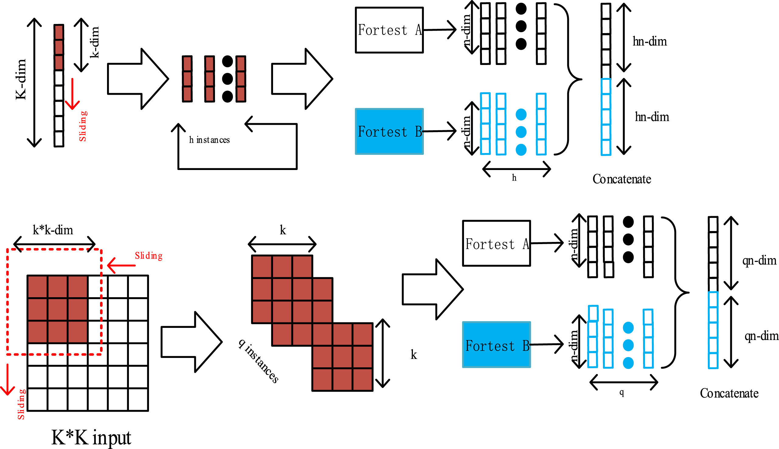
DeepForest-CQP MultiGrained Scanning.

4 Experiment and analysis

4.1 Data preprocessing

In general, the raw data are subject to data misalignment, missing values, extreme values, and different units and magnitudes of each influence factor, and there is no comparability between factors. To make the data fit the model better, missing values, data alignment, 3σ criterion, and Z-Score standardization are performed on the data.

After preprocessing the data, the positions are transferred at the beginning of each month, and the better stocks are selected based on the factor regressions and t-tests. When choosing the factors from the major categories, linear regression’s primary consideration of the backtest indicator is the annualized Sharpe ratio. The highest annualized Sharpe ratio in each class is selected as a priority.

Since there are more factors in the BP stock factor pool and more factors that perform better by linear regression, the screening was achieved by combining all other indicators. Subsequently, the factors screened by linear regression were subjected to a t-test. The primary selection criterion was |t|>2, and those that did not satisfy were excluded, Table 2 shows the final screening results.

Table 2
Factor feature screening results

Name of major category factor Factor name

Income Risk Category Factors ddncr, cmra12

Per share indicator type factor retained_earning_ps

Value-based factors ps, pb, pe

Growth factors sgro, net_profit_growth, ego, total_profit_growth

Technical indicator type factors cr20

Name of major category factor	Factor name
Income Risk Category Factors	ddncr, cmra12
Per share indicator type factor	retained_earning_ps
Value-based factors	ps, pb, pe
Growth factors	sgro, net_profit_growth, ego, total_profit_growth
Technical indicator type factors	cr20

The general orthogonalization methods are Schmidt orthogonalization, canonical orthogonalization and symmetric orthogonalization. Schmitt orthogonalization requires determining the orthogonal order of the factors, and if the orthogonal order is different, the final factors are also other; if the one-to-one correspondence between the factors before and after orthogonalization is to be maintained, the orthogonal order should be consistent and cannot change over time. The typical orthogonalization used for time series will have the problem of inconsistent correspondence between the factors before and after orthogonalization. Therefore, the symmetric orthogonalization method is used in this paper to deal with this problem. The symmetric orthogonalization of the orthogonal matrix C = E, due to the transition matrix $S = {UD}^{- \frac{1}{2}} U^{T} C$ , and finally the transition matrix $S = {UD}^{- \frac{1}{2}} U^{T}$ , is shown in Fig. 3.

Fig. 3

Symmetric orthogonalization of factors.

In this paper, we start the combination of the factors out of the sieve order. As shown in Fig. 4, the residual density distribution plot of its combined factors can offer a Gaussian distribution. Subsequently, we further observe the factor combinations in the form of scatter plots of residual distributions, as shown in Fig. 5. Figure 5 shows that although most of them fall within the interval, there are still some outside the falling interval, so there may be heteroskedasticity problems.

Fig. 4

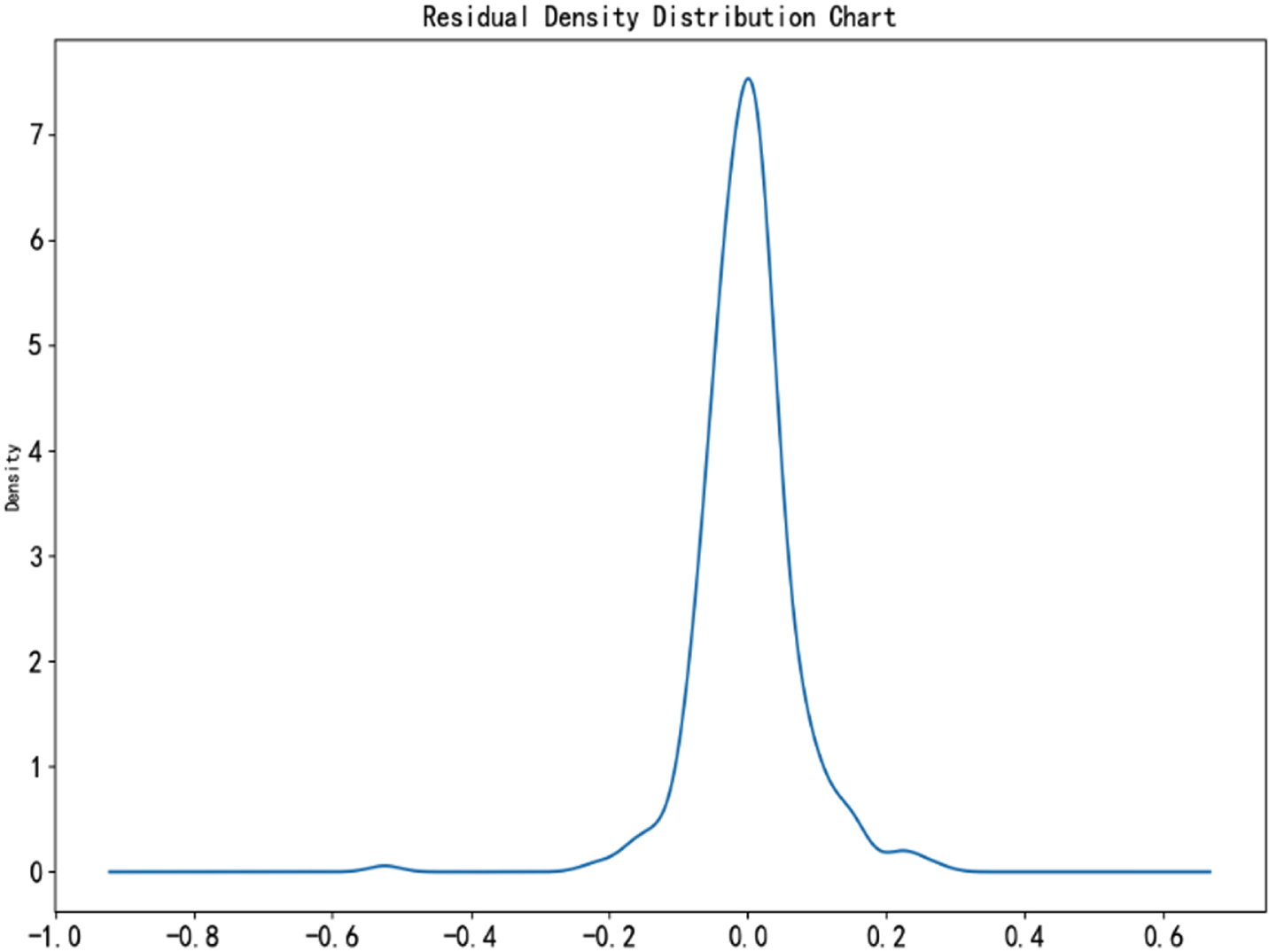
Residual density distribution chart.

Fig. 5

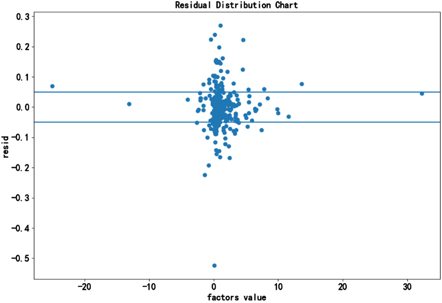
Residual distribution chart.

According to the problem shown in Fig. 5, it is necessary to perform a heteroskedasticity test on its combination factor. In this paper, according to Equations (6), the F statistic is calculated to be about 11.26; the LM statistic is about 106.87, the corresponding F statistic lookup table value is 2.68, and the corresponding cardinal value under the LM related degree of freedom is 36.12. It can be seen that both the F statistic and the LM statistic are more significant than the F statistic look-up table, and the corresponding cardinal value under the degree of freedom is substantial, rejecting the original hypothesis that there is heteroskedasticity.

In this paper, the treatment is based on the empirical validation in the Barra documentation manual [24], using the square root of the outstanding market value of individual stocks as weights in the weighted least multiplicative regression (WLS), which can eliminate the effect of heteroskedasticity in most of the intercept periods, as shown in Table 3, which removes the impact of heteroskedasticity on the subsequent prediction models.

Table 3

Heteroscedasticity treatment results

Before heteroskedasticity treatment		After heteroskedasticity treatment
F-statistic	LM statistic	F-statistic	LM statistic
11.26	106.87	2.16	31.44

4.2 DeepForest-CQP multi-factor model prediction

The selected factors are combined and processed as features into the DeepForest-CQP model for training and prediction; Fig. 6 shows in-sample prediction, and Fig. 7 shows out-of-sample prediction.

Fig. 6

DeepForest-CQP in sample prediction diagram.

Fig. 7

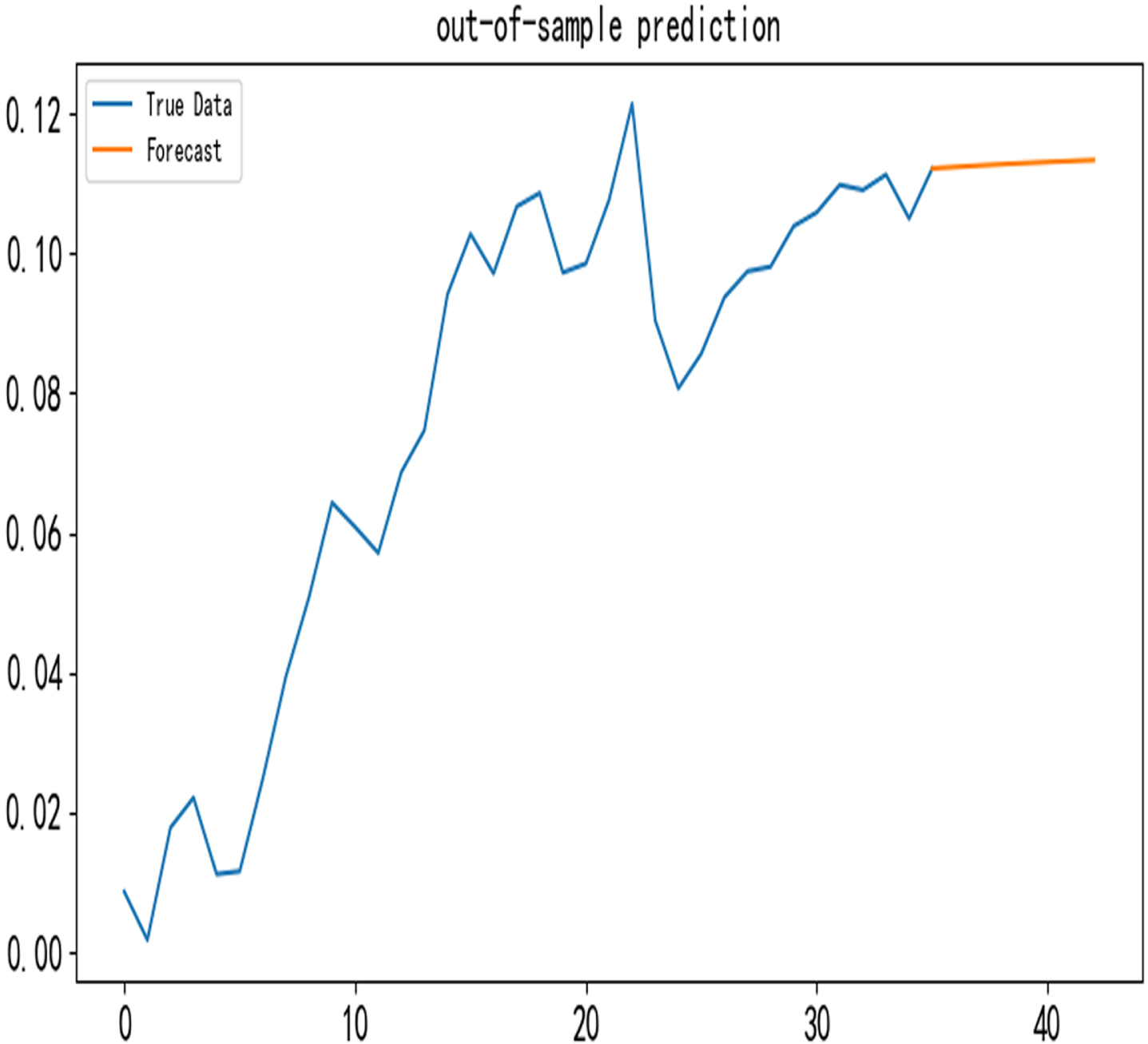
DeepForest-CQP out of sample prediction graph.

From Fig. 6, it can be seen that the DeepForest-CQP model fitted sequence trend has significant similarity with the real sequence trend, which means that it is a good fit. Also, to compare the DeepForest-CQP model with other machine learning models, the parameters of each machine learning model are set as in Table 4.

Table 4

Parameter settings for each machine learning model

Model	Parameter Setting
DeepForest-CQP	n_tree=80, n_bins = 255
Deep Forest	n_tree=80, n_bins = 255
RF	max_depth=5, n_estimators = 50, max_features=’log2’,learning_rate=0.01
LightGBM	objective=’binary’,max_depth=4,num_leaves=20,learning_rate=0.01
GBDT	n_estimators=200, max_depth = 8, loss=’ls’, learning_rate = 0.01
LSTM	hidden_size=64,num_layers=2,batch_first=True,dropout=0.2,LR=0.01, EPOCH=3, BATCH_SIZE=5

As shown in Table 5, it can be seen that the DeepForest-CQP model outperforms the other machine learning algorithm model metrics in all metrics. Also, it can be seen that the DeepForest-CQP model significantly improves each performance metric compared to the original Deep Forest model.

Table 5

Comparison of experimental model effects

Model	R2	MAE	RMSE
DeepForest-CQP	0.779	0.029	0.211
DeepForest	0.674	0.051	0.481
RF	0.481	0.117	0.923
LightGBM	0.596	0.071	0.718
GBDT	0.508	0.093	0.857
LSTM	0.578	0.080	0.801

4.3 Discussion

This paper better compares the performance of the DeepForest-CQP algorithm with other machine learning algorithms in the stock market. Also, to give professionals in all directions a clear understanding of the DeepForest-CQP multi-factor algorithm model in the stock market, the step of simulated trading is added in this paper. In the simulated trading, the DeepForest-CQP algorithm is compared with Deep Forest, GBDT, RF, LightGBM, and LSTM algorithms. In this way, the performance of various multi-factor algorithmic models in the stock market can be seen more intuitively and clearly to make a clear comparison.

The simulation trading period is from January 3, 2017, to February 28, 2020, with an initial capital of $10 million, and positions are transferred at the beginning of each month. The net value curves of simulated trades for each machine learning multi-factor model are shown in Figs. 8 13.

Fig. 8

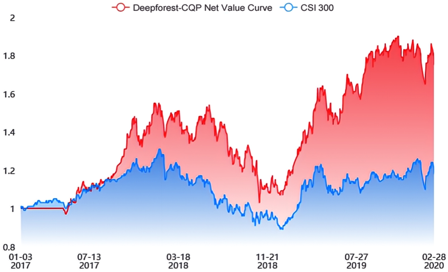
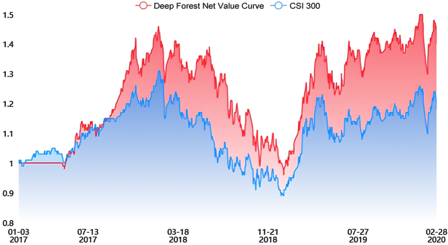
(a) Net curve of DeepForest-CQP multi-factor-model.

Fig. 8b

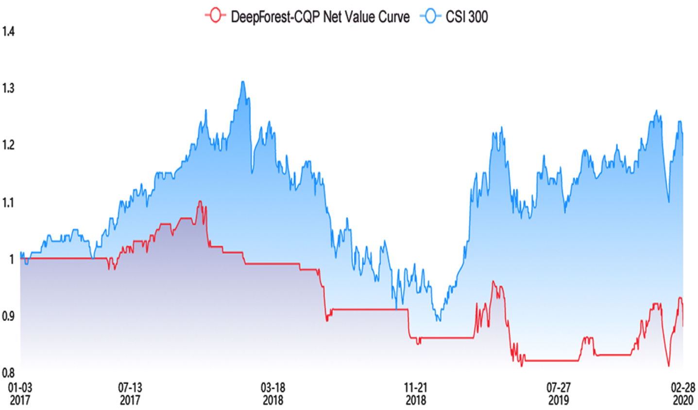
(b) Net curve of DeepForest-CQP multi-factor-model.

Fig. 9

Net curve of DeepForest multi-factor-model.

Fig. 10

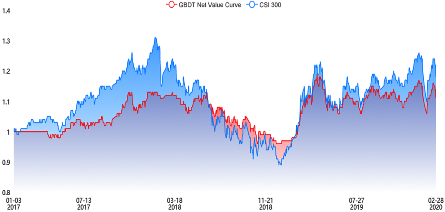
Net curve of GBDT multi-factor-model.

Fig. 11

Net curve of RF multi-factor-model.

Fig. 12

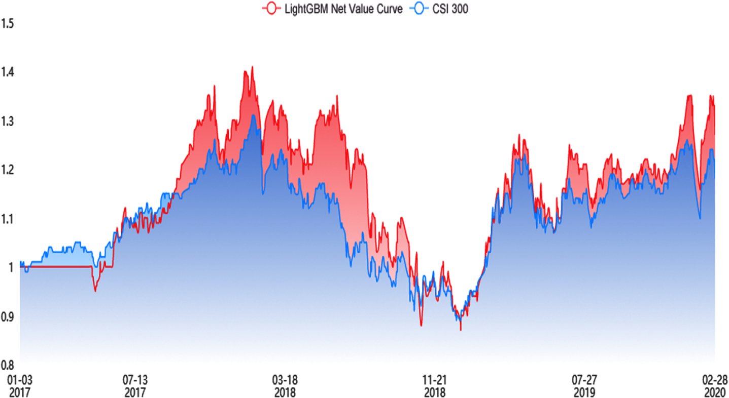
Net curve of LightGBM multi-factor-model.

Fig. 13

Net curve of LSTM multi-factor-model.

From Fig. 8(a), we can see that the net value curve of the DeepForest-CQP algorithm puts the curve of CSI 300 far above a lot, which shows that the DeepForest-CQP algorithm is the model that can obtain more robust excess returns and allow investors to gain income. While Fig. 8(b) is the result without feature selection, it can be seen that the net value curve is far below that of CSI 300, which can lead to enormous losses for investors.

As seen in Figs. 8(a) 9, the net curves of both the DeepForest-CQP multi-factor model and the Deep Forest multi-factor model place the CSI 300 curve well above. However, the DeepForest-CQP multi-factor model has a much higher net value curve than the Deep Forest multi-factor model, which shows that the DeepForest-CQP multi-factor model can achieve better excess returns than the Deep Forest multi-factor model.

As can be seen from Figs. 10 11, the GBDT multi-factor model and the RF multi-factor model net curves do not exceed the CSI 300 curve. This indicates that these two models do not have significant effects in CSI 300.

Figures 10 through 11 show that the net curves of the LightGBM multi-factor model and the LSTM multi-factor model can, most of the time, exceed the CSI 300 curve. This also indicates that some gains can be obtained, but not as much as those obtained by the DeepForest-CQP multifactor model.

To further observe the performance of DeepForest-CQP in the stock market, not only from the backtest return performance graph but also the Deep Forest, GBDT, LightGBM, RF, and LSTM multi-factor model backtest metrics should be compared, as shown in Table 6.

Table 6

Comparison of experimental model backtest metrics.

Model	AR	α	β	Sharpe ratio	Maximum retracement rate	Accumulated earnings
DeepForest-CQP	30.18%	0.38	1.88	0.81	10.47%	145.85%
DeepForest	14.68%	0.13	1.04	0.58	30.01%	78.54%
RF	2.54%	–0.02	0.69	0.31	31.11%	10.52%
LightGBM	7.12%	0.06	0.71	0.46	38.04%	30.48%
GBDT	3.52%	–0.01	0.96	0.35	24.96%	7.15%
LSTM	6.32%	0.05	0.81	0.41	27.12%	25.19%

5 Conclusion

From the experimental process and final results, it is a proven methodological model to design a corresponding portfolio strategy by selecting influential factors through multi-factor quantitative stock selection to obtain stable returns.

In this study, the DeepForest-CQP multi-factor stock selection model is compared with Deep Forest, GDBT, LightGBM, RF, and LSTM multi-factor models, and the factor data are processed and examined in detail. The factor combinations are used as inputs to the algorithm for prediction, and the projections are automatically combined. In addition, simulated trades are used to verify that the DeepForest-CQP multi-factor model has more significant superiority over other machine learning models and is a model that can achieve relatively robust returns for investors. Future expansions will focus on the following two areas:

Because the BP factor library divides its factors into twelve categories, we can only select the existing ones from the limitation of our knowledge. However, in real life, stocks are affected by many factors, and this thesis cannot cover all of them, so we can further broaden the factors and dig for new factor information in the subsequent research.

The model is improved and optimized with the CQP algorithm to achieve risk control in this paper. In the subsequent study, other methods can be used for optimization to achieve better results.

Credit authorship contribution statement

Chen Tang: Conceptualization, Methodology, Software, Formal analysis, Investigation, Data Curation, Writing –Original Draft, Visualization. Qiancheng Yu: Writing –Review & Editing, Supervision. Xiaoning Li: Supervision. Zekun Lu: Supervision. Yufan Yang: Supervision.

Funding

This work was supported by the Doctoral Program of Northern MinZu University (Grant No. 2020KYQD48); The 2022 University Research Platform “Digital Agriculture Empowering Ningxia Rural Revitalization Innovation Team” of Northern University for Nationalities (2022PT_S10); The National Natural Science Foundation of China (Grant No. 62062001); The major key project of school-enterprise joint innovation in Yinchuan 2022 (2022XQZD009) and the innovation project of North Minzu University (YCX21097).

Declarations

Conflict of interest The authors declared that they have no conflicts of interest in this work.

Footnotes

Acknowledgments

The authors did not receive support from any organization for the submitted work.

References

Petkova

, Do the Fama-Frech factors proxy for innovations in predictive variables, The Journal of Finance 61(2) (2006), 581–612.

Sun

, Muliti-Factor Quantitative Investment Strategy and Empirical Analysis, Nanjing University, 2016.

Pei

D.W.

, Method of multiple-factor stock price predictions with deep learning, University Of Science And Technology of China, 2019.

Song

, One of the Multi-factor Graduate Models: Single Factor Testing.Bohai Securities Co, Ltd, 2017.

Shi

, Hu

, Mo

, et al., Attention-based CNN-LSTM and XGBoost hybrid model for stock prediction, arXiv e-prints, 2022.

Agrawal

, Shukla

P.K.

, Nair

, et al., Stock Prediction Based on Technical Indicators Using Deep Learning Model, Computers, Materials & Continua (1) (2022), 18.

Cheng

M.F.

and Gao

S.P.

, Multi-Scale Stock Prediction Based on Deep Transfer Learning, Computer Engineering and Applications 58(12) (2022), 249–259.

Zhuang

X.N.

, Chen

Z.Y.

, Wu

Y.C.

, et al., Quantum Quantitative Trading: High-Frequency Statistical Arbitrage Algorithm, 2021.

S.Z.

, Research on quantitative trading strategy based on EMD algorithm, Economic Research Guide (19) (2019), 101–104.

10.

Cen

Y.F.

, Zhang

C.G.

, Cen

and Zhao

, A stock price prediction method based on proximal reinforcement learning, Control and Decision Making 36(04) (2021), 967–973. DOI: 10.13195/j.kzyjc.2019.1245

11.

Mitchell

T.M.

, Machine Learning. New York: McGrawHill, 1997.

12.

Liu

, He

, Gao

W.Q.

, Fu

X.W.

and Kang

X.M.

, Alteroscedasticity test for a partial linear EV model under the absence of response variables, Applied Probabilistic Statistics (37) (2021), 346–360.

13.

Breusch

T.S.

and Pagan

A.R.

, A Simple Test for Heteroscedasticity and Random Coefficient Variation, Econometrica 47(5) (1979), 1287–1294.

14.

Zhou

Z.H.

and Feng

, Deep forest: Towards an alternative to deep neural networks, arXiv:170 2.08835, 2017.

15.

Zhou Zhihua and Feng

, Deep forest: towards an alternative to deep neural networks, International Joint Conference on Artificial Intelligence, 2017.

16.

Zhu

X.Y.

, Yan

Y.Y.

and Liu

Y.A.

, Flame Detection Based on Deep Forest Model, Computer Engineering (7) (2018), 264–270.

17.

Liu

, Wu

and Zheng

Y.C.

, Classification of Cancer Based on Deep Forest and DNA Methylation, Computer Engineering and Applications 56(13) (2020), 189–193.

18.

Gong

Z.H.

and Wang

J.N.

, A Weighted Deep Forest Algo-Rithm, Computer Applications and Software (2) (2019), 274–278.

19.

Danelljan

, Robinson

, Khan

F.S.

, et al., Beyond correlation filters: learning continuous convolution operators for visual tracking, Proceedings of the 2016 European Conference on Computer Vision, Berlin:Springer 2016 (2016), 472–488.

20.

Menchero

, Orr

, Wang

. The Barra US equity model (USE4), methodology notes, English, MSCI (May, 2011).