Bi-LSTM fault diagnosis method for rolling bearings based on segmented interception AR spectrum analysis and information fusion

Abstract

The rolling bearing fault diagnosis is affected by industrial environmental noise and other factors, leading to the existence of some redundant components after signal decomposition. At the same time, the existence of the modal aliasing phenomenon in empirical mode decomposition (EMD) and the relevant improved algorithms also leads to the existence of many invalid features in the components. These phenomena have great influence on the bearing fault diagnosis. So a rolling bearing bidirectional-long short term memory (Bi-LSTM) fault diagnosis method was proposed based on segmented interception auto regressive (SIAR) spectrum analysis and information fusion. The ensemble empirical mode decomposition (EEMD), the complementary ensemble empirical mode decomposition (CEEMD) and the robust EMD (REMD) algorithms decompose the rolling bearing fault signals, and AR spectrum analysis is performed on the obtained components respectively. By comparing the AR spectra of the components corresponding to different fault locations, the effective AR spectral values are intercepted as the eigenvalues of the data, and finally all the eigenvalues are fused to achieve the purpose of screening effective features more efficiently so as to reduce the impact of feature redundancy caused by mode aliasing on neural network training. Then the Bi-LSTM neural network was used as a rolling bearing fault diagnosis classifier, and the simulation experiments were conducted based on the rolling bearing fault signal data from Case Western Reserve University to verify the effectiveness of the proposed feature extraction and fault diagnosis method.

Keywords

Rolling bearing fault diagnosis AR spectrum analysis information fusion empirical mode decomposition LSTM

1 Introduction

As an indispensable part of the industrial production equipment, the rolling bearing mainly exists in extremely harsh working conditions, including high speed, heavy load and the strong impact of the environment, temperature, wind, water spray and other external physical and chemical erosion. Any unexpected mistakes will result in failure of mechanical system. In common rotating machinery, rolling bearing faults account for one-third. Therefore, fault diagnosis of bearings can effectively prevent the serious consequences caused by bearing faults, which is of great practical significance [1]. The fault diagnosis methods of rolling bearings can be divided into two categories: establishing normal state model and analyzing vibration data. The establishment of the normal state model requires higher requirements on its working environment. A slightly unstable environment will affect the uniqueness of the normal model, while the working environment of bearings is greatly affected by uncontrollable factors such as noise, so this method is difficult and not operable enough. As the vibration signals of bearings contain a large amount of fault feature information, the current bearing fault diagnosis is mainly based on the processing of vibration signals. So how to extract effective fault features from vibration signals has become a key issue, which is related to the effect of bearing fault diagnosis [2].

The empirical mode decomposition algorithm proposed by Huang et al. is adaptive to decompose non-stationary and nonlinear fault signals into several eigenmode components, and each component has a specific physical meaning. Therefore, this method is widely used in the field of fault diagnosis. However, it also has some limitation. For example, windowing effect of Hilbert transform leads to errors at both ends of the modulation signal, marginal spectrum peak overlaps, and it is difficult to distinguish fault features and other problems. On this basis, many scholars have improved it so as to make up for the shortcomings of EMD algorithm. Ref. [3] analyzes the boundary problems of EMD decomposition through cosine window function, and the conclusion proves that the fault features contained in each modal component have different influences on the diagnosis effect. In Ref. [4], Hilbert-Huang transform was used to analyze the original fault signals to extract fault features, and support vector machine (SVM) was used to verify the classifier effect, thus achieving fault diagnosis. Ref. [5] improved EMD method through multi-objective optimization so as to extract the rolling bearing fault features for fault identification and classification. But the above fault diagnosis methods have different degrees of modal aliasing phenomenon, that is, a component contained in the failure data of the characteristics of multiple scales, or at the same time scale characteristics are broken down into different components. So the modal aliasing phenomenon will increase the difficulty of fault feature extraction, and have great negative impact on bearing fault diagnosis.

Ensemble empirical mode decomposition was proposed on the basis of EMD, which is a signal analysis method assisted by white noise. The mode aliasing in EMD is avoided by adding Gaussian white noise into the original signal. In recent years, many scholars have applied EEMD and its improved algorithm to the field of mechanical fault diagnosis. Ref. [6] integrates EEMD and optimized support vector regression model to diagnose the fault location of piston pump. In literature Ref. [7], EEMD, correlation coefficient and Hilbert-Huang were used to extract fault features of bearings, and the final experiment showed that this method could effectively solve the mode mixing effect of EMD. The CEEMD was proposed by adding a pair of opposite white noises into the signal to be analyzed [8]. Thus, the decomposition error caused by white noises is reduced, the number of noise sets is reduced, and the computational efficiency is improved. Ref. [9] uses CEEMD to decompose original signals, and proposes a new method to eliminate intrinsic mode function (IMF) components with defective information. The signal is then reconstructed from the sum of the relevant IMF, and the frequency-weighted energy operator is adjusted to extract the amplitude and frequency modulation from the selected IMF. In Ref. [10], EMD decomposition and AR spectrum estimation are combined to be used in the gearbox fault diagnosis. AR spectra of the previous six IMF components of signals in different states were compared, and then EMD-AR spectrum energy eigenvalues were extracted, and the eigenvalues were input into the constructed SVM classifier. The results show that the method can be effectively applied to gearbox fault diagnosis of special vehicles, and the diagnostic accuracy reaches 94.5%. Ref. [11] proposed a new method of combined photovariation period analysis based on EMD-AR spectrum. Firstly, the observed data were decomposed by EMD to obtain the various modal components, and the correlation coefficients between them and the original optical variation curve were calculated. Then, the AR spectrum was estimated by summing up the components with high correlation. Finally, the periodic analysis method of the power spectrum was applied to the optical variation data analysis of celestial bodies. Ref. [12] proposed a fault feature signal analysis method based on the combination of variational modal decomposition (VMD) and AR spectrum. The results show that the fault feature extraction method based on VMD-AR spectrum solves the problem of selecting decomposition mode number and avoids its empirical selection. Although the diagnosis methods proposed in the above literature can suppress the mode aliasing phenomenon to a certain extent, single signal decomposition algorithm is easy to cause signal feature loss and have a great influence on the diagnosis results.

In view of the shortcomings of the above methods, in recent years, many scholars have introduced the means of information fusion into mechanical fault feature extraction, and achieved good results. Ref. [13] presents a method for device fault diagnosis based on failure rate and failure symptoms. Firstly, an algorithm for calculating equipment failure rate was proposed based on Weibull distribution model. Then the probability of failure is evaluated according to the failure phenomenon and a fault diagnosis model based on failure rate and failure symptoms was realized/ Finally, its effectiveness was verified through calculation examples. This method comprehensively considers the failure rate, failure mechanism, failure symptoms, and the acquisition difficulty of failure symptoms, and greatly improves the accuracy of fault diagnosis. Ref. [14] combined with the robustness of deep convolutional neural networks and the characteristics of vibration signals, introduced information fusion technology to enhance the feature representation ability and portability of the diagnostic model. Based on the multi-sensor and narrowband decomposition techniques, a fusion cell convolution structure was proposed to extract multi-scale features from different sensors. It was tested on two data sets. Compared with some existing works, the proposed method had higher generalization ability, which proved the effectiveness of the proposed fusion unit for feature extraction on both source and target tasks.

In this paper, based on different EMD varients, combined with the AR spectrum analysis of modal components and the analysis of AR spectra, the effective frequency band of the intercept value of AR spectrum was selected as the fault characteristic parameter so as to reduce the invalid and redundant features and the influence of mode aliasing on neural network training. A method of information fusion and dimension reduction was proposed, that is, 10 AR spectral values are intercepted as feature parameters by EEMD, CEEMD and REMD algorithms and AR spectral analysis respectively. Then a 30-dimensional feature vector was obtained by concatenating them together, and the top 20 feature values with variance values were screened by low variance. Finally, Pearson correlation coefficient was used to select 10 characteristic parameters with large correlation coefficients as the final characteristic values, and the obtained characteristic values were input into BI-LSTM neural network classifier to verify the effectiveness of the proposed fault diagnosis method. The simulation results show that this method has a better bearing fault diagnosis effect.

2 Basic principle of AR spectrum estimation

AR model is a commonly used time sequence estimation and analysis method, which has the advantages of high resolution and correct positioning, and can effectively overcome the windowing effect of signals [10 –12]. The stochastic process can be expressed as: $X_{(n)} = \sum_{i = 1}^{k} a_{i} s (n - 1) + u (n)$ (1) where, n is the discrete data point, a_i (i = 1, 2, 3, . . . . k) is the AR model coefficient, i is the serial number of each coefficient, k is the maximum of the serial number of the coefficient, and u (n) is a white noise sequence whose variance δ². Yule-walker method was used to solve the coefficient of AR model, and the Akaike information criterion (AIC) was used as the commonly used order criterion for the AR model. The AR power spectrum estimation is calculated by: $P (e^{j ω}) = \frac{δ^{2}}{{| 1 + \sum_{i = 1}^{p} a_{i} e -^{j ω i} |}^{2}}$ (2) where, j is an imaginary unit and ω is an angular variable. The above two formulas are autoregressive models, referred to as AR models. The obtained power spectrum estimation is called AR spectrum. The first k + 1 autocorrelation function X_(n) is obtained, and the power spectrum of X_(n) can be obtained by substituting it into Equation (2).

3 Fault signal analysis of rolling bearing based on segmented AR spectrum estimation

3.1 Rolling bearing fault diagnosis signal analysis based on EEMD-AR

3.1.1 Basic principles of EEMD algorithm

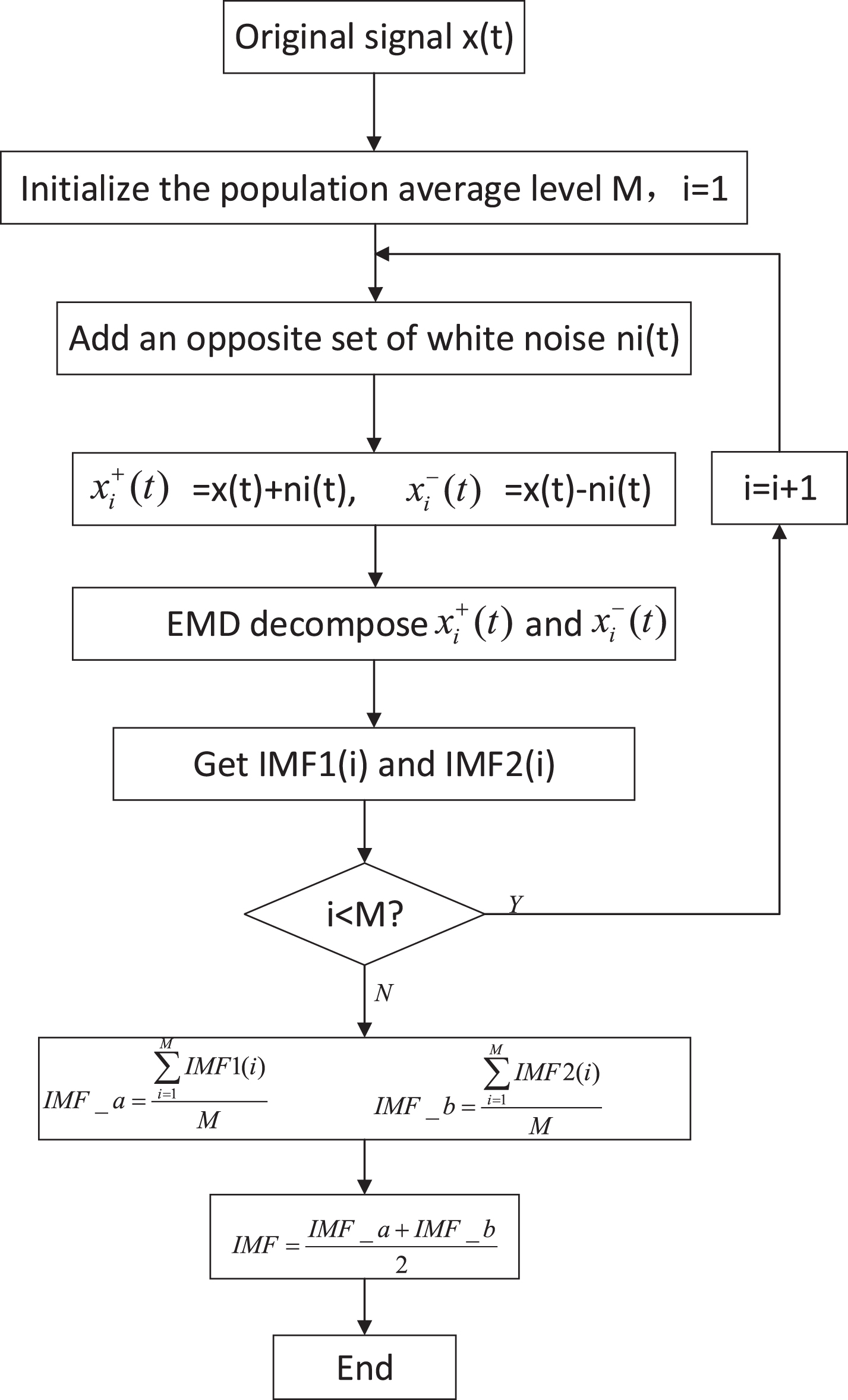
The EEMD decomposition method mainly adds white noise into the signal according to the characteristic so that the mean value of white noise is zero. In essence, it is an improvement of EMD algorithm, whose core is still the EMD decomposition. Average processing is carried out for the decomposition results. The more times of average processing, the less influence noise brings to the decomposition results, thus inhibiting the influence of mode aliasing. The main decomposition steps are described as follows [15].

Add the random white noise n_i (t) with a certain amplitude to signal x (t) so as to form a new set of signal x_i (t). $x_{i} (t) = x (t) + n_{i} (t) \begin{matrix} i = 1, 2, . . ., M \end{matrix}$ (3)

The EMD decomposition of x_i (t) is performed to obtain the IMF component.

The final IMF component is obtained by averaging the obtained IMF components.

3.1.2 EEMD-AR effective frequency band experiment and analysis

In order to obtain the frequency band of effective AR spectrum value after decomposition of EEMD algorithm and AR spectrum analysis of its components, the following simulation experiments are designed for analysis. Two groups of fault data were selected for analysis. The diagnosis objects were the faults of the inner ring, outer ring and rolling body of the rolling bearing. In order to simulate the early bearing faults, fault data with damage diameter of 0.007 mm were selected for verification. Experimental data information is listed in Table 1 [16].

Table 1
EEMD-AR analysis experimental data information

Data group category Single sample data points Damage to the diameter Failure position Category

Data 1 1000 0.007 mm Inner ring fault 1

Outer ring fault 2

Rolling body faul 3

Normal 4

Data 2 1000 0.007 mm Inner ring fault 1

Outer ring fault 2

Rolling body faul 3

Normal 4

Data group category	Single sample data points	Damage to the diameter	Failure position	Category
Data 1	1000	0.007 mm	Inner ring fault	1
			Outer ring fault	2
			Rolling body faul	3
			Normal	4
Data 2	1000	0.007 mm	Inner ring fault	1
			Outer ring fault	2
			Rolling body faul	3
			Normal	4

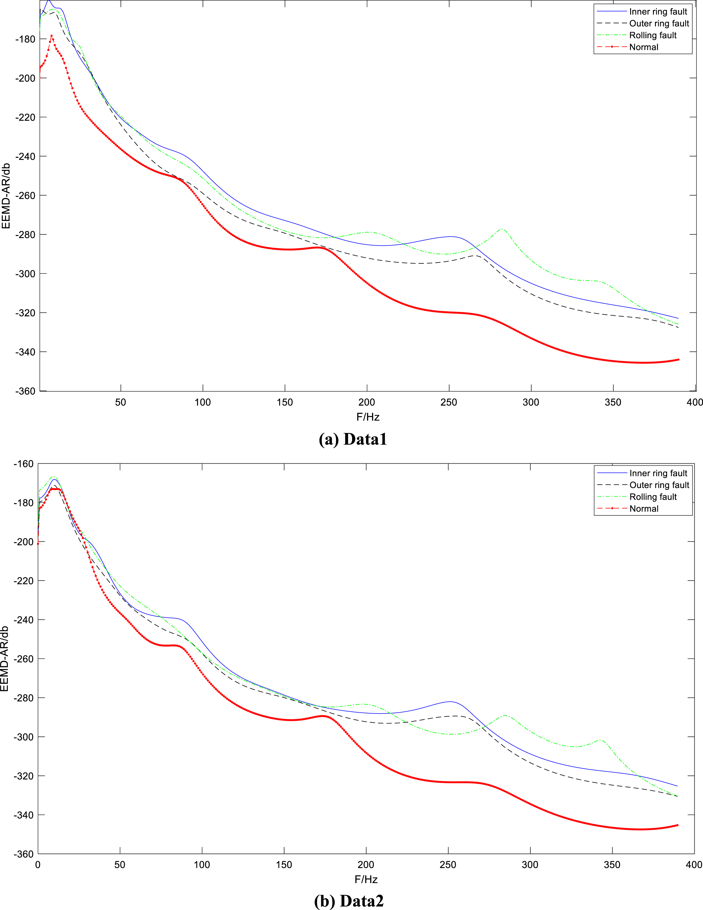
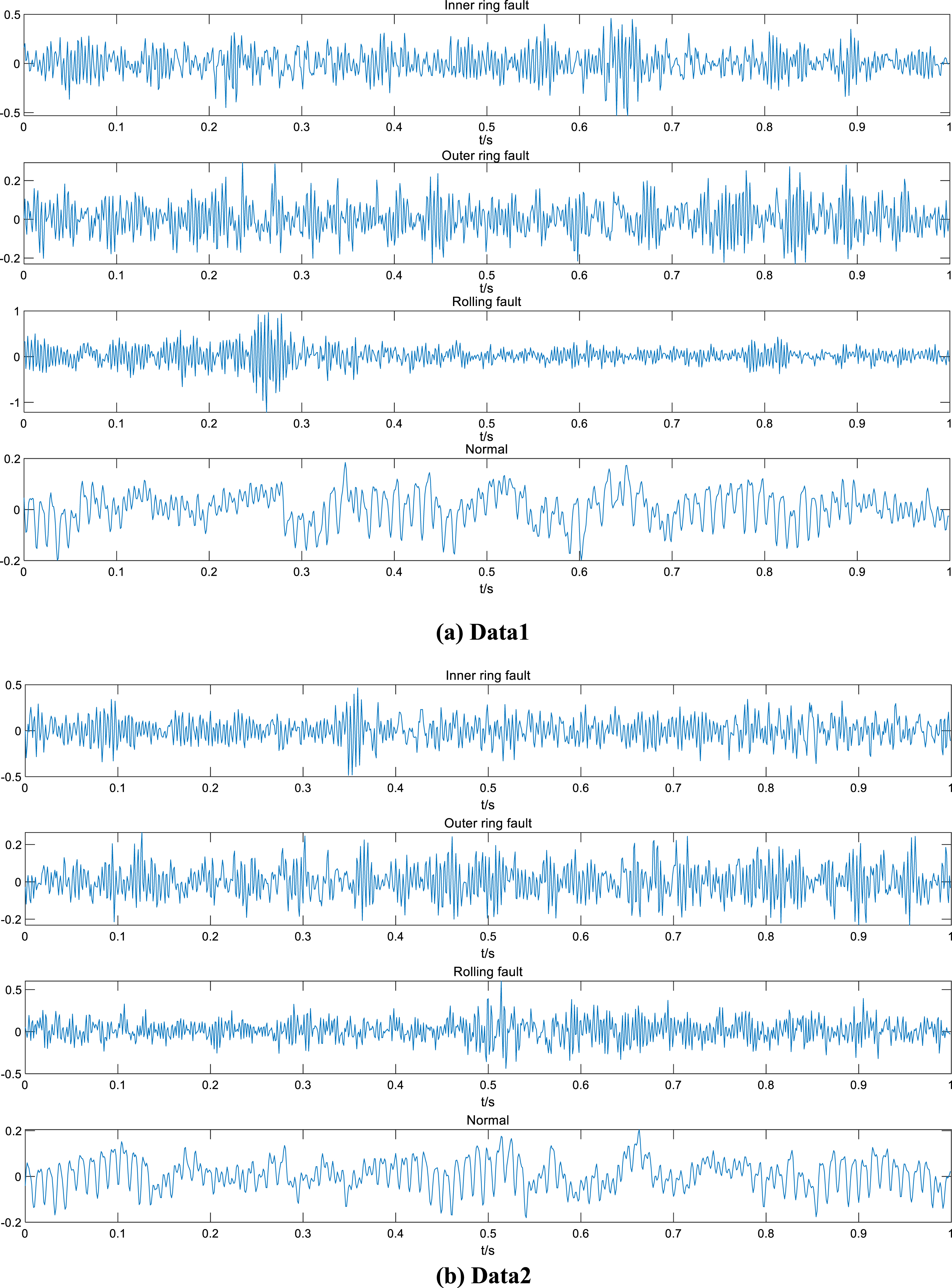
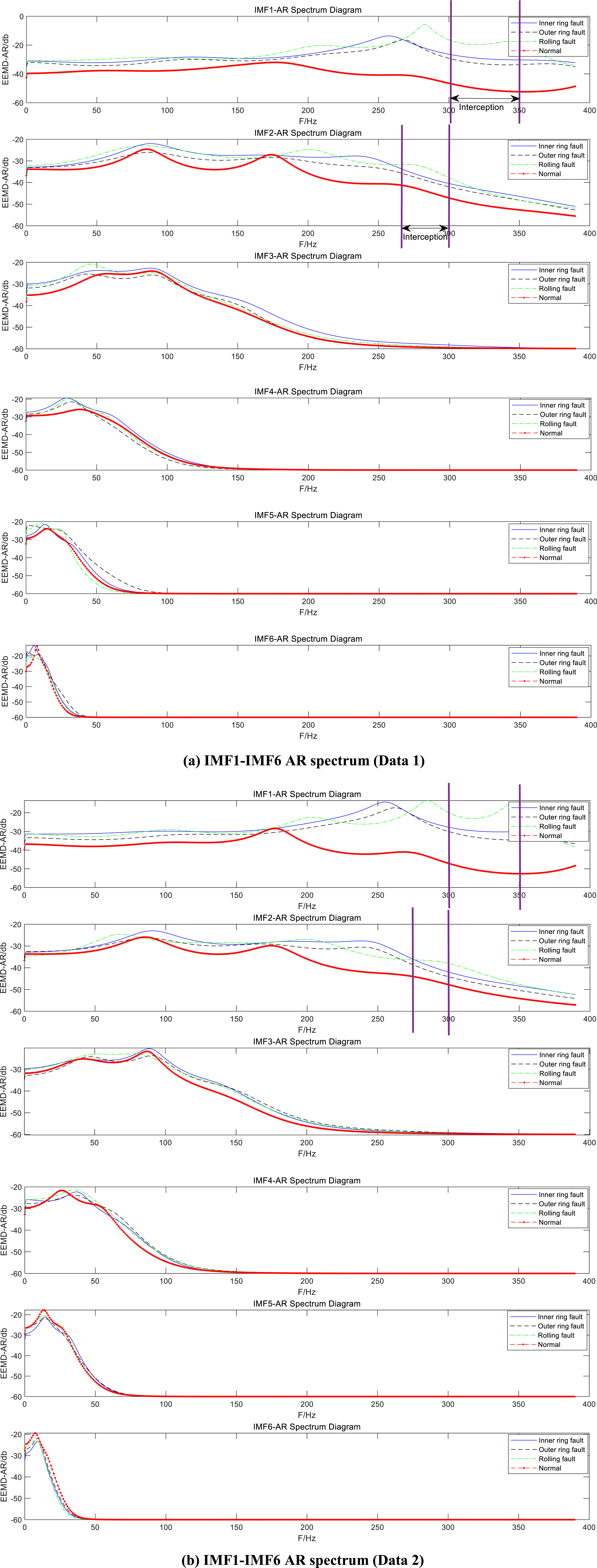
AR spectrum analysis was performed on the previous six IMF components with a large energy ratio which were decomposed by EEMD algorithm to obtain the AR spectrum. Figures 1 –3 shows the simulation diagram of EEMD-AR analysis experiments. Figure 1(a) shows the AR spectra of the six IMF components of data 1, and Fig. 1(b) shows the AR spectra of the six IMF components of data 2. It can be analyzed from Fig. 1 that the first three IMF components of the two groups of data have extremely same variation trend, and the AR spectrum range in the corresponding frequency band is almost the same. Among them, the AR spectrum values of IMF1 and IMF2 are in the frequency band of 300–350 Hz, the AR spectrum values of each fault part of IMF3 are in the frequency band of 200–250 Hz, and there is an obvious gap between them. On the other hand, the AR spectrum values of these frequency bands are rolling body fault, inner ring fault, outer ring fault and normal data respectively from top to bottom, which are considered as valid features. Compared with other frequency bands, such as IMF1 in frequency band 150 to 200, the AR curves of inner ring fault and rolling body fault are very close, and even overlap. These eigenvalues are considered as invalid features, which will affect the training of neural network and reduce the accuracy of fault identification, so they should be eliminated. In the AR spectrum of the latter three IMF components shown in Fig. 1, almost all of the frequency bands in AR curves are very close between at least two fault parts, so these components are not directly considered. Figure 2 is the sum of AR spectra of the previous six IMF components. It can be seen from Fig. 2 that the AR spectral values of each fault part have the largest difference interval in frequency band 200–250 Hz and 300–350 Hz [17, 18]. Figure 3 shows the time-domain waveform of fault data.

Fig. 1

AR spectra of the previous six IMF components decomposed by EEMD.

Fig. 2

Sum of AR spectra of the previous six IMF components.

Fig. 3

Time-domain waveform of fault data.

3.1.3 EEMD-AR fault feature extraction

The captured specific frequencies of AR spectral analysis are set as the fault signal characteristic value. In that the interception of band is longer, the characteristics of the reference number is larger, so it can not directly be used for neural network training. There will be a great feature vector dimensions caused by excessive training hard, which will ultimately affect the accuracy of the fault recognition [19]. Therefore, dimension reduction must be performed on the intercepted fault characteristic values. In this part, the mean-low variance filtering is used to reduce the dimension of feature vector. Figure 4 is the flowchart of the EEMD algorithm to extract the characteristics and obtain a larger dimension vector. After obtaining a feature vector with a large dimension according to this process, the average value of the feature values is firstly got based on all the feature numbers in the data set according to the fault category, and a data set matrix with 4 rows and N columns is got (N is the number of feature values of a single sample). Then calculate the square difference of each column of elements, filter out the features with lower variance value ranking, and select the top 10 features as the final feature parameters. Figure 7 is the sum of AR spectra of the previous six IMF components. It can be seen from Fig. 7 that the AR spectral values of each fault part have the largest difference interval in frequency band 275–350 Hz. Figure 8 shows the time-domain waveform of fault data.

Fig. 4

Flow chart of feature extraction for EEMD-SIAR analysis.

Fig. 7

Sum of AR spectra of the previous six IMF components.

Fig. 8

Time-domain waveform of fault data.

3.2 Rolling bearing fault diagnosis signal analysis based on CEEMD-AR

3.2.1 Basic principles of CEEMD algorithm

CEEMD algorithm improves EEMD algorithm by adding the N opposite noise signs into the signal and carrying out the EMD decomposition so as to finally obtain the final IMF component after 2 N averaging. CEEMD decomposition process is shown in Fig. 5 and the detailed decomposition process is described as follows [20].

Fig. 5

CEEMD decomposition flow chart.

A group of white noise signals with negative numbers are included in the original data to form a group of new signals: $x_{i}^{+} (t) = x (t) + n_{i}^{+} (t)$ (4)

$x_{i}^{-} (t) = x (t) + n_{i}^{-} (t) i = 1, 2, 3 . . . . . ., M$ (5) where, x (t) is the original signal, $n_{i}^{+} (t)$ is the positive noise, and $n_{i}^{-} (t)$ is the negative noise.

EMD decomposition of $x_{i}^{+} (t)$ and $x_{i}^{-} (t)$ was performed to obtain the IMF components and IMF1 and IMF2 were obtained by means processing.

The final decomposition result IMF is obtained by averaging IMF1 and IMF2.

3.2.2 CEEMD-AR effective frequency band experiment and analysis

Similar to the above EEMD-AR analysis, the following experiments are designed to analyze the effective frequency range of fault data. The experimental data information is shown in Table 1. Figures 6 –8 shows the simulation diagram of CEEMD-AR analysis experiments. Figure 6 shows the AR spectra of the first three IMF components. Figure 6(a) shows the AR spectra of the six IMF components in data 1, and Fig. 6(b) shows the AR spectra of the six IMF components in data 2. According to the AR spectra of the previous three IMF components in Fig. 6, two groups of data have extremely same changing trend, and the AR spectrum range in the corresponding frequency band is almost the same. Among them, the AR spectrum values of IMF1 and IMF2 in the frequency band 300–350 Hz and 275HZ to 300HZ respectively have an obvious gap between the AR spectrum values of each fault part, and these parts of the spectrum values are considered as valid fault features. Compared with other frequency bands, such as IMF1 in frequency band 150 to 200 and IMF3 in all frequency bands, the AR curves of inner ring faults and outer ring faults are very close, and even overlap. These eigenvalues are considered as invalid features, which will affect the training of neural network and reduce the accuracy rate of fault identification, and should be eliminated. In the AR spectra of the last three IMF components in Fig. 6, AR curves of at least two fault parts are very close to each other in almost all frequency bands, which is close to coincidence. Therefore, these components are not directly considered.

Fig. 6

AR spectra of the previous six IMF components based on of CEEMD decomposition.

3.2.3 CEEMD-AR fault feature extraction

Its feature extraction process is similar to that of EEMD. The feature extraction process of CEEMD-SIAR analysis is shown in Fig. 9.

Fig. 9

Feature extraction flow chart of CEEMD-SIAR analysis.

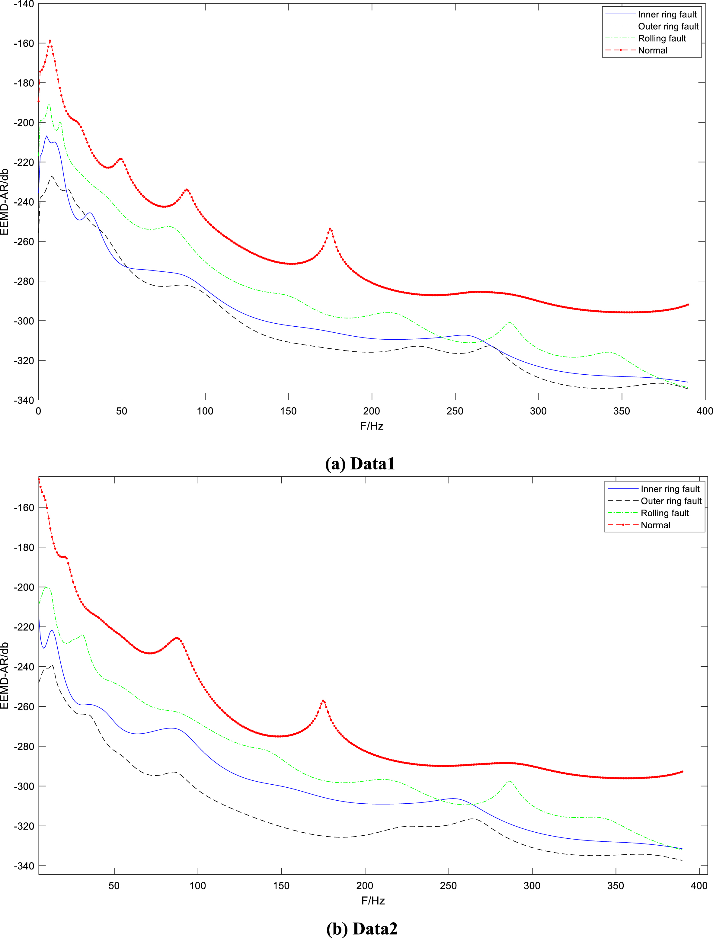
3.3 Rolling bearing fault diagnosis signal analysis based on REMD-AR

REMD is an improved empirical pattern decomposition, which is supported by the soft screen stop criteria (SSSC). SSSC is an adaptive screening stop standard used to automatically stop the screening process of EMD [21, 22]. It extracts a set of single-component signals (called intrinsic mode functions) from the mixed signals. It can be used with Hilbert transform or other demodulation techniques for time-frequency analysis. Similar to the above EEMD/CEEMD-AR analysis, the following experiments are designed to analyze the effective frequency range of fault data. The experimental data information is shown in Table 1. Figures 10 –12 show the simulation diagram of REMD-AR analysis experiments. Figure 10(a) is the AR spectrum of the six IMF components of data 1, and Fig. 10(b) is the AR spectrum of the six IMF components of data 2. According to the AR spectra of the first three IMF components in Fig. 10, two sets of data have extremely same changing trend, and the AR spectrum range in the corresponding frequency band is almost the same.

Fig. 10

AR spectra of the previous six IMF components decomposed by REMD.

Fig. 11

Sum of AR spectra of the previous six IMF components.

Fig. 12

Time-domain waveform of fault data.

Among them, the AR spectrum values of IMF1, IMF2 and IMF3 in the frequency band of 300–350 Hz, 130HZ to 170HZ and 75–100 Hz respectively have obvious gap between the AR spectrum values of each fault part, and these parts of the spectrum values are considered as valid fault features. Compared with other frequency bands, AR curves of inner and outer ring faults and rolling body faults of IMF1 in frequency band 220 to 270HZ are very close to each other, and even coincide with each other. These eigenvalues are considered as invalid features, which will affect the training of neural network and reduce the accuracy rate of fault identification, which should be eliminated. In Fig. 10, AR spectra of the last three IMF components in almost all frequency bands have AR curves that are very close to or close to overlap between at least two fault parts, so these components are not directly considered. Figure 11 is the sum of AR spectra of the previous six IMF components. It can be seen from Fig. 11 that the AR spectral values of each fault part have the largest difference interval in frequency band 300–350 Hz, 130HZ to 170HZ, and 75 to 100HZ. Figure 12 shows the time domain waveform of fault data, and Fig. 13 shows the REMD feature extraction process.

Fig. 13

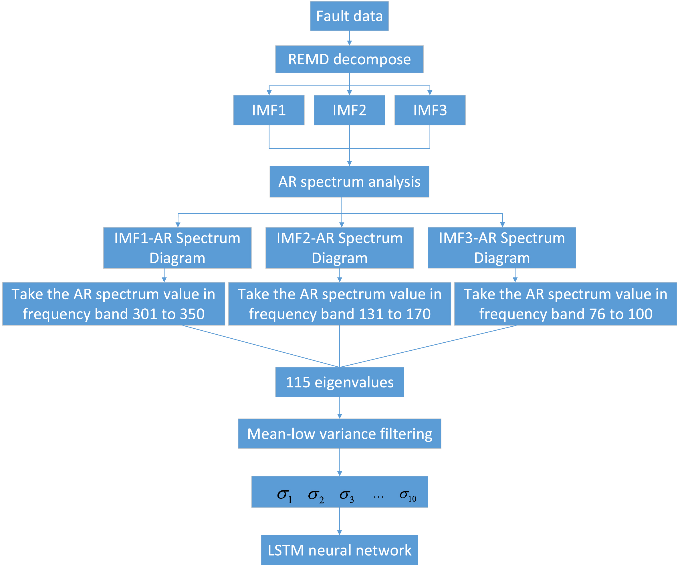
Feature extraction flow chart of REMD-SIAR analysis.

4. Bi-LSTM fault diagnosis method for rolling bearings based on segmented AR spectrum analysis and information fusion

4.1 Rolling bearing fault diagnosis method based on SIAR and information fusion

Finally, as shown in Fig. 14, the 10 characteristic parameters obtained by three algorithms in accordance with the above process are fused to obtain 30-dimensional characteristic parameters. Then, the first 20 characteristic values of variance are screened through low variance. Finally, 10 characteristic parameters with large correlation coefficients are selected as the final characteristic values by Pearson correlation coefficient [23]. The bidirectional LSTM neural network is used as a classifier to verify its validity.

Fig. 14

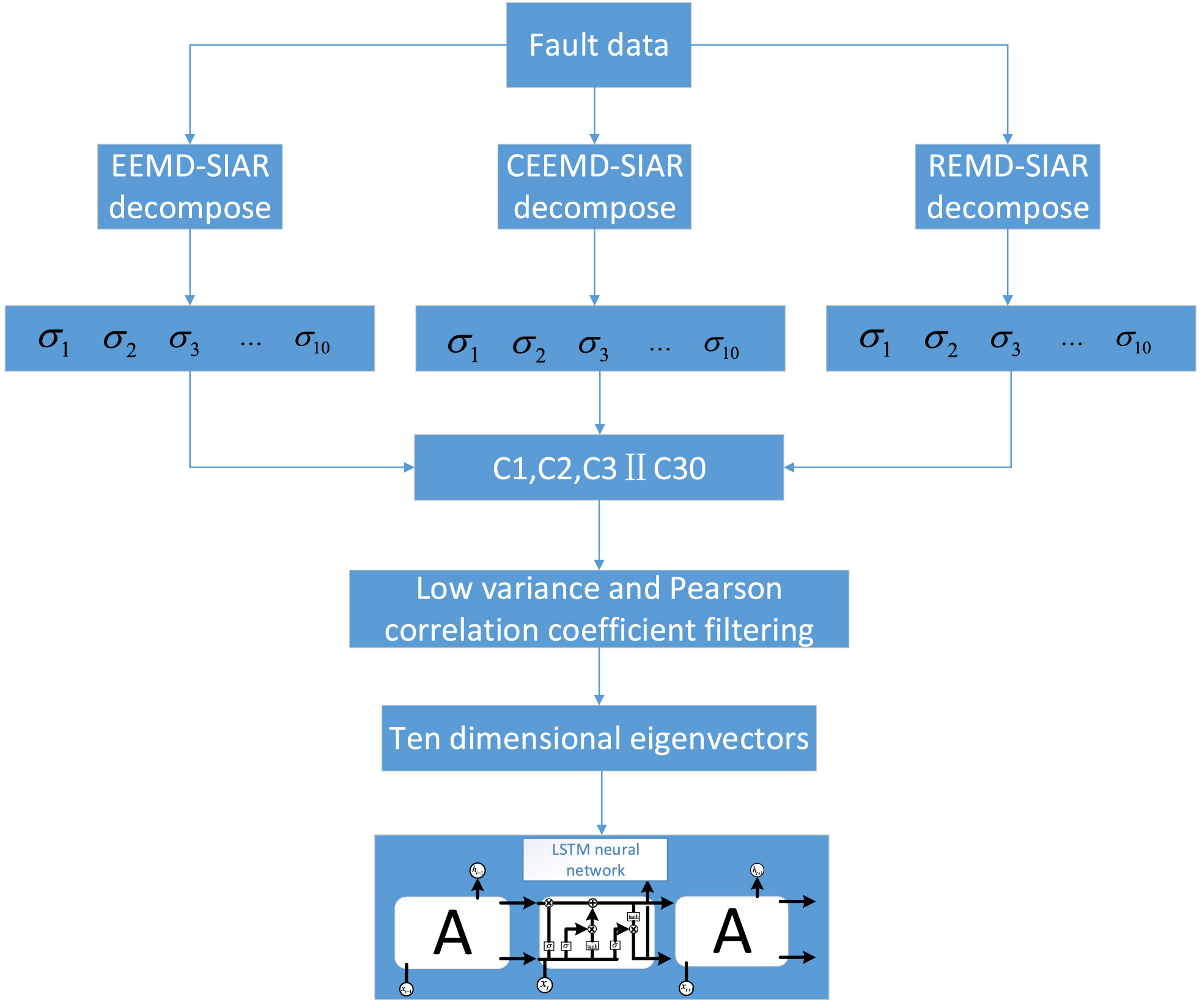
Flow chart of feature extraction based on information fusion and SIAR analysis.

4.2 BI-LSTM neural network

LSTM is an improvement on RNN. RNN is limited by its limited theoretical performance in dealing with the remote dependence problems due to gradient disappearance and gradient explosion. LSTM uses the gate structure and memory module to replace the hidden layer of RNN. The structure of LSTM unit is shown in Fig. 15 [24]. As shown in Fig. 15, LSTM stores and processes information mainly through three structures: input gate (i), forgetting gate (f) and output gate (o). X represents the input data, h represents the output of data, and C is the memory unit of storage location.

Fig. 15

LSTM structure diagram.

$C^{\sim (t)} = tanh (W_{xc} x^{t - 1} + W_{hc} h^{t - 1} + b_{c})$ (6)

LSTM was originally designed with only one-way data processing function, but the bi-directional LSTM was proposed after in-depth study. Bi-LSTM can lock the data in the model so that the current input and the data in the sequence before and after have a certain relationship, and the hidden layer stores the bi-directional sequence information, namely historical information and future information. Its structure is mainly composed of two LSTM models and two hidden layers, as shown in Fig. 16. Equation (7) is the update process of LSTM layer [25].

Fig. 16

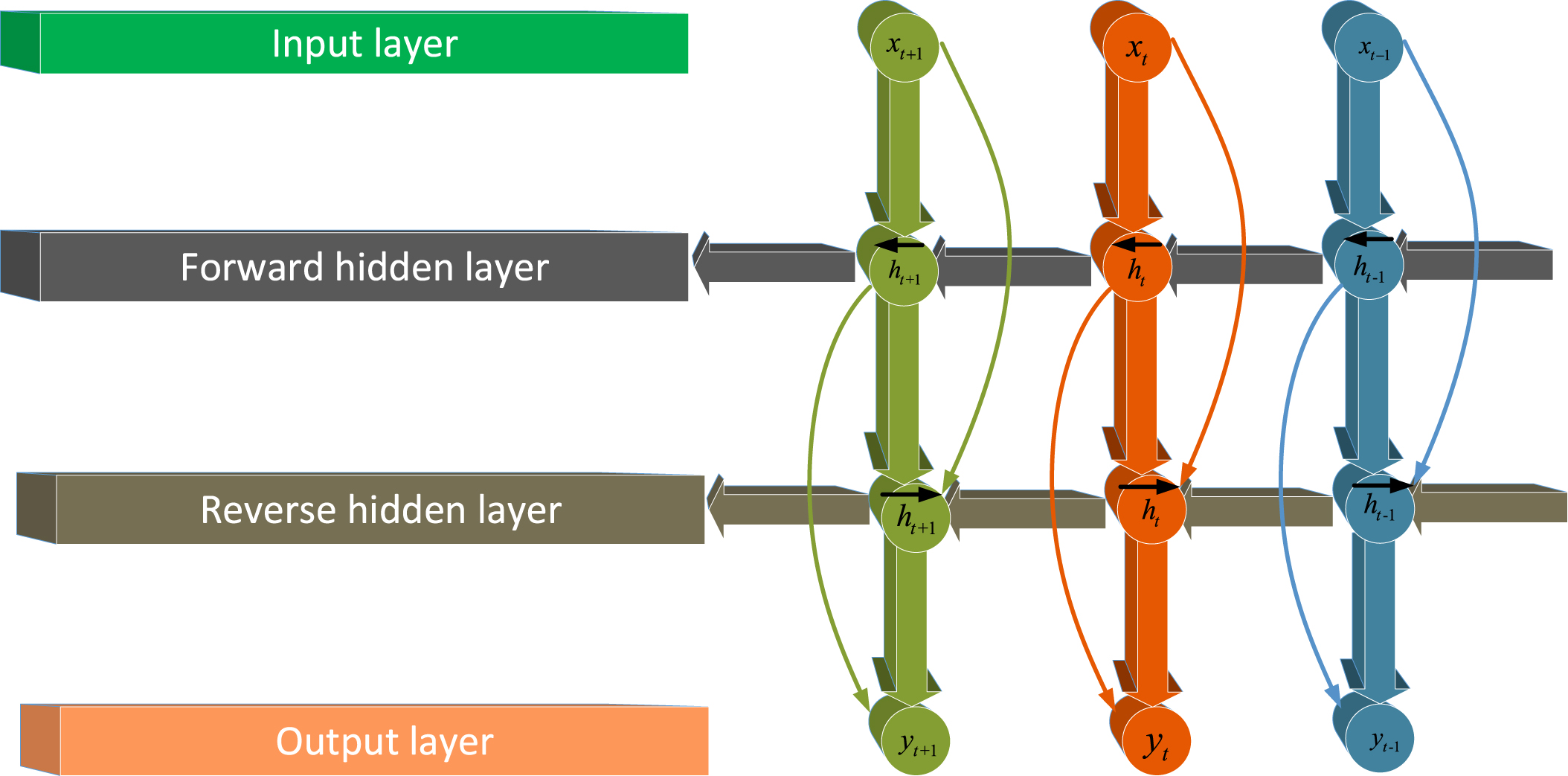
Structure diagram of bi-directional LSTM.

${\vec{h}}_{t} = H (W_{x {\vec{h}}_{t}} x_{t} + W_{{\vec{h}}_{t} {\vec{h}}_{t}} {\vec{h}}_{t - 1} + b_{\vec{h}})$ (7)

The updating process of LSTM layer from front to back can be expressed by Equation (8). $h_{t}^{\leftarrow} = H (W_{x h_{t}^{\leftarrow}} x_{t} + W_{h_{t}^{\leftarrow} h_{t}^{\leftarrow}} h_{t - 1}^{\leftarrow} + b_{\overset{\leftarrow}{h}})$ (8)

5 Fault diagnosis experiment simulation and result analysis

In this experiment, the rolling bearing fault signal data from Case Western Reserve University in the United States were used. In order to verify the effectiveness of the segmented AR spectral value-information fusion method described in this paper, the early bearing fault signals, namely damage diameter with 0.007 mm, were selected for effect verification. The experimental data and information are shown in Table 2. In the light of the collected experimental data of time sequence, the bi-directional LSTM neural network was selected as classifier. Initialize the network hidden layer as 50, a maximum 100 training cycle and fault category. A total of four data types respectively are the inner ring fault (1), outer ring fault (2) and rolling body (3) and normal data (4). A total of 400 groups of data with damage diameter of 0.007 mm were selected, 100 groups of data for each category, with sampling points of 1000 and sampling frequency of 48KHz. 400 groups of experimental data in Figs. 4 , 9 and 13 after processing are to get a set of data from 400 row 10 column matrix, as shown in Table 3 –5. Based on the flowchart shown in Fig. 14, the characteristics of the data set is obtained based on the further fusion process, and the fused data set shown in Table 6 is obtained according to the random disturb.

Table 2
Experimental data information

Bearing fault position Number of samples Single sample data points Damage to the diameter Category

Inner ring fault 100 1000 0.007 1

Outer ring fault 100 1000 0.007 2

Rolling fault 100 1000 0.007 3

Normal 100 1000 0 4

Bearing fault position	Number of samples	Single sample data points	Damage to the diameter	Category
Inner ring fault	100	1000	0.007	1
Outer ring fault	100	1000	0.007	2
Rolling fault	100	1000	0.007	3
Normal	100	1000	0	4

Table 3

EEMD-SIAR feature extraction results

Sample number	C1	C2	C3	C4	C5	. . .	C10	Category
1	–29.9304	–29.9778	–30.0221	–30.0633	–30.1017	. . .	–30.2526	1
2	–29.7641	–29.7994	–29.8318	–29.8614	–29.8884	. . .	–29.9886	1
3	–30.1636	–30.1803	–30.1939	–30.2042	–30.2116	. . .	–30.2094	1
4	–30.6859	–30.7282	–30.7677	–30.8042	–30.8381	. . .	–30.9717	1
5	–30.3571	–30.3692	–30.3777	–30.3827	–30.3845	. . .	–30.3488	1
. . .	. . .	. . .	. . .	. . .	. . .	. . .	. . .
100	–29.9657	–30.0084	–30.0484	–30.0856	–30.1201	. . .	–30.2577	1
101	–33.7015	–33.7563	–33.8064	–33.8517	–33.8925	. . .	–34.0290	2
102	–34.5233	–34.5646	–34.6021	–34.6358	–34.6660	. . .	–34.7666	2
103	–34.1706	–34.2422	–34.3095	–34.3726	–34.4315	. . .	–34.6675	2
104	–33.7562	–33.8163	–33.8722	–33.9240	–33.9717	. . .	–34.1520	2
105	–34.2661	–34.3209	–34.3715	–34.4182	–34.4610	. . .	–34.6196	2
. . .	. . .	. . .	. . .	. . .	. . .	. . .	. . .
200	–34.0805	–34.1665	–34.2493	–34.3291	–34.4060	. . .	–34.7509	2
201	–18.8113	–18.5863	–18.35123	–18.1094	–17.8657	. . .	–16.9061	3
202	–17.4059	–17.3117	–17.2215	–17.1397	–17.0709	. . .	–17.1113	3
203	–20.8550	–20.5434	–20.2043	–19.8379	–19.4451	. . .	–17.2743	3
204	–21.8798	–21.4695	–21.0154	–20.5138	–19.9610	. . .	–16.4315	3
205	–21.0513	–20.6586	–20.2249	–19.7483	–19.2274	. . .	–16.1723	3
. . .	. . .	. . .	. . .	. . .	. . .	. . .	. . .
300	–23.0122	–22.5636	–22.0602	–21.4949	–20.8594	. . .	–16.3183	3
301	–55.1270	–55.20961	–55.28812	–55.3626	–55.4333	. . .	–55.7311	4
302	–55.0949	–55.1786	–55.2582	–55.3339	–55.4058	. . .	–55.7093	4
303	–55.0424	–55.1214	–55.1965	–55.2678	–55.3353	. . .	–55.6191	4
304	–55.4932	–55.5783	–55.6591	–55.7358	–55.8084	. . .	–56.1145	4
305	–54.1047	–54.1968	–54.2851	–54.3697	–54.4505	. . .	–54.7992	4
. . .	. . .	. . .	. . .	. . .	. . .	. . .	. . .
400	–54.4434	–54.5257	–54.6042	–54.6790	–54.7501	. . .	–55.0508	4

Table 4

CEEMD-SIAR feature extraction results

Sample number	C1	C2	C3	C4	C5	. . .	C10	Category
1	–29.5368	–29.5882	–29.6375	–29.6848	–29.7302	. . .	–29.9323	1
2	–29.9508	–29.9841	–30.0149	–30.0432	–30.0692	. . .	–30.1682	1
3	–29.9619	–29.9794	–29.9946	–30.0075	–30.0185	. . .	–30.0491	1
4	–30.7600	–30.7990	–30.8351	–30.8684	–30.8990	. . .	–31.0160	1
5	–30.1752	–30.1903	–30.2026	–30.2120	–30.21893	. . .	–30.2194	1
. . .	. . .	. . .	. . .	. . .	. . .	. . .	. . .
100	–30.1038	–30.1398	–30.1729	–30.2031	–30.2307	. . .	–30.3323	1
101	–33.7158	–33.7563	–33.7921	–33.8233	–33.8499	. . .	–33.9173	2
102	–34.7064	–34.7359	–34.7614	–34.7830	–34.8009	. . .	–34.8387	2
103	–33.8980	–33.9653	–34.0288	–34.0887	–34.1451	. . .	–34.3771	2
104	–33.8194	–33.8648	–33.9060	–33.9431	–33.9762	. . .	–34.0846	2
105	–34.0349	–34.08930	–34.1403	–34.1882	–34.2329	. . .	–34.4129	2
. . .	. . .	. . .	. . .	. . .	. . .	. . .	. . .
200	–33.9439	–34.03984	–34.1333	–34.2246	–34.3136	. . .	–34.7289	2
201	–18.6911	–18.5374	–18.3807	–18.2245	–18.0729	. . .	–17.5906	3
202	–17.5661	–17.5179	–17.4746	–17.4393	–17.4156	. . .	–17.6066	3
203	–20.3357	–20.0494	–19.7445	–19.4230	–19.0880	. . .	–17.4787	3
204	–21.4384	–21.0429	–20.6089	–20.1340	–19.6166	. . .	–16.5201	3
205	–20.4917	–20.1340	–19.7443	–19.3229	–18.8715	. . .	–16.4835	3
. . .	. . .	. . .	. . .	. . .	. . .	. . .	. . .
300	–22.1029	–21.6432	–21.1326	–20.5657	–19.9372	. . .	–15.8640	3
301	–51.7250	–51.8080	–51.8871	–51.9623	–52.0338	. . .	–52.3344	4
302	–51.6777	–51.7516	–51.8217	–51.8882	–51.9510	. . .	–52.2107	4
303	–51.0624	–51.1458	–51.2251	–51.3004	–51.3717	. . .	–51.6684	4
304	–53.3311	–53.4046	–53.4744	–53.5406	–53.6031	. . .	–53.8621	4
305	–52.9972	–53.0658	–53.1308	–53.1924	–53.2506	. . .	–53.4901	4
. . .	. . .	. . .	. . .	. . .	. . .	. . .	. . .
400	–52.2119	–52.2665	–52.3176	–52.3655	–52.4099	. . .	–52.5819	4

Table 5

REMD-SIAR feature extraction results

Sample number	C1	C2	C3	C4	C5	. . .	C10	Category
1	–30.0557	–30.1037	–30.1485	–30.1903	–30.2290	. . .	–30.3812	1
2	–29.6532	–29.6951	–29.7345	–29.7716	–29.8065	. . .	–29.9521	1
3	–30.3063	–30.3287	–30.3477	–30.3633	–30.3758	. . .	–30.3947	1
4	–31.1369	–31.1715	–31.2023	–31.2294	–31.2528	. . .	–31.3205	1
5	–30.7296	–30.7468	–30.7597	–30.7684	–30.7730	. . .	–30.7389	1
. . .	. . .	. . .	. . .	. . .	. . .	. . .	. . .
100	–30.2593	–30.2950	–30.3272	–30.3561	–30.3817	. . .	–30.4652	1
101	–34.8727	–34.8991	–34.9191	–34.9328	–34.9400	. . .	–34.8817	2
102	–34.9453	–34.9670	–34.9839	–34.9961	–35.0037	. . .	–34.9772	2
103	–34.8798	–34.9199	–34.9545	–34.9836	–35.0072	. . .	–35.0477	2
104	–34.4831	–34.5183	–34.5480	–34.5722	–34.5910	. . .	–34.6068	2
105	–34.6719	–34.7088	–34.7409	–34.7682	–34.7907	. . .	–34.8363	2
. . .	. . .	. . .	. . .	. . .	. . .	. . .	. . .
200	–34.5313	–34.5809	–34.6262	–34.6674	–34.7047	. . .	–34.8379	2
201	–18.6564	–18.4559	–18.2486	–18.0382	–17.8296	. . .	–17.0846	3
202	–17.4782	–17.4291	–17.3848	–17.3484	–17.3236	. . .	–17.5124	3
203	–20.9391	–20.6388	–20.3118	–19.9582	–19.5789	. . .	–17.4676	3
204	–21.9290	–21.5276	–21.0830	–20.5915	–20.0494	. . .	–16.5658	3
205	–20.9848	–20.5911	–20.1566	–19.6794	–19.1586	. . .	–16.1348	3
. . .	. . .	. . .	. . .	. . .	. . .	. . .	. . .
300	–22.8891	–22.4407	–21.9383	–21.3751	–20.7432	. . .	–16.2819	3
301	–55.1073	–55.1768	–55.2426	–55.3048	–55.3636	. . .	–55.6067	4
302	–55.0898	–55.1725	–55.2513	–55.3261	–55.3970	. . .	–55.6967	4
303	–54.8944	–54.9692	–55.0403	–55.1079	–55.1718	. . .	–55.4399	4
304	–55.4385	–55.5163	–55.5901	–55.6601	–55.7264	. . .	–56.0041	4
305	–54.0840	–54.1744	–54.2611	–54.3442	–54.4236	. . .	–54.7666	4
. . .	. . .	. . .	. . .	. . .	. . .	. . .	. . .
400	–54.5910	–54.6529	–54.7115	–54.7667	–54.8186	. . .	–55.0295	4

Table 6

Feature extraction results based on SIAR and information fusion

Sample number	C1	C2	C3	C4	C5	. . .	C10	Category
1	–34.7071	–34.7471	–34.7837	–34.8170	–34.6152	. . .	–35.4141	2
2	–30.8659	–30.8753	–30.8821	–30.8866	–30.7683	. . .	–31.3454	1
3	–34.4763	–34.5365	–34.5939	–34.6487	–34.5121	. . .	–35.07409	2
4	–30.2435	–30.2675	–30.2891	–30.30833	–30.1518	. . .	–30.4964	1
5	–18.6908	–17.9739	–17.2129	–16.4315	–17.16634	. . .	–16.5658	3
. . .	. . .	. . .	. . .	. . .	. . .	. . .	. . .
100	–16.520	–16.5171	–16.5767	–16.7046	–16.4865	. . .	–16.3284	3
101	–17.6758	–17.2640	–16.8969	–16.6065	–17.0258	. . .	–16.6757	3
102	–55.4594	–55.5161	–55.5693	–55.6191	–51.6170	. . .	–55.4399	4
103	–17.5217	–16.9306	–16.3443	–15.8003	–16.3539	. . .	–15.8187	3
104	–54.8013	–54.8665	–54.9281	–54.9860	–52.3648	. . .	–54.9517	4
105	–55.8898	–55.9410	–55.9890	–56.0337	–52.7469	. . .	–55.9456	4
. . .	. . .	. . .	. . .	. . .	. . .	. . .	. . .
200	–19.5314	–18.6636	–17.7083	–16.6821	–17.4002	. . .	–16.6863	3
201	–30.8038	–30.8218	–30.8376	–30.8512	–30.5485	. . .	–31.0747	1
202	–54.6010	–54.6707	–54.7368	–54.7992	–53.44902	. . .	–54.7666	4
203	–55.5637	–55.6211	–55.6750	–55.7254	–50.96125	. . .	–55.5866	4
204	–34.8096	–34.8495	–34.8857	–34.91837	–34.5476	. . .	–35.1342	2
205	–29.9415	–29.9663	–29.9894	–30.01090	–29.9449	. . .	–30.2903	1
. . .	. . .	. . .	. . .	. . .	. . .	. . .	. . .
300	–34.5357	–34.5714	–34.6035	–34.6321	–33.7144	. . .	–34.9883	2
301	–34.5183	–34.5516	–34.5808	–34.6061	–34.6448	. . .	–35.0461	2
302	–30.7857	–30.8110	–30.8341	–30.8551	–30.7838	. . .	–30.9722	1
303	–55.1027	–55.1617	–55.2174	–55.2699	–52.6756	. . .	–55.1974	4
304	–30.1040	–30.1290	–30.1517	–30.17248	–29.8033	. . .	–30.6033	1
305	–55.3674	–55.4231	–55.4756	–55.5243	–49.1020	. . .	–55.4961	4
. . .	. . .	. . .	. . .	. . .	. . .	. . .	. . .
400	–18.6680	–17.7849	–16.8288	–15.8341	–16.9384	. . .	–16.1712	3

Figures 17 19 are the simulation test results based on SI-AR with EEMD, CEEMD and REMD, where the red cross represents the actual label of the test samples, and the blue circle represents the predicted values. The simulation results show that there is little difference between the three algorithms. The accuracy of EEMD-SIAR, CEEMD-SIAR and REMD-SiAR for fault diagnosis is 96%, 95% and 92% respectively. Figure 20 shows the simulation test results of information fusion on the eigenvalues under three processed algorithms. The results show that the diagnostic accuracy was 100%, thus further diagnostic accuracy of the information integration of the accurate rate is higher than that of single algorithm after processing. On the other hand, the other fault diagnosis models are compared with the proposed fault diagnosis model.

Fig. 17

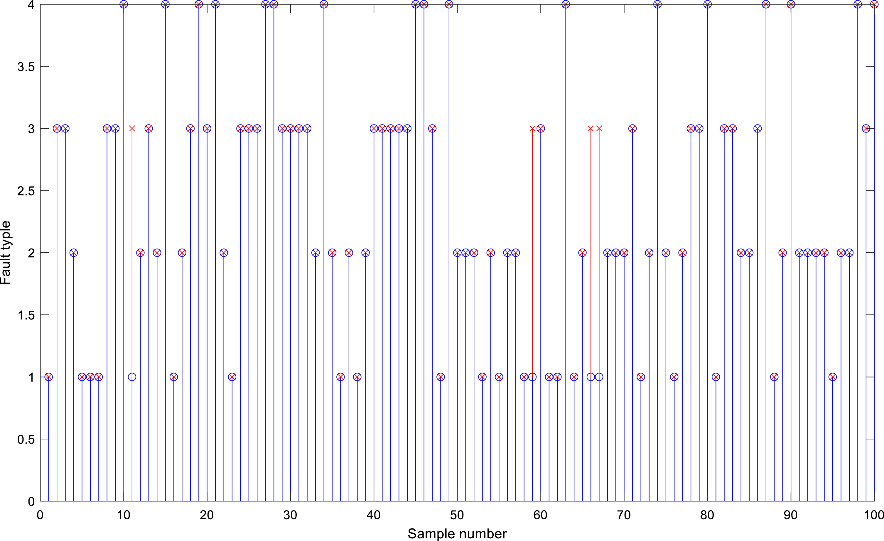
Simulation test results of EEMD-SIAR (96%).

Fig. 18

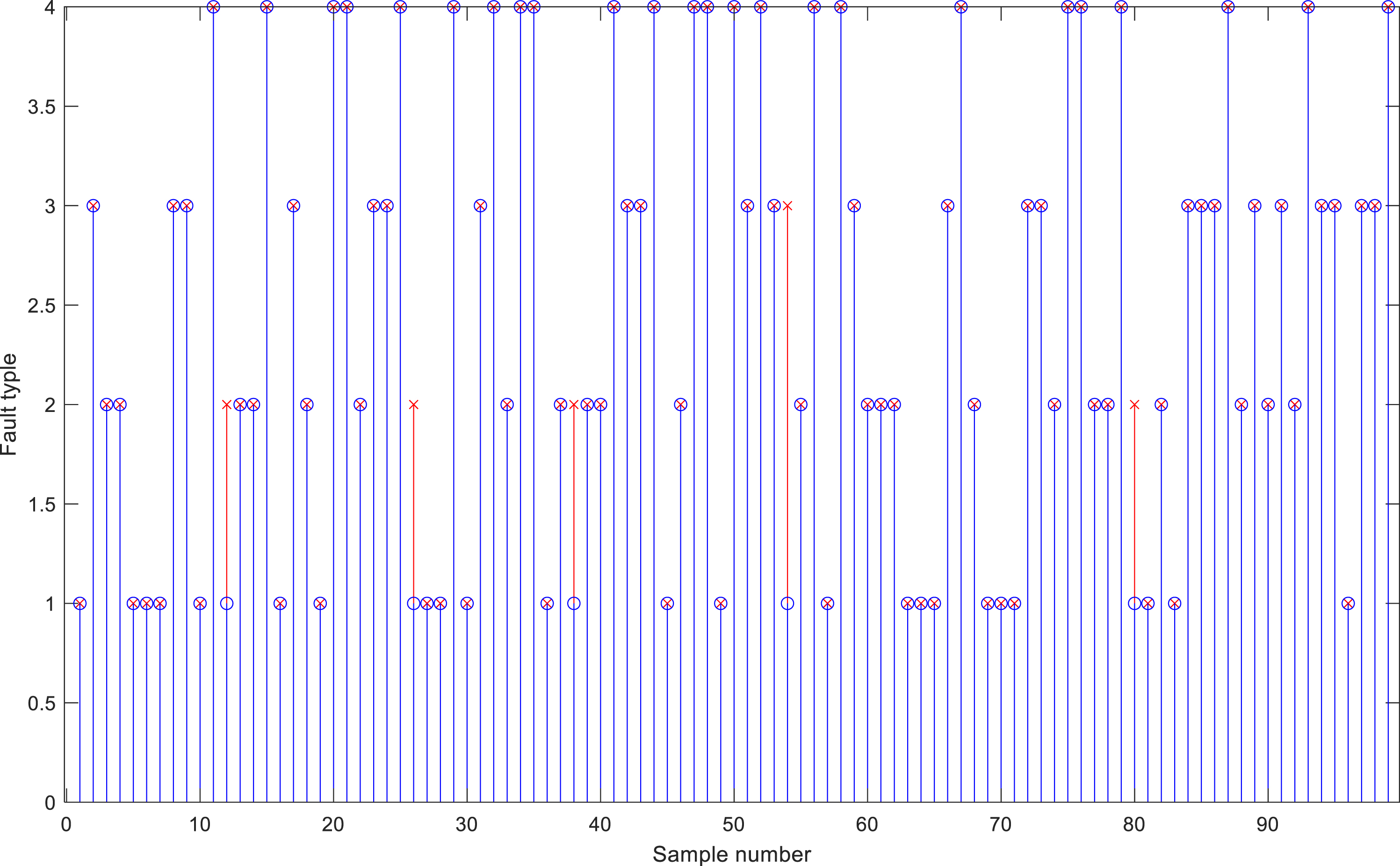
Simulation test results of CEEMD-SIAR (95%).

Fig. 19

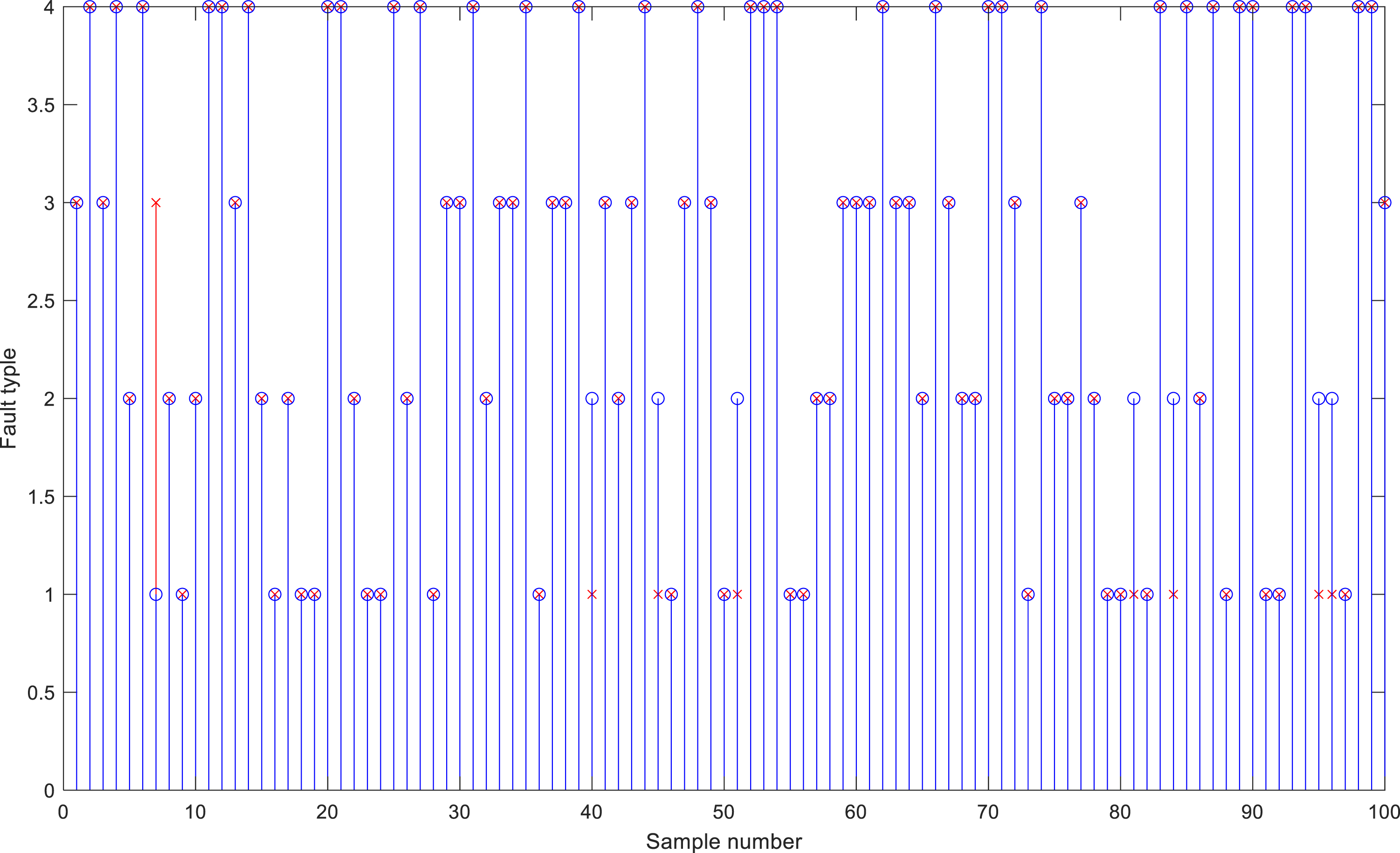
Simulation test results of REMD-SIAR (92%).

Fig. 20

Simulation test results of SIAR-information fusion (100%).

It can be seen from Table 7, various fault diagnosis models proposed by scholars have achieved good results. For example, Wang et al. proposed a new multi-sensor information fusion method to realize fault classification. In this method, the time-domain vibration signals from multiple sensors at different locations were constructed into a rectangular two-dimensional matrix, and then the improved two-dimensional CNN was used to realize signal classification. The results were verified on the Case Western Reserve University data set, the IMS bearing database and the designed bearing failure test bed data set, and the prediction accuracy was 99.92%, 99.68% and 99.25%, respectively. Compared with traditional fault classification methods such as 1D and 2D CNN, this model can use less data and computational complexity to achieve higher fault prediction accuracy. Qi et al. proposed a new fault diagnosis model based on fault rate and fault symptom, In this method, the information of failure rate, failure mechanism and fault symptom was considered comprehensively, and the information of these fault characteristics was fused, with a correct rate of 87.5%. Li et al. proposed a deep stacking least squares support vector machine model for fault diagnosis, with a correct rate of 99.90%. Konar and Chattopadhyay proposed a continuous wavelet transform model, whose accuracy was only 90%. The fault diagnosis model proposed in this paper was based on the traditional signal analysis algorithms and its varients, which analyzed the fault signal and fuses the extracted features. It can be seen from the results that the prediction accuracy rate of the proposed diagnosis model is up to 100%, which is superior to the fault diagnosis ability of most other models and can be effectively used for bearing fault diagnosis.

Table 7

Comparison results of rolling bearing fault diagnosis models

Author	Fault diagnosis model	Data set	Fault type	Diagnostic accuracy
Li [26]	Fuzzy Lattice Classifier (FLC)	Case Western Reserve University Bearing Failure Database (CWRU)	Normal state (NS), Inner ring fault (IRF), Outer ring fault (ORF) and Rolling fault (BF)	92%
Konar and Chattopadhyay [27]	Continuous Wavelet Transform (CWT)	Experimental data collected by the authors	Normal state (NS) Fault state (FS)	90 %
Pan [28]	Symplectic Geometry Matrix Machine (SGMM)	CWRU	NS, ORF, IRF and BF	99.83%
Li [29]	Deep Stacking Least Squares Support Vector Machine (DSLS-SVM)	CWRU	NS, ORF, IRF and BF	99.90%
Wang [30]	A new multi-sensor information fusion method	CWRU IMS Self-made test rig respectively	NS, ORF, IRF and BF	99.92% 99.68% 99.25%
Qi [13]	New fault diagnosis model based on fault rate and fault symptom	CWRU	NS and FS	87.5%
This paper	EEMD-SIAR	CWRU	NS, ORF, IRF and BF	96%
	CEEMD-SIAR	CWRU	NS, ORF, IRF and BF	95%
	REMD-SIAR	CWRU	NS, ORF, IRF and BF	92%
	Information fusion–SIAR	CWRU	NS, ORF, IRF and BF	100%

6 Conclusions

In order to solve the problem that there are invalid and redundant components in the decomposed components of the fault diagnosis algorithm, and it is easy to cause the loss of feature information when a single algorithm decomposes the signal to extract fault features. So this paper fragments the AR spectrum value as the eigenvalue of the fault data, and adopts EEMD, CEEMD and REMD algorithms to decompose the signal. The income components will be carried out the AR spectral analysis and the effective AR spectrum values are intercepted as the characteristic value of data. Then the characteristics of three kinds of algorithms about value information fusion avoid lost characteristics in order to achieve the purpose of more efficient screening effective characteristics. Finally it is verified by simulation results of fault data in this paper and the proposed method can be effectively used in the fault diagnosis of rolling bearing.

Although the current fault diagnosis method based on empirical mode decomposition and its related varients had unique advantages in the processing of non-stationary nonlinear signals, the algorithm still has the following problems to be solved. (1) Boundary effect. The boundary effect which is easy to appear in EMD decomposition has certain influence on signal analysis. Moreover, in the fitting process of upper and lower envelope during EMD decomposition, the fitting method is still cubic spline interpolation, which will cause serious boundary effect to pollute the original fault signals in practical engineering applications. As a result, the original fault signal loses some authenticity, which affects the diagnosis result and needs to be further improved to enhance its performance. (2) For the EEMD algorithm, although the addition of white noise and the elimination of invalid extreme points can inhibit the generation of mode aliasing phenomenon to a certain extent, it still cannot completely eliminate this phenomenon, and the process of adding white noise will produce some redundant components without practical physical significance, and there is no very effective method to effectively screen these redundant components.

Footnotes

Acknowledgments

This work was supported by the Basic Scientific Research Project of Institution of Higher Learning of Liaoning Province (Grant No. LJKZ0293 and LJKZ0307), and the Postgraduate Education Reform Project of Liaoning Province (Grant No. LNYJG2022137).

Conflict of interest

The authors declare that there is no conflict of interests regarding the publication of this article.

Author contributions

Cheng Zhong participated in the algorithm simulation and draft writing. Jie-sheng Wang participated in the concept, design, interpretation and critical revision of this paper. Yu Liu participated in the data collection and analysis of the paper.

References

Feng

, Zhao

, Gu

, et al., Efficient implementation of envelope analysis on resources limited wireless sensor nodes for accurate bearing fault diagnosis[J], Measurement 110 (2017), 307–318.

Xue

and Zhou

, Ahybrid fault diagnosis approach based on mixed-domain state features for rotating machinery[J], Isa Transactions, 2016.

Parey

and Pachori

R.B.

, Variable cosine windowing of intrinsic mode functions: Application to gear fault diagnosis[J], Measurement 45(3) (2012), 415–426.

Wang

Y.S.

, Ma

Q.H.

, Zhu

, et al., An intelligent approach for engine fault diagnosis based on Hilbert–Huang transform and support vector machine[J], Applied Acoustics 75(1) (2014), 1–9.

Guo

and Deng

, An improved EMD method based on the multi-objective optimization and its application to fault feature extraction of rolling bearing[J], Applied Acoustics 127 (2017), 46–62.

, Wang

and Makis

, Fault severity recognition of aviation piston pump based on feature extraction of EEMD paving and optimized support vector regression model[J], Aerospace Science & Technology 67 (2017), 105–117.

Deng

, Zhao

, Yang

, et al., A fault feature extraction method for motor bearing and transmission analysis[J], Symmetry 9(5) (2017), 60.

Yeh

J.R.

, Shieh

J.S.

and Huang

N.E.

, Complementary ensemble empirical mode decomposition: a novel noise enhanced data analysis method[J], Advances in Adaptive Data Analysis 02(02) (2010), 135–156.

Lei

, Liu

and Ouazri

, A Fault diagnosis method of rolling element bearings based on CEEMDAN, Archive Proceedings of the Institution of Mechanical Engineers Part C Journal of Mechanical Engineering Science 203–210 (2015), 1989–1996.

10.

and Liu

S.Q.

, Gearbox fault diagnosis based on EMD-AR spectrum analysis and SVM, Machinery Design & Manufacture 11 (2021), 56–64.

11.

Cai

J.H.

, Liu

and Yang

J.H.

, Analysis of 3C 273 photovarying period based on EMD-AR spectrum, Journal of Astronomy 63(1) (2022).

12.

, Cheng

, Ding

, et al., Method for extracting fault feature information of multi-axis rotor system based on VMD-AR spectrum, Journal of Jiangsu Uivesity 41(5) (2020), 563–568.

13.

J.Y.

and Wang

L.Y.

, Fault diagnosis method of equipment based on multi-information fusion, International Journal of Plant Engineering and Management 25(2) (2020), 78–96.

14.

Tang

, Hu

T.H.

, Chen

, et al., A deep convolutional neural network approach with information fusion for bearing fault diagnosis under different working conditions, Proceedings of the Institution of Mechanical Engineers, Part C: Journal of Mechanical Engineering Science, 2020, 095440622090218.

15.

Zvokelj

, Zupan

and Prebil

, EEMD-based multiscale ICA method for slewing bearing fault detection and diagnosis[J], Journal of Sound and Vibration 370 (2016), 394–423.

16.

, Lin

, Zhang

, et al., Faults diagnostics of railway axle bearings based on IMF’s confidence index algorithm for ensemble EMD[J], Sensors 15(5) (2015), 10991–11011.

17.

Yoon

and He

, Planetary gearbox fault diagnostic method using acoustic emission sensors[J], Science Measurement and Technology Iet 9(8) (2015), 936–944.

18.

Sheng

, Monitoring of wind turbine gearbox condition through oil and wear debris analysis: a full-scale testing perspective[J], Tribology Transactions 59(1) (2016), 149–162.

19.

, Yan

and Silva

C.W.D.

, Dominant feature selection for the fault diagnosis of rotary machines using modified genetic algorithm and empirical mode decomposition[J], Journal of Sound & Vibration 344 (2015), 464–483.

20.

, Wang

, Tang

, et al., An improved method based on ceemd for fault diagnosis of rolling bearing[J], Advances in Mechanical Engineering 7 (2014), 175–184.

21.

Peng

, Bo

and Xie

X.L.

, Rolling bearing fault diagnosis method based on eemd, metric factor and fast kurtosis graph [J], Vibration and Shock 31(20) (2012), 143–146.

22.

Xing

H.Y.

and Zhu

Q.Q.

, Sea clutter denoising based on integrated empirical mode decomposition [J], Acta Electronica Sinica 44(1) (2016), 1–7.

23.

Singh

, Howard

C.Q.

and Hansen

C.H.

, An extensive review of vibration modelling of rolling element bearings with localised and extended defects[J], Journal of Sound & Vibration 357 (2015), 300–330.

24.

Liang

, Wang

, Wu

, et al., Elimination of end effects in LMD based on LSTM network and applications for rolling bearing fault feature extraction, Math Probl Eng (2020), 1–16.

25.

Mei

, Wu

and Li

, Fault diagnosis and remaining useful life estimation of aero engine using LSTM neural network, IEEE/CSAA International Conferenceon Aircraft Utility Systems, 2016.

26.

, Liu

P.Y.

, Hu

, et al., Fuzzy lattice classifier and its application to bearing fault diagnosis, Applied Soft Computing 12(6) (2012), 1708–1719.

27.

Konar

and Chattopadhyay

, Bearing fault detection of induction motor using wavelet and support vector machines (SVMs), Applied Soft Computing 11(6) (2011), 4203–4211.

28.

Pan

, Yang

, Zheng

, et al., A fault diagnosis approach for roller bearing based on symplectic geometry matrix machine, Mechanism and Machine Theory 140 (2019), 31–43.

29.

, Yang

, Pan

, et al., A novel deep stacking least squares support vector machine for rolling bearing fault diagnosis, Computers in Industry 110 (2019), 36–47.

30.

Wang

J.X.

, Wang

D.Z.

, Wang

S.H.

, et al., Fault diagnosis of bearings based on multi-sensor information fusion and 2d convolutional neuralnetwork, IEEE Access (2021), 23717–23725.

Bi-LSTM fault diagnosis method for rolling bearings based on segmented interception AR spectrum analysis and information fusion

Abstract

Keywords

1 Introduction

2 Basic principle of AR spectrum estimation

3.1 Rolling bearing fault diagnosis signal analysis based on EEMD-AR

3.1.1 Basic principles of EEMD algorithm

3.2.1 Basic principles of CEEMD algorithm

4.1 Rolling bearing fault diagnosis method based on SIAR and information fusion

Table 2 Experimental data information Bearing fault position Number of samples Single sample data points Damage to the diameter Category Inner ring fault 100 1000 0.007 1 Outer ring fault 100 1000 0.007 2 Rolling fault 100 1000 0.007 3 Normal 100 1000 0 4

Footnotes

Acknowledgments

Conflict of interest

Author contributions

References

Table 2
Experimental data information

Bearing fault position Number of samples Single sample data points Damage to the diameter Category

Inner ring fault 100 1000 0.007 1

Outer ring fault 100 1000 0.007 2

Rolling fault 100 1000 0.007 3

Normal 100 1000 0 4