Group-individual multi-mode cooperative teaching-learning-based optimization algorithm and an industrial engineering application

Abstract

This paper modifies the original Teaching-Learning-based Optimization (TLBO) algorithm to present a novel Group-Individual Multi-Mode Cooperative Teaching-Learning-based Optimization (CTLBO) algorithm. This algorithm introduces a new preparation phase before the teaching and learning phases and applies multiple teacher-learner cooperation strategies in teaching and learning processes. In the preparation phase, teacher-learner interaction and teacher self-learning mechanism are applied. In the teaching phase, class-teaching and performance-based group-teaching operators are applied. In the learning phase, neighbor learning, student self-learning and team-learning strategies are mixed together to form three operators. Experiments indicate that CTLBO has significant improvement in accuracy and convergence ability compared with original TLBO in solving large scale problems and outperforms other compared variants of TLBO in literature and other 9 meta-heuristic algorithms. A large-scale industrial engineering problem—warehouse materials inventory optimization problem is taken as application case, comparison results show that CTLBO can effectively solve the large-scale real problem with 1000 decision variables, while the accuracies of TLBO and other meta-heuristic algorithm are far lower than CLTBO, revealing that CTLBO can far outperform other algorithms. CTLBO is an excellent algorithm for solving large scale complex optimization issues.

Keywords

Teaching-learning-based optimization group-individual multi-mode cooperation performance-based group teaching teacher self-learning team learning

1 Introduction

Intelligent optimization algorithms are some special techniques for overcoming the shortcomings of traditional OR (operations research) methods, and usually are applied to solve large, complex engineering and science problems. It is reported that more than 200 types of intelligent algorithms have been developed [1] in the last three decades.

Teaching-Leaning-based Optimization (TLBO) algorithm is one kind of population-based human-inspired optimization algorithms, it imitates the human knowledge spreading by teaching and learning behaviors [2]. Since its emergence, TLBO has been attracting more and more attentions. Compared with other algorithms, TLBO seems to be a rising star amongst a number of metaheuristics with its excellent performance [3]. Due to its some advantages, such as simple concept, rapid convergence, TLBO has been widely applied in solving single and multi-objective optimization issues in the fields of operations research, manufacturing system, mechanical and electrical engineering, civil engineering, electronics and control engineering, pattern recognition and image processing [4]. However, TLBO also has some shortcomings and limitations. For example, the algorithm also exists premature phenomena when solving complex optimizations problems. it still possible to be trapped in the local convergence phenomena [19]. Meanwhile, TLBO in fact does not really consider the multiple learning mechanisms in real-world, for example self-learning, individual difference in learning ability, etc. [13]. Therefore, in order to overcome these disadvantages of TLBO, some authors also have improved this algorithm by improving its teaching and learning mechanisms or mixing it with other algorithms to form hybrid TLBO algorithms. In most improved versions of TLBO, the main efforts have been made to improve the intrinsic search mechanism. These efforts mainly lie in two aspects: improving the teaching mechanism and improving the learning mechanism.

In the original TLBO, leaners update knowledge based on the teacher’s and the mean knowledge of the class. Zou et al. [5] improved TLBO by revising the teaching phase operator of the individual position update using the principle of PSO. Similarly, Shukla et al. [6] improved TLBO in the teaching phase, each learner’s knowledge update comes from the teacher and his own old knowledge. Tong et al. [7] improved TLBO as SLTLBO algorithm, in the teaching phase, learners improve their knowledge by learning from the difference between the teacher and the worst learner, Zou et al. [8] also improved the TLBO by introducing differential evolution (DE) operator into the teaching phase to increase the diversity of the new population. Tsai [9] improved TLBO algorithm as CTLBO, in the teaching phase of this algorithm, eight teaching strategies are constructed, in which, learner’s knowledge update is related to the difference between the teacher and the mean, or the difference between selected two learners. Wu et al. [10] proposed an improved TLBO algorithm (DI-TLBO), in the teaching phase, depending on a random number, a leaner gains knowledge from the teacher or from a randomly selected learner. Since original TLBO algorithm has only one teacher, so some authors introduced multiple teachers to enhance the algorithm search ability. Rao et al. [11], Vitayasak and Pongcharoen [12] adopted a multi-teacher concept to modify the teaching phase in TLBO algorithm. Ma et al. [13], Zhang and Jin [14] introduced group teaching strategy in TLBO teaching phase.

In the improvement of learning phase, there are also some literatures. Chen et al. [15] improved the learning phase by two strategies, the first strategy is to introduce a probability to decide whether a student learns from others or learns from the teacher and neighbors, and the second strategy is to introduce self-learning. Zou et al. [16] improved the TLBO as a new two-level hierarchical multi-swarm cooperative TLBO. Ji et al. [17] improved TLBO as I-TLBO, using historical population experience in self-feedback phase to improve learners’ results. Shao et al. [18] also improved the learning phase by changing the learning mechanism from neighborhood learning to mixed mechanism combing neighborhood learning with learning from the teacher. Zou et al. [8] improved the learning phase of TLBO, in which, learner’ knowledge update comes from learning from the teacher, neighbors and self-learning. Shukla et al. [6] also improved TLBO in the learning phase, differing from original TLBO only has learning from one neighbor, the improved version randomly selects three neighbors, learner’s knowledge update comes from other two neighbors. Similarly, Tsai [9] improved TLBO in learning phase by introducing four search strategies, in which, a learner updates knowledge based on the mutation with his(her) neighborhood or the mutation of other two randomly selected learners. Wu et al. [10] also improved TLBO in the learning phase; depending on a random number, a leaner gains knowledge from one randomly selected learner or randomly selected two learners. Xu et al. [19] proposed an improved TLBO algorithm as DOLTLBO, which employs a dynamic opposite learning strategy to overcome the algorithm drawback—premature convergence phenomenon.

He et al. [20] improved TLBO as chaotic teaching-learning based optimization with Levy flight (CTLBO). Dong et al. [21] also improved TLBO by introducing a two phases kriging-assisted optimization framework to alternately conduct local and global search. Similarly, Dong et al. [22] proposed another surrogate-assisted teaching and learning based optimization algorithm. Mittal et al. [23] improved TLBO by introducing a learning enthusiasm factor to enhance the exploration and exploitation ability, meanwhile, opposition-based learning, local neighborhood search techniques are also applied in the algorithm. Cheng and Prayogo [24] proposed an improved TLBO algorithm—fuzzy adaptive teaching learning optimization (FATLBO). Vitayasak and Pongcharoen [12] proposed a modified TLBO in which single teacher and multiple teachers are employed. Some authors introduced self-learning mechanism learning phase, for example, Rao and Patel [25], Yang et al. [26], Chen et al. [15], Ge et al. [27], Zou et al. [16], Chen et al.[28].

Although many authors have taken different efforts to improve TLBO to enhance its optimization ability, shortcomings also exist. Firstly, all improved algorithms continue to adopt the basic two-phase mechanism—teaching and learning, all improvement are conducted to improve these two phases. Secondly, most of those improved algorithms are only applied in small and small-medium sized cases, seldom applied to large size real problems. In this paper, we develop a new improved version of TLBO–multi-mode group-individual cooperative teaching-learning-based optimization (CTLBO), which applies multiple models of cooperation strategies in teaching and learning processes. CTLBO has several innovative contributions. Firstly, this algorithm introduces a new phase–preparation phase, while original TLBO and other variants of TLBO have only two phases-teaching and learning phases. In the preparation phase, a cooperation strategy between the teacher and students is introduced, then, a teacher self-learning strategy is first put forward in this paper, while all other variants of TLBO only employ self-learning mechanism in the learning phase. Secondly, in the teaching phase, in addition to the application of cooperation strategy in the class-teaching operator, this paper proposes a new performance-based multi-group teaching strategy. Thirdly, in the learning phase, a new cooperation mechanism mixed with neighbor learning, team-learning and self-learning is proposed. Multiple experiments show that this new algorithm reveals a significant performance improvement compared with original TLBO and other improved versions of TLBO, also, it has best performance compared with other 9 meta-heuristic algorithms. At last, in order to validate the effectiveness and feasibility of the CTLBO algorithm in solving large scale complex problems, a real case of hub warehouse materials inventory optimization issue of one automobile assembly factory is applied. The result shows that significant advantage of CTLBO compared with other meta-heuristic algorithms.

The remainder of this paper is organized as follows: the next section introduces the basic principle and algorithm description of TLBO, Section 3 develops the CTLBO algorithm, Section 4 conducts the experiment of numerical examples. Section 5 is the applications of algorithms in real world problems. Section 6 is the conclusions of the paper.

2 The Original TLBO algorithm

TLBO algorithm imitates the teaching and learning process in a class, the best solution is taken as the teacher, and other solutions are considered as learners(students). Simply, TLBO is divided into two phases, the first phase is called teaching phase, the second phase is called learning phase.

Suppose the optimization problem is min F = f (X), a population of learners composed of the teacher and students in a class represent a group optimization agents, each agent searches one optimization result, F_i . The number of the optimization agent is i = 1, . . . , NP, the decision dimension (number of variables) is j = 1, . . . , D (equal to the number of “subjects” of teaching in the class), the iteration number of the algorithm is t = 1, . . . , T_max. The position of i^th learner (includes the teacher and students) is presented as vector X_i = [x_i, 1, x_i, 2, ⋯ , x_i, D] _∘ then total leaners’ positions construct a matrix as: $X = [X_{1}, X_{2}, \dots, X_{N}] = [\begin{matrix} x_{1, 1} & \dots & x_{1, D} \\ ⋮ & ⋱ & ⋮ \\ x_{N, 1} & \dots & x_{N, D} \end{matrix}]$ (1) The lower and upper limits of the decision variables are L_b and U_b, i.e., x_i,j ∈ [L_b, U_b]. At beginning, a randomly generated initial solution is first set as: $x_{i, j} = L_{b} + rand (0, 1) * (U_{b} - L_{b}) .$ (2)

2.1 Teaching phase

The first search optimization phase of TLBO is teaching phase. In this phase, learners update their knowledge from the teacher and the mean state of the class is written as $X_{i}^{new} = X_{i} + \bar{R} \otimes (X_{teacher} - T_{f} \cdot X_{mean})$ (3) where $X_{i}^{new}$ is the updated position of i^th learner from current position X_i, $\bar{R}$ is a random vector with dimension number equals the decision variables (D); $X_{Teacher} = \underset{i}{argmin} (f (x_{1}), f (x_{2}, \dots, f (x_{NP}))$ is the teacher (the best solution); $X_{mean} = \frac{1}{NP} \sum_{i = 1}^{NP} X_{i}$ which is the mean level of the class. T_f is teaching factor, T_f = round [1 + rand (0, 1)] which equals 1 or 2 and is randomly generated during iteration.

2.2 Learning phase

After finishing the teaching phase, TLBO enters the second phase—learning phase. In this phase, learners update their knowledge by interacting with other learners, this process is finished by neighbor learning mechanism. A learner randomly selects a neighbor to learn and update his(her) knowledge (solution position). This procedure can be expressed as: $X_{i}^{new} = {\begin{matrix} X_{i} + \vec{R} \otimes (X_{i} - X_{j}), if F (X_{i}) < F (X_{j}) \\ X_{i} + \vec{R} \otimes (X_{j} - X_{i}), if F (X_{j}) < F (X_{i}) \end{matrix}$ (4)

3 CTLBO algorithm

We improve the original TBLO by introducing multi-mode group-individual cooperation mechanism, enhancing the convergence and global search ability of the algorithm. This new algorithm is composed of three phases—preparation phase, teaching phase and learning phase.

3.1 Preparation phase

In this phase, we design two operators, the first one is called TLI (teacher-learner interaction) operator which initiates the cooperation between the teacher and students; the second one is called teacher self-learning (TSL) operator which reflects the teacher learns knowledge from her history experience.

(1) Teacher-learner interaction (TLI operator)

A TLI operator is a modified particle swarm algorithm module which has two equations, velocity and position equations. The velocity update equation is described as the following equation (5). $\begin{matrix} V_{i} = w_{10} * V_{i} + (1 - w_{10}) * (c_{10} * r 1 * (abs (X_{mean} \\ - Y_{i})) + c_{20} * r 2 * (abs (X_{Teacher} - Y_{i}))), \end{matrix}$ (5) where w₁₀ is an inertia weigh factor added to the velocity, its value is dynamic during iteration, i.e., $w_{10} = w_{10} * (1 - \frac{t}{T_{max}})$ . c₁₀ and c₂₀ are personal learning factor and social learning factor, respectively, r1 and r2 are two random numbers in the interval [0, 1] respectively, i.e., r1 = rand(0, 1), r2 = rand(0, 1). Y_i is the position of individual i.

The second equation is called position update which is addition of the original position and the velocity, the position update is described as $Y_{i} = {\begin{matrix} (Y_{i} + V_{i}) * OD, if rand > 0.5 \\ (Y_{i} - V_{i}) * OD, else, \end{matrix}$ (6) where $OD = (1 + q * \sin (360 * t / T_{\max}) * (1 + q * \cos (360 * \frac{i}{NP})$ , and is called oscillation factor, in which $q = q_{0} * (1 - \frac{t}{T_{\max}})$ . The oscillation factor becomes smaller and smaller with the iteration number increases. Thus, when the algorithm converges to the optimal area, the oscillation factor becomes zero.

(2) Teacher self-learning (TSL operator)

As best as we known, the original TLBO and all other variants of TLBO have not applied self-learning mechanism in teaching phase. In this paper, we employ a teacher self-learning mechanism to enhance the “knowledge” of the teacher. Our teacher self-learning mechanism includes three selective channels. The first channel is call incentive weighted summation, the second channel is called incentive weighted summation with Levy flight exploitation, and the third channel is called random incentive difference. During iteration, three selection switch doors are determined by a random number.

(i) Channel I: incentive weighted summation

In this channel, the self-learned knowledge of the teacher is updated from the historical knowledge of the whole class including students and himself. We introduce an incentive factor for the knowledge update; thus, the self-learned knowledge of the teacher is calculated as follows. $Δ 1 L_{v} {GG (t) + TS L_{1} * GG (t - 1)}$ (7) where Δ1 is the obtained knowledge by teacher self-learning in channel I, GG (t) and GG (t - 1) are the global best knowledge of the whole class (including teacher and students) in the t^th and (t - 1) ^th teaching-learning processes, i.e. the global best solutions during the t^th and (t - 1) ^th iterations. $TS L_{1} = \frac{2}{1 + \exp (1 - \frac{t}{T_{\max}})}$ is called the incentive factor of GG(t-1). The incentive factor of GG(t) is set as 1. In order to reflect the self-learning ability of the teacher, we set a learning rate parameter, $L_{v} = 2 * (1 - \frac{t}{T_{\max}}) L_{0}$ , where L₀ = 2 * rand (0, 1) - 1 . This parameter will decrease to zero during the process of iteration.

Finally, the self-learned knowledge update of the teacher by the channel I is set as follows. $Z^{new} = Z^{current} + Δ 1$ (8) where Z^current is the current knowledge of the teacher, it is dynamic value during iteration, in this paper, Z^current = X_Teacher. $Z^{new} = X_{Teacher}^{new}$ , is updated knowledge of the teacher.

Substitute Δ1 of equation (7) into (8), the final knowledge update equation is as follows: $\begin{matrix} Z^{new} = Z^{current} + L_{v} * {GG (t) + TS L_{1} \\ * GG (t - 1)} . \end{matrix}$ (9)

(ii) Channel II: incentive weighted summation with Levy flight exploitation

In order to increase the exploitation ability of teacher self-learning process, we employ a Levy flight operator added to self-learning process of the teacher. Levy flight is one kind non-Gaussian stochastic walk process whose step length is a Levy flight distribution. The Levy flight distribution is as follows (Chegini et al. [29]): $\begin{matrix} L (s, γ, μ) = {\begin{matrix} \sqrt{\frac{γ}{2 π}} exp (- \frac{γ}{2 (s - μ)}) \frac{1}{{(s - μ)}^{\frac{3}{2}}} \\ 0 \end{matrix}, \\ \begin{matrix} 0 < μ < \infty \\ otherwise \end{matrix} \end{matrix}$ (10) where s is step length, μ is the minimum step and γ is the scale parameter controlling Levy flight distribution. The step length s can be determined based on the Mantegna’s algorithm as follows (Chegini et al. [29]): $\begin{matrix} s = \frac{u}{{| υ |}^{\frac{1}{β}}}, u \sim N (0, σ_{u}^{2}), υ \sim N (0, σ_{υ}^{2}), \\ σ_{u} = {\frac{Γ (1 + β) sin (\frac{π β}{2})}{Γ [\frac{(1 + β)}{2}] β 2^{\frac{(β - 1)}{2}}}}^{\frac{1}{β}}, σ_{υ} = 1 . \end{matrix}$ (11)

In this paper, the computation method of Levy flight is set as Heidari et al. [39], i.e., $LF (size (X)) = 0.01 \times \frac{u \times σ}{{| ν |}^{\frac{1}{β}}} .$ Let the dimension of variable be D = size(X), and u and υ are random values on the scale (0, 1), β is set as 1.5, and σ = σ_u, in equation (11).

Then, after adding a Levy flight process to the first channel update equation, the knowledge update equation of the second channel is as follows: $\begin{matrix} Δ 2 = L_{v} * {GG (t) + TSLF * GG (t - 1)} + \vec{R} \otimes \\ LF (size (X)) = L_{v} * {GG (t) + TS L_{1} * GG (t - 1)} \\ + rand [1, szie (X)] \otimes LF (size (X)) \end{matrix}$ (12) where ⊗ is the element-wise multiplication, $\vec{R} = rand [1, Size (X)]$ .

The ultimately self-learned knowledge of the teacher in the second channel is set as follows. $Z^{new} = Z^{current} + Δ 2$ (13)

(iii) Channel III: incentive weighted difference

This channel is called incentive weighted difference operator, the basic idea is that the teacher self learns to increase her(his) knowledge from historical experience by adding new knowledge from the weighted difference of her(his) historical knowledge, so the update equation of the channel III is described as follows. $Δ 3 = L_{v} * | GG (t) - TS L_{2} * GG (t - 1) |,$ (14) where TSLF₂ is the incentive factor with is different from TSL₁, TSL₂ = 2 * (1 - rand). $\begin{matrix} Z^{new} = Z^{current} + Δ 3 = Z^{current} + L_{v} * | GG (t) \\ - TS L_{2} * GG (t - 1) | . \end{matrix}$ (15)

Combining above three scenarios, the knowledge update of the teacher self-learning operator is described as follows. $\begin{matrix} X_{Teacher}^{new} = \\ {\begin{matrix} \begin{matrix} X_{Teacher} + \\ L_{v} * {GG (t) + TS L_{1} * GG (t - 1)}, \\ rand < r 1, \end{matrix} \\ \begin{matrix} X_{Teacher} + \\ L_{v} * {GG (t) + TS L_{1} * GG (t - 1)} + \\ \vec{R} \otimes LF (D), rand > r 2, \end{matrix} \\ \begin{matrix} X_{Teacher} + \\ L_{v} * | GG (t) - TS L_{2} * GG (t - 1) |, \\ otherwise . \end{matrix} \end{matrix} \end{matrix}$ (16)

In this paper, by experiment, we set r1 = 0.5, r2 = 0.75. The principle of teacher self-learning process is described in Fig. 1.

Fig. 1

Principle of teacher self-learning operator.

3.2 Teaching phase

In this phase, there are two operators. The first operator is called modified class teaching operator (MCT), it is a modified teaching operator based on the original TLBO. The second operator is called performance-based group teaching operator (PBGT), this is one of our innovative operators in this algorithm.

(1) Modified class-teaching operator (MCT)

In the original TLBO algorithm, during teaching process, all learners accept the teacher’s knowledge in the class. in order to utilize the global and local information of population, this algorithm modifies the teaching operator of the original TLBO, proposes a new teaching operator as follows.

Case I: if rand > 0.5 $X_{i}^{new} = X_{i} + \vec{R} \otimes (X_{Teacher} - T_{f} * X_{mean})$ (17)

Case II: otherwise (rand< =0.5 $X_{i}^{new} = w_{1} * X_{1}^{new} + w_{2} * X_{2}^{new} + w_{3} * X_{3}^{new},$ (18) where $X_{1}^{new}, X_{2}^{new}, X_{3}^{new}$ are three teaching results: class-teaching (TCT), individual-teaching (TIT), and classmate teaching assisting (CTA), respectively, which are calculated using equations (19), (20), and (21). w₁, w₂, w₃ are weight of three sub-sections of the teaching effects. In our test, we set w₁, w₂, w₃ as 0.5, 0.3 and 0.2, respectively. $X_{1}^{new} = X_{i} + \vec{R} \otimes (X_{Teacher} - T_{f} * X_{mean}),$ (19) $X_{2}^{new} = X_{i} + \vec{R} \otimes (X_{Teacher} - T_{f} * X_{i}),$ (20) $X_{3}^{new} = X_{i} + \vec{R} \otimes (X_{Partner (i)} - T_{f} * X_{mean}),$ (21) where X_partner(i) is the knowledge of a randomly selected neighbor of individual i. $\vec{R} = rand [1, Size (X)]$ .

(2) Performance-based group teaching (PBGT operator)

The second operator of teaching phase is called performance-based group teaching, group teaching technique has been employed by other authors, for example, Zou et al. [16]. Unlike others, the grouping method of our group teaching technique is based on performance; this idea is shown in Fig. 2.

Fig. 2

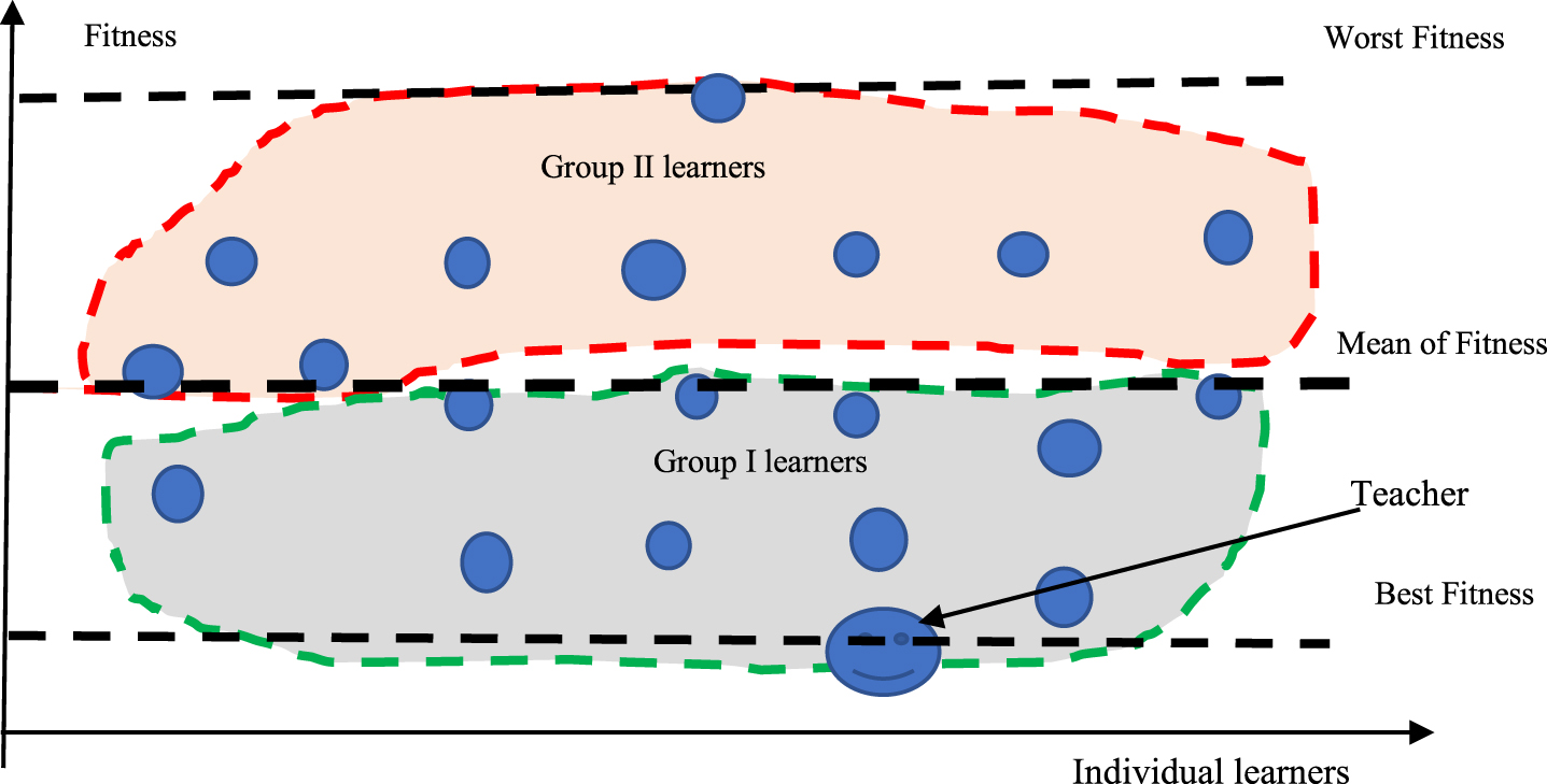
Grouping method based on performance (for min objective).

In Fig. 2, we divide the class students into two groups: G (I) = {i : |Fitness_best ⩽ Fitness_i < Fitness_mean}, and G (II) = {i : |Fitness_mean ⩽ Fitness_i ⩽ Fitness_worst}.

Based on the grouping results, the teaching operators are described as follows.

Case I: if one individual i ∈ G (I) $\begin{matrix} X_{i}^{new} = X_{i} + w_{1} * \vec{R} \otimes {(X_{Teacher} - T_{f} * X_{i}} \\ + w_{2} * \vec{R} \otimes {X_{Teacher} - T_{f} * X_{mean}}, \end{matrix}$ (22)

Case II: if one individual i ∈ G (II) $\begin{matrix} X_{i}^{new} = X_{mean} + w_{1} * \vec{R} \otimes {(X_{mean} - T_{f} * X_{i}} \\ + w_{2} * \vec{R} \otimes {X_{Teacher} - T_{f} * X_{mean}}, \end{matrix}$ (23) where w₁, w₂ are weight factors and set them as 0.5.

For learners of group I after teaching process, the basic idea of this operator is that their knowledge level should look up to the teacher, but for learners of group II, their knowledge level should look up to the mean level.

3.3 Learning phase

In this paper, we divide the learning phase into two steps, the first step is called multi-point neighbor learning (MPNL), this operator changes the two-neighbor learning strategy of the original TLBO to a three-neighbor learning strategy. The second step is a mixed self-learning operator (MSL) composed of two selective operators depending a random, i.e., mixed learning of self-learning and inter-learning (MLSI), mixed learning of self-learning and team learning (MLST).

(1) Multi-point neighbor learning operator (MPNL)

In this operator, the way of a learner gains knowledge has two choices depending on a random number. If the random number is larger than a given number, the learner gains knowledge from interaction with a random selected neighbor, otherwise, she(he) will gain knowledge from interaction with other two randomly selected neighbors.

Case I: if rand)>0.5

Randomly select a neighbor of individual learner i, X_Partner(i) ≠ i. Update the solution of individual i as follows. $\begin{matrix} X_{i}^{new} = \\ {\begin{matrix} X_{i} + \vec{R} \otimes {X_{i} - X_{Partner (i)}}, if F (X_{i}) < F (X_{Partner (i)}) \\ X_{i} + \vec{R} \otimes {X_{Partner (i)} - X_{i}}, otherwise \end{matrix} \end{matrix}$ (24)

Case II: Otherwise (rand< =0.5)

Randomly select two neighbors $X_{Partner (i)}^{1}$ and $X_{Partner (i)}^{2}$ , $X_{Partner (i)}^{1} \neq X_{Partner (i)}^{2} \neq X_{i}$ . Update the solution of individual i and follows.

If $F (X_{i}) < F (X_{Partner (i)}^{1})$ and $F (X_{Partner (i)}^{1}) < F (X_{Partner (i)}^{2})$ $\begin{matrix} X_{i}^{new} = X_{i} + \vec{R} \otimes {X_{i} - X_{Partner (i)}^{1}} \\ + \vec{R} \otimes {X_{Partner (i)}^{1} - X_{Partner (i)}^{2}}, \end{matrix}$ (25) Otherwise $\begin{matrix} X_{i}^{new} = X_{i} + \vec{R} \otimes {X_{Partner (i)}^{1} - X_{i}} + \\ \vec{R} \otimes {X_{Partner (i)}^{2} - X_{Partner (i)}^{1}} . \end{matrix}$ (26)

(2) Mixed Self-learning operator (MSL)

In addition to the multi-point learning mechanism, two self-learning operators are also developed in learning phase, i.e., MLSI (mixed learning of self-learning with inter-learning) and MLSI (mixed learning of self-learning with team-learning).

First: calculate the mean solution of learner i during the last three iterations before current iteration t using the following equation: $X_{mean}^{i} = (I X_{i} (t - 1) + I X_{i} (t - 2) + I X_{i} (t - 3)) / 3,$ (27) where IX_i (t) = X_i.

Algorithm of CTLBO: Pseudo code of CTLBO
	/Initialization of algorithm parameters/
	Set the population size NP, Dimension D, iteration T_max, lower and upper limit of the problem, [L_b,U_b].
01:	Fori = 1 to NP do
02:	Randomly generate individual solution Xi according to (2)
03:	Calculate Fi = F(Xi)
04:	End for
05:	Y = X;
06:	Set parameters for TLI operator: c₁₀=0.5; c₂₀=0.25; w₁₀=0.5;q₀=0.5;
	/* enter iteration*/
07:	Fort = 1 to T_maxdo
08:	E = 2*(1-t/T_max);
09:	TSL₁=2/(1 + exp(1-t/T_max));
10:	Fori = 1 to NP do
11:	Determine the best solution of population size as the teacher
12:	$X_{Teacher} = \underset{i}{argmin} (f (x_{1}), f (x_{2}, \dots, f (x_{NP}))$ and the mean of the population: $X_{mean} = \frac{1}{NP} \sum_{i = 1}^{NP} X_{i}$
	/TLI operator (Teacher-learner interaction) /
13:	w₁₀ = w₁₀(1-t/T_max); c₁₀=c₁₀(1-t/(t+T_max));
14:	c₂₀=c₂₀(1 + t/T_max); q=q₀(1- t/T_max)
15:	Using equation (5) and (6) to calculate the velocity and position
16:	Evaluate fitness F(Y_i);
17:	If F (Y_i)<F (X_i)then
18:	X_i = Y_i, F (X_i) = F (Y_i)
19:	Endif
	/* TSL operator (teacher self-learning) */
20:	L₀=2*rand (0, 1)-1;
21	L_v=E*L₀;
22:	TSL₂=2*(1-rand (0, 1));
23:	Ift > 2then
24:	According to Eq. (16) to update the teacher’s knowledge
25:
26:	Calculate F_{new_teacher}=F ( $X_{Teacher}^{new}$ )
27:	IfF_{new_teacher}< F (X_Teacher) then
28:	X_Teacher= $X_{Teacher}^{new}$ , F (X_Teacher)=F_{new_teacher}
29:	Endif
	Endif
30:	/begin teaching phase/
	T_f = round (1 + rand (0, 1)) /*teaching factor generating
31:	/MCT operator of teaching phase /
32:	If rand > 0.5 then
33:	Update $X_{i}^{new}$ using Eq. (17);
34:	Else
35:	Update $X_{i}^{new}$ using Eq. (18);
36:	Endif
37:	Calculate the fitness F ( $X_{i}^{new}$ )
38:	If $F (X_{i}^{new}) < F (X_{i})$ then
39:	$X_{i} = X_{i}^{new}$ , $F (X_{i}) = F (X_{i}^{new})$ .
	Endif
40:	/PBGT operator of teaching phase /
41:	Classify students into two groups G(I) and G(II) according to:
42:	G (I) = {i : \|Fitness_best⩽ Fitness_i <,
43:	Fitness_mean}, and G (II) = {i : \|Fitness_mean⩽.
44:	Fitness_i ⩽ Fitness_worst}
45:	If i∈G(I) then
46:	Update $X_{i}^{new}$ using Eq. (22);
47:	Else % % (i∈G(II))
48:	Update $X_{i}^{new}$ using Eq. (23);
49:	Endif
50:	Calculate the fitness F ( $X_{i}^{new}$ )
51:	If $F (X_{i}^{new}) < F (X_{i})$ then
52:	$X_{i} = X_{i}^{new}$ , $F (X_{i}) = F (X_{i}^{new})$ .
53:	Endif
	/* neighbor learning phase with MPNL operator */
54:	If rand > 0.5 then
55:	Select one neighbor of i, X_Parrtner(i)
56:	Update $X_{i}^{new}$ using Eq. (24);
57:	Else
58:	Select two neighbors of i, $X_{Partner (i)}^{1}$ and $X_{Partner (i)}^{2}$
59:	Update $X_{i}^{new}$ using Eq. (25) and (26);
60:	Endif
61:	Calculate the fitness F ( $X_{i}^{new}$ )
62:	If $F (X_{i}^{new}) < F (X_{i})$ then
63:	$X_{i} = X_{i}^{new}$ , $F (X_{i}) = F (X_{i}^{new})$ .
64:	Endif
65:	/* Mixed self-learning phase */
66:	If iteration< =3then
67:	μ = L_b + U_b - X_i
68:	If rand > 0.5 then
69:	$X_{i}^{new} = X_{i} + rand (0, 1) * abs (rand (0, 1) * μ - X_{i})$
70:	Else
71:	$X_{i}^{new} = X_{i} - rand (0, 1) * abs (rand (0, 1) * μ - X_{i})$
72:	Endif
73:	Calculate the fitness F ( $X_{i}^{new}$ )
74:	If $F (X_{i}^{new}) < F (X_{i})$ then
	$X_{i} = X_{i}^{new}$ , $F (X_{i}) = F (X_{i}^{new})$ .
75:	Endif
76:	Else /when iteration > 3/
77:	Calculate the mean of i^th with the last three iterations using Eq. (27)
78:	If rand > 0.5, then
79:	Execute the MLSL operator using Eq. (28-30)
80:	Else
81:	Execute MLST operator using Eq. (31-34)
82:	Endif
83:	Calculate the fitness F ( $X_{i}^{new}$ )
84:	If $F (X_{i}^{new}) < F (X_{i})$ then
85:	$X_{i} = X_{i}^{new}$ , $F (X_{i}) = F (X_{i}^{new})$ .
86:	Endif
87:	Endif
88:	End for /* end of population size i*/
89:	Record the global optimal solution of iteration t
90:	GG(t) and F(X);
91:	End for /* end of iteration t*/
	Output optimal solution
	X^* = argmin F (X) , F^* = min (F (X))

Case I: if rand > 0.5, execute MLSI operator $\begin{matrix} X_{i}^{new - 1} = X_{i} + 2 * (1 - \frac{t}{T_{\max}}) * 1 + cos (\frac{i}{NP}) \\ * \vec{R} \otimes {X_{i} - I X_{i} (t - 1)} \end{matrix}$ (28) $\begin{matrix} X_{i}^{new - 2} = X_{i} + 2 * (1 - \frac{t}{T_{\max}}) * 1 + cos (\frac{i}{NP}) \\ * \vec{R} \otimes {X_{Partner (i)}^{□} - X_{mean}^{i}} \end{matrix}$ (29) $X_{i}^{new} = s_{1} * X_{i}^{new - 1} + s_{2} * X_{i}^{new - 2}$ (30) where s₁ = 0.5, s₂ = 0.5.

Case II: else execute MLST operator $\begin{matrix} X_{i}^{new - 1} = X_{i} + 2 * (1 - \frac{t}{T_{\max}}) * 1 + \sin (\frac{i}{NP}) \\ * \vec{R} \otimes {X_{i} - I X_{i} (t - 1)} \end{matrix}$ (31) $\begin{matrix} X_{i}^{new - 2} = X_{i} + 2 * (1 - \frac{t}{T_{\max}}) * 1 + \cos (\frac{i}{NP}) \\ * \vec{R} \otimes {X_{mean} - X_{mean}^{i})} \end{matrix}$ (32) $\begin{matrix} X_{i}^{new - 3} = X_{i} + 2 * (1 - \frac{t}{T_{\max}}) * 1 + \cos (\frac{i}{NP}) \\ * \vec{R} \otimes {X_{Partner (i)} - X_{mean}^{i})} \end{matrix}$ (33)

$X_{i}^{new} = s_{3} * X_{i}^{new - 1} + s_{4} * X_{i}^{new - 2} + s_{5} * X_{i}^{new - 3}$ (34) where s₃ = 0.5, s₄ = 0.3, s₅ = 0.2.

Above self-learning operators are executed when the iteration is larger than 3, i.e. t > 3. The pseudo code of CTLBO algorithm is described in the followings.

4 Experiment and analysis

In order to illustrate the effectiveness of CTLBO algorithm, two sets of experiments are conducted. The first set of experiments validate the improvement effect of CTLBO by comparing with the original version of TLBO. The second set of experiments illustrate the advantage of CTLBO by comparing it with other 9 state-of-the-art algorithms in solving 30 general benchmark functions.

During experiments in this paper, all algorithms are coded in MATLAB and tested in Windows 10 on a PC with Core (TM) i7-7500U CPU 2.70 GHz, 8GB RAM.

4.1 Improvement effect validation of CTLBO

In this section, we conduct four experiments to illustrate the advantage of CTLBO. Experiment A is to compare CTLBO with original TLBO, the other three experiments–B, C, and D, are to compare CTLBO with other versions of improved TLBO reported in literature.

4.1.2 Experiment A–comparison with original TLBO

(1) Benchmark functions

In this section, 15 benchmark functions are selected as comparison base. Those functions are very representative and most of them have been widely tested in other research literature, which have generalized comparison value for algorithm research. Those 15 functions are divided into two groups: (1) 6 unimodal functions: Dixon-price, Quartic, Rosenbrock, Sphere, Sum-squares, Zakharov, and (2) 9 multimodal functions: Ackley, Alpine, Exponential, Generalized-Penalized function 1 (Generalized), Griewank, Michalewics, Rastrigin, Schwefel, and Shaffer7. The detail function characteristics: function expressions, solution ranges, optimal solutions are listed in Appendix A. In order to compare the algorithm stability and effectiveness in solving different scale problems, we conduct experiments with different dimensions for five scales: Dim = 100, 300, 1000, 3000, 5000 for all functions. The algorithm parameters for TLBO and CTLBO are set as: the population size = 50, the maximal iteration = 500. For all functions, the two algorithms run 30 times.

(2) Results and analysis

We compare all functions with “mean”, “standard deviation (STD)” for each function and dimension. Results are listed as Table 1. From the results of Table 1, CTLBO algorithm can obtain significant improvement in all benchmark functions.

Table 1
Experiment A-Comparison of CTLBO with TLBO on high dimensional general functions (population size = 50, iteration 500)

Function Dim=100 Dim=300 Dim=1000 Dim=3000 Dim=5000

Best Mean STD Best Mean STD Best Mean STD Best Mean STD Best Mean STD

Ackley TLBO 7.99E-15 0.126547 0.693128 7.99E-15 0.47705 1.455693 7.99E-15 3.897393 3.604640 7.99E-15 6.535661 3.170354 5.720433 9.969923 2.367327

CTLBO 8.88E-16 8.88E-16 0 8.88E-16 8.88E-16 0 8.88E-16 8.88E-16 0 8.88E-16 8.88E-16 0 8.88E-16 8.88E-16 0

Alpine TLBO 4.22E-38 8.53E-38 4.1E-38 4.26E-37 1.01E-36 3.11E-37 1.86E-36 5.58E-36 2.27E-36 6.91E-36 2.04E-35 8.33E-36 1.76E-35 3.7E-35 1.34E-35

CTLBO 0 0 0 0 0 0 0 0 0 0 0 0 0 0 0

Dixon_price TLBO 6.67E-01 6.67E-01 3.39E-16 6.67E-01 6.67E-01 3.39E-16 6.67E-01 6.67E-01 4.03E-08 6.67E-01 6.67E-01 6.48E-08 6.67E-01 6.67E-01 1.83E-08

CTLBO 2.55E-03 2.22E-02 1.69E-02 7.61E-02 1.63E-01 4.91E-02 1.67E-01 1.90E-01 3.58E-02 1.67E-01 2.21E-01 1.25E-01 1.67E-01 3.62E-01 2.37E-01

Exponential TLBO 0 0 0 0 0 0 0 0 0 0 0 0 0 0 0

CTLBO -1 -1 0 -1 -1 0 -1 -1 0 -1 -1 0 -1 -1 0

Griewank TLBO 0 0 0 0 0 0 1.11E-16 1.11E-16 2.51E-32 1.11E-16 1.11E-16 2.51E-32 1.11E-16 1.11E-16 2.51E-32

CTLBO 0 0 0 0 0 0 0 0 0 0 0 0 0 0 0

Generalized TLBO 0.00188 0.005481 0.002794 0.11006 0.137513 0.015839 0.510016 0.545383 0.013794 0.84569 0.87122 0.012189 0.93838 0.968717 0.009563

CTLBO 1.28E-12 1.32E-10 2.32E-10 3.05E-12 3.05E-09 7.84E-09 1.1E-12 6.14E-09 1.06E-08 1.62E-13 9.68E-09 1.83E-08 1.6E-11 4.73E-09 7.3E-09

Michalewics TLBO -36.4367 -32.5345 1.750933 -77.3843 -73.5275 2.012325 -219.409 -210.328 2.82209 -593.177 -581.124 4.886076 -955.415 -943.661 5.40097

CTLBO -74.5963 -44.6683 10.38998 -120.055 -119.117 0.716587 -397.841 -391.641 26.82029 -1193.54 -1131.44 148.5865 -1989.13 -1711.65 344.181

Quartic TLBO 7.28E-04 1.38E-03 4.28E-04 1.65E-03 8.78E-04 5.39E-04 9.17E-04 1.70E-03 5.23E-04 8.03E-04 1.88E-03 5.38E-04 1.27E-03 2.01E-03 4.20E-04

CTLBO 2.23E-06 5.69E-05 3.96E-05 5.79E-06 6.09E-05 3.48E-05 3.71E-06 5.65E-05 4.35E-05 5.42E-06 6.92E-05 4.43E-05 3.06E-06 6.67E-05 3.81E-05

Rastrigin TLBO 0 0 0 0 0 0 0 0 0 0 0 0 0 0 0

CTLBO 0 0 0 0 0 0 0 0 0 0 0 0 0 0 0

Rosenbrock TLBO 92.61684 94.5399 1.096539 294.2257 296.095 0.971994 994.1986 995.7962 0.373291 2994.422 2995.05 0.211916 4994.161 4994.703 0.182062

CTLBO 7.31E-08 5.85E-06 1.08E-05 5.94E-08 2.02E-04 4.76E-04 1.07E-06 2.73E-03 7.93E-03 4.97E-07 1.40E-02 3.38E-02 7.8E-06 8.72E-03 1.91E-02

Schwefle TLBO 14708.02 24241.75 4598.353 71665.85 90947.56 12544.89 303372.3 363020.5 24367.74 1039567 1126071 53839.01 1821180 1939744 59645.68

CTLBO 8.02E-01 5.07E+03 5.75E+03 3.99E+02 3.00E+04 2.13E+04 1.26E+03 9.00E+04 9.30E+04 3.49E+03 3.20E+05 2.68E+05 1.74E+04 3.25E+05 3.61E+05

Shaffer7 TLBO 1.776764 15.27621 11.276 0.356545 1.408581 1.470319 5.942101 7.299882 0.527842 34.13893 36.38465 1.004079 66.74088 70.43767 1.82966

CTLBO 0 2.59E-16 8.47E-16 0 3.6E-14 1.49E-13 0 3.57E-17 9.81E-17 0 2.29E-13 1.05E-12 0 6.25E-14 3.27E-13

Sphere TLBO 1.06E-73 5.06E-73 3.63E-73 2.38E-71 1.63E-70 1.2E-70 5.3E-70 4.06E-69 3.12E-69 1.41E-68 5.24E-68 3.26E-68 3.11E-68 1.02E-67 6.65E-68

CTLBO 0 0 0 0 0 0 0 0 0 0 0 0 0 0 0

Sum_square TLBO 1.81E-74 1.8E-73 1.65E-73 1.39E-71 2.94E-70 3.83E-70 1.98E-69 2.58E-68 2.04E-68 8.64E-68 5.1E-67 7.35E-67 4.27E-67 2.08E-66 2.13E-66

CTLBO 0 0 0 0 0 0 0 0 0 0 0 0 0 0 0

Zakharov TLBO 56.58768 102.9749 20.55557 528.8424 996.3924 195.8438 1835.012 3357.645 689.0827 6277.548 11045.57 2777.583 11038.55 19898.26 8237.109

CTLBO 0 0 0 0 0 0 0 0 0 0 0 0 0 0 0

Function	Dim=100	Dim=300	Dim=1000	Dim=3000	Dim=5000
Ackley	TLBO	7.99E-15	0.126547	0.693128	7.99E-15	0.47705	1.455693	7.99E-15	3.897393	3.604640	7.99E-15	6.535661	3.170354	5.720433	9.969923	2.367327
	CTLBO	8.88E-16	8.88E-16	0	8.88E-16	8.88E-16	0	8.88E-16	8.88E-16	0	8.88E-16	8.88E-16	0	8.88E-16	8.88E-16	0
Alpine	TLBO	4.22E-38	8.53E-38	4.1E-38	4.26E-37	1.01E-36	3.11E-37	1.86E-36	5.58E-36	2.27E-36	6.91E-36	2.04E-35	8.33E-36	1.76E-35	3.7E-35	1.34E-35
	CTLBO	0	0	0	0	0	0	0	0	0	0	0	0	0	0	0
Dixon_price	TLBO	6.67E-01	6.67E-01	3.39E-16	6.67E-01	6.67E-01	3.39E-16	6.67E-01	6.67E-01	4.03E-08	6.67E-01	6.67E-01	6.48E-08	6.67E-01	6.67E-01	1.83E-08
	CTLBO	2.55E-03	2.22E-02	1.69E-02	7.61E-02	1.63E-01	4.91E-02	1.67E-01	1.90E-01	3.58E-02	1.67E-01	2.21E-01	1.25E-01	1.67E-01	3.62E-01	2.37E-01
Exponential	TLBO	0	0	0	0	0	0	0	0	0	0	0	0	0	0	0
	CTLBO	-1	-1	0	-1	-1	0	-1	-1	0	-1	-1	0	-1	-1	0
Griewank	TLBO	0	0	0	0	0	0	1.11E-16	1.11E-16	2.51E-32	1.11E-16	1.11E-16	2.51E-32	1.11E-16	1.11E-16	2.51E-32
	CTLBO	0	0	0	0	0	0	0	0	0	0	0	0	0	0	0
Generalized	TLBO	0.00188	0.005481	0.002794	0.11006	0.137513	0.015839	0.510016	0.545383	0.013794	0.84569	0.87122	0.012189	0.93838	0.968717	0.009563
	CTLBO	1.28E-12	1.32E-10	2.32E-10	3.05E-12	3.05E-09	7.84E-09	1.1E-12	6.14E-09	1.06E-08	1.62E-13	9.68E-09	1.83E-08	1.6E-11	4.73E-09	7.3E-09
Michalewics	TLBO	-36.4367	-32.5345	1.750933	-77.3843	-73.5275	2.012325	-219.409	-210.328	2.82209	-593.177	-581.124	4.886076	-955.415	-943.661	5.40097
	CTLBO	-74.5963	-44.6683	10.38998	-120.055	-119.117	0.716587	-397.841	-391.641	26.82029	-1193.54	-1131.44	148.5865	-1989.13	-1711.65	344.181
Quartic	TLBO	7.28E-04	1.38E-03	4.28E-04	1.65E-03	8.78E-04	5.39E-04	9.17E-04	1.70E-03	5.23E-04	8.03E-04	1.88E-03	5.38E-04	1.27E-03	2.01E-03	4.20E-04
	CTLBO	2.23E-06	5.69E-05	3.96E-05	5.79E-06	6.09E-05	3.48E-05	3.71E-06	5.65E-05	4.35E-05	5.42E-06	6.92E-05	4.43E-05	3.06E-06	6.67E-05	3.81E-05
Rastrigin	TLBO	0	0	0	0	0	0	0	0	0	0	0	0	0	0	0
	CTLBO	0	0	0	0	0	0	0	0	0	0	0	0	0	0	0
Rosenbrock	TLBO	92.61684	94.5399	1.096539	294.2257	296.095	0.971994	994.1986	995.7962	0.373291	2994.422	2995.05	0.211916	4994.161	4994.703	0.182062
	CTLBO	7.31E-08	5.85E-06	1.08E-05	5.94E-08	2.02E-04	4.76E-04	1.07E-06	2.73E-03	7.93E-03	4.97E-07	1.40E-02	3.38E-02	7.8E-06	8.72E-03	1.91E-02
Schwefle	TLBO	14708.02	24241.75	4598.353	71665.85	90947.56	12544.89	303372.3	363020.5	24367.74	1039567	1126071	53839.01	1821180	1939744	59645.68
	CTLBO	8.02E-01	5.07E+03	5.75E+03	3.99E+02	3.00E+04	2.13E+04	1.26E+03	9.00E+04	9.30E+04	3.49E+03	3.20E+05	2.68E+05	1.74E+04	3.25E+05	3.61E+05
Shaffer7	TLBO	1.776764	15.27621	11.276	0.356545	1.408581	1.470319	5.942101	7.299882	0.527842	34.13893	36.38465	1.004079	66.74088	70.43767	1.82966
	CTLBO	0	2.59E-16	8.47E-16	0	3.6E-14	1.49E-13	0	3.57E-17	9.81E-17	0	2.29E-13	1.05E-12	0	6.25E-14	3.27E-13
Sphere	TLBO	1.06E-73	5.06E-73	3.63E-73	2.38E-71	1.63E-70	1.2E-70	5.3E-70	4.06E-69	3.12E-69	1.41E-68	5.24E-68	3.26E-68	3.11E-68	1.02E-67	6.65E-68
	CTLBO	0	0	0	0	0	0	0	0	0	0	0	0	0	0	0
Sum_square	TLBO	1.81E-74	1.8E-73	1.65E-73	1.39E-71	2.94E-70	3.83E-70	1.98E-69	2.58E-68	2.04E-68	8.64E-68	5.1E-67	7.35E-67	4.27E-67	2.08E-66	2.13E-66
	CTLBO	0	0	0	0	0	0	0	0	0	0	0	0	0	0	0
Zakharov	TLBO	56.58768	102.9749	20.55557	528.8424	996.3924	195.8438	1835.012	3357.645	689.0827	6277.548	11045.57	2777.583	11038.55	19898.26	8237.109
	CTLBO	0	0	0	0	0	0	0	0	0	0	0	0	0	0	0

For the accuracy (best solutions and average solutions), CTLBO are far better than TLBO on all 15 benchmark functions. Based on the results of Table 1, we find for CTLBO, there are 8 functions have 100% (percent rate 53% of all functions) to obtain 100% optimal solution for all dimensions, but TLBO has only one function (6%) can 100% obtain optimal for all dimension. For the stability, except for three functions: Dixon-price, Michalewics and Schwefel, all other 13 functions, CLTBO can outperform TLBO. Based on the results of Table 1, we can summarize the following conclusion: CTLBO can obtain improvement effect for all benchmark functions than TLBO on best and average solutions.

On the other hand, from the comparison of different dimensional functions, Fig. 3 shows the comparison results of selected functions. It can be seen that for different functions, with the increase of dimension, the accuracy of CTLBO can remain relative stable, but TLBO accuracy deteriorates fast with the increase of dimension. Therefore, we can summarize that for large scale optimization problems, with the increase of dimensions, for most benchmark functions, accuracies of TLBO will fast deteriorate, while CTLBO can remain high accuracies for all high dimensional functions. This reveals that CTLBO can more effectively solve large scale problems than TLBO.

Fig. 3

Fitnesses of CTLBO vs TLBO for selected functions on different dimensions.

4.1.3 Comparison with other improved versions of TLBO algorithm

Experiment B: In this experiment, there are 10 benchmark functions and 5 other compared improved versions of TLBO algorithm, which are reported by the literature Zuo et al. [8]. The results are listed in Table 2. The algorithm population size = 50, FEs = 300, 000; the dimension of all functions is 30; for all functions, each algorithm is run 30 times.

Table 2
Experiment B–comparison of CTLBO with other variants of TLBO

Function Results TLBO ETLBO NSTLBO I-TLBO DRLTLBO CTLBO

(Rao, et al. [11]) (Rao and Patel [25]) (Wang et al. [43]) (Ji et al. [17]) (Zuo et al. [8]) (this paper)

Ackley Mean 3.55e-015 3.55e-015 3.55e-015 3.55e-015 3.55e-015 8.88e-16

Std 0 0 0 0 0 0

Rank 2 2 2 2 2 1

Griewank Mean 0 0 0 0 0 0

Std 0 0 0 0 0 0

Rank 1 1 1 1 1 1

Quadric Mean 8.61e-122 1.89e-118 2.58e-265 2.62e-050 4.26e-288 0

Std 1.44e-121 3.10e-118 4.32e-266 3.29e-050 1.18e-289 0

Rank 4 5 3 6 2 1

Rastrigin Mean 9.29e+000 9.95e+000 0 3.26e+001 1.86e+001 0

Std 3.03e+000 8.50e+000 0 1.16e+001 1.84e+001 0

Rank 2 3 1 5 4 1

Rosenbrock Mean 1.05e+001 7.42e+000 2.26e+001 5.80e+000 3.98e-012 2.45e-014

Std 8.86e-001 1.69e+000 1.17e-001 6.05e+000 6.58e-012 7.10e-014

Rank 5 4 6 3 2 1

Schewefel Mean 4.06e+003 3.88e+003 4.19e+003 3.73e+003 3.77e+003 1.08e+003

Std 4.44e+002 2.69e+002 6.07e+002 3.27e+002 1.07e+003 9.00e+002

Rank 5 4 6 2 3 1

Sphere Mean 0 0 0 7.56e-258 0 0

Std 0 0 0 2.83e-258 0 0

Rank 1 1 1 2 1 1

Sum Square Mean 0 0 0 9.87e-259 0 0

Std 0 0 0 2.75e-259 0 0

Rank 1 1 1 2 1 1

Weierstrass Mean 0 0 0 0 0 0

Std 0 0 0 0 0 0

Rank 1 1 1 1 1 1

Zakharov Mean 3.55e-080 5.22e-078 9.29e-150 1.15e-033 6.66e-275 0

Std 2.28e-080 3.11e-078 9.70e-150 1.02e-033 1.48e-276 0

Rank 4 5 3 6 2 1

Function	Results	TLBO	ETLBO	NSTLBO	I-TLBO	DRLTLBO	CTLBO
Ackley	Mean	3.55e-015	3.55e-015	3.55e-015	3.55e-015	3.55e-015	8.88e-16
	Std	0	0	0	0	0	0
	Rank	2	2	2	2	2	1
Griewank	Mean	0	0	0	0	0	0
	Std	0	0	0	0	0	0
	Rank	1	1	1	1	1	1
Quadric	Mean	8.61e-122	1.89e-118	2.58e-265	2.62e-050	4.26e-288	0
	Std	1.44e-121	3.10e-118	4.32e-266	3.29e-050	1.18e-289	0
	Rank	4	5	3	6	2	1
Rastrigin	Mean	9.29e+000	9.95e+000	0	3.26e+001	1.86e+001	0
	Std	3.03e+000	8.50e+000	0	1.16e+001	1.84e+001	0
	Rank	2	3	1	5	4	1
Rosenbrock	Mean	1.05e+001	7.42e+000	2.26e+001	5.80e+000	3.98e-012	2.45e-014
	Std	8.86e-001	1.69e+000	1.17e-001	6.05e+000	6.58e-012	7.10e-014
	Rank	5	4	6	3	2	1
Schewefel	Mean	4.06e+003	3.88e+003	4.19e+003	3.73e+003	3.77e+003	1.08e+003
	Std	4.44e+002	2.69e+002	6.07e+002	3.27e+002	1.07e+003	9.00e+002
	Rank	5	4	6	2	3	1
Sphere	Mean	0	0	0	7.56e-258	0	0
	Std	0	0	0	2.83e-258	0	0
	Rank	1	1	1	2	1	1
Sum Square	Mean	0	0	0	9.87e-259	0	0
	Std	0	0	0	2.75e-259	0	0
	Rank	1	1	1	2	1	1
Weierstrass	Mean	0	0	0	0	0	0
	Std	0	0	0	0	0	0
	Rank	1	1	1	1	1	1
Zakharov	Mean	3.55e-080	5.22e-078	9.29e-150	1.15e-033	6.66e-275	0
	Std	2.28e-080	3.11e-078	9.70e-150	1.02e-033	1.48e-276	0
	Rank	4	5	3	6	2	1

Note: The algorithm parameters of CTLBO are set as Zuo et al. [8]), population size = 50, FEs = 300000. D = 30dimensions.

In this experiment, the average ranks for all compared algorithms are: CTLBO = 1, DRLTLBO = 1.7, I-TLBO=3, NSTLBO = 2.5, ETLBO = 2.7, TLBO =2.6. according to ranks, the sequence of comparison advantages of these algorithms is: CTLBO (1) ≻ DRLTLBO (1.7) ≻ NSLTLBO (2.5) ≻ TLBO (2.6) ≻ ETLBO (2.7). Furthermore, from this experiment, we know the success rate of 100% obtaining optimal solution for CTLBO is 80%. NSTLBO is 50%, DRTLBO, TBLO, ETLBO are 40%, I-TLBO is 20%

Example C: In this experiment, we compared our CTLBO algorithm with improved versions of TLBO algorithm of literature Xu et al. [19]. There are 11 benchmark functions and 5 compared algorithms of other variants of improved TBLO. The results are listed in Table 3. The algorithm population size is 100, function evaluation number is FEs = 300, 000, the dimension of all functions is 30, and for all functions, each algorithm is run 30 times.

Table 3

Experiment C–comparison of CTLBO with other variants of TLBO

Function	Results	SLTLBO	ETLBO	MTLBO	OTLBO	DOLTLBO	CTLBO
		(Yang et al. [26])	(Kadambur [44])	(Sataptathy et al. [45])	(Roy et al. [46])	(Xu et al. [19])	(this paper)
Ackley	Mean	2.05E+01	2.09E+01	2.03E+01	2.05E+01	2.04E+01	8.88E-16
	Std	1.30E-01	8.41E-02	1.04E-01	1.15E-01	1.51E-01	0
	Rank	5	6	2	4	3	1
Bent Cigar	Mean	1.88E+10	2.12E+10	2.77E+10	3.87E+03	1.09E+03	0
	Std	5.48E+09	5.54E+09	7.94E+09	4.69E+03	5.89E+03	0
	Rank	4	5	6	3	2	1
Discus	Mean	3.94E+04	5.11E+04	6.79E+04	7.46E+02	5.48E-03	0
	Std	1.05E+04	1.45E+04	1.53E+04	8.35E+02	1.10E-02	0
	Rank	4	5	6	3	2	1
Griewank	Mean	1.50E+02	1.50E+02	2.13E+02	3.97E-02	2.00E-01	0
	Std	4.04E+01	4.00E+01	5.19E+01	5.35E-02	3.22E-01	0
	Rank	4	5	6	2	3	1
Happy Cat	Mean	3.46E+00	3.94E+00	4.31E+00	7.70E-01	5.18E-01	8.07E-02
	Std	6.00E-01	4.42E-01	5.94E-01	1.24E-01	1.04E-01	3.27E-02
	Rank	4	5	6	3	2	1
HGBat	Mean	5.16E+01	5.95E+01	7.72E+01	5.58E-01	5.05E-01	1.84E-01
	Std	1.71E+01	1.85E+01	1.70E+01	3.26E-01	2.60E-01	2.03E-01
	Rank	4	5	6	3	2	1
High conditioned elliptic	Mean	9.74E+07	1.57E+08	2.32E+08	4.64E+05	6.08E+04	0
	Std	3.99E+07	6.50E+07	8.50E+07	2.42E+05	5.22E+04	0
	Rank	4	5	6	3	2	1
Katsuura	Mean	1.86E+00	3.80E+00	2.34E+00	1.59E+00	1.56E+00	0
	Std	7.09E-01	1.36E+00	8.09E-01	6.22E-01	5.47E-01	0
	Rank	4	6	5	3	2	1
Rastrigin	Mean	2.22E+02	2.55E+02	2.69E+02	1.20E+02	1.11E+02	0
	Std	3.34E+01	2.64E-01	3.41E+01	2.12E+01	2.00E+01	0
	Rank	4	5	6	3	2	1
Rosenbrock	Mean	1.15E+03	1.39E+03	1.96E+03	3.04E+01	2.53E+01	1.27E-11
	Std	4.96E+02	7.74E+02	7.37E+02	1.34E+01	2.12E+00	5.21E-11
	Rank	4	5	6	3	2	1
Weierstrass	Mean	5.59E+01	6.61E+01	6.79E+01	5.52E+01	4.95E+01	0
	Std	2.00E+01	2.42E+01	2.37E+01	1.97E+01	1.82E+01	0
	Rank	4	5	6	3	2	1

Note: The algorithm parameters of CTLBO are set as Xu et al. [19]. Population size = 100, FES = 300, 000. D = 30dimension.

From this experiment, the total average ranks: CTLBO = 1, DOLTLBO = 2.18, OTLBO = 3, MTLBO = 5.55, ETLBO = 5.18, SLTLBO = 4.09. According to order of ranks, the sequence of comparison advantage is: $\begin{matrix} CTLBO (1) ≻ DOLTLBO (2.18) ≻ OTLBO (3) ≻ \\ SLTLBO (4.09) ≻ ETLBO (5.18) ≻ MTLBO (5.55) \end{matrix}$

Furthermore, from this experiment, we know the success rate of 100% obtaining optimal solution for CTLBO is 72%.; all other algorithms are 0%.

Experiment D: In this experiment, we compared our CTLBO algorithm with improved versions of TLBO algorithm of literature Wu et al. [10]. There are 9 benchmark functions and 4 compared algorithms of other variants of improved TBLO. The results are listed in Table 4. The algorithm population size is 30, function evaluation number is FEs = 300, 000, the dimension of all functions is 30, and for all functions, the algorithm is run 30 times.

Table 4

Experiment D–comparison of CTLBO with other variants of TLBO

Function	Results	LETLBO	ITLBO	I-TLBO	DI-TLBO	CTLBO
		(Zuo et al. [47])	(Yu et al. [48])	(Ji et al. [17])	(Wu et al. [10])	(this paper)
Dixon-price	Mean	6.67E-01	6.67E-01	6.67E-01	6.67E-01	7.91E-10
	Std	3.58E–16	6.10E-12	9.29E-17	1.68E-17	1.26E-09
	Rank	4	5	3	2	1
Griewank	Mean	0	0	0	0	0
	Std	0	0	0	0	0
	Rank	1	1	1	1	1
Quardric	Mean	0	3.40E-256	1.07E-113	3.82E-125	0
	Std	0	0.00E+00	3.21E-113	1.23E-124	0
	Rank	1	2	4	3	1
Penalized 2	Mean	3.22E-02	8.55E-02	1.95E-02	1.05E-02	1.63E-21
	Std	6.56E-02	6.64E-02	3.89E-02	3.15E-02	6.91E-21
	Rank	4	5	3	2	1
Rastrigin	Mean	0	21.6E+01	0	0	0
	Std	0	1.54E+01	0	0	0
	Rank	1	2	1	1	1
Schwefel	Mean	4.62E+03	4.49E+03	3.32E+02	3.08E+02	1.32E+03
	Std	6.39E+02	6.23E+02	1.58E+02	1.67E+02	1.47E+03
	Rank	5	4	2	1	3
Sphere	Mean	0	0	0	0	0
	Std	0	0	0	0	0
	Rank	1	1	1	1	1
Sum Squares	Mean	0	0	0	0	0
	Std	0	0	0	0	0
	Rank	1	1	1	1	1
Zakharov	Mean	1.10E-280	2.84E-174	1.09E-84	1.05E-86	0
	Std	0.00E+00	0.00E+00	2.27E-84	4.43E-86	0
	Rank	2	3	5	4	1

Note: The algorithm parameters of CTLBO are set as Wu et al. [10]. Population size = 30, FES = 300, 000. D = 30dimension.

From this experiment, the total average ranks: CTLBO = 1.22, DI-TLBO=1.7, I-TLBO=2.3, ITLBO = 2.67, LETLBO = 2.22. according to order of ranks, the sequence of comparison advantage is: $\begin{matrix} CTLBO (1.22) ≻ DI - TLBO (1.7) ≻ LETLBO (2.22) ≻ \\ I - TLBO (2.3) * ITLBO (2.67) \end{matrix}$

Furthermore, from this experiment, we know the success rate of 100% obtaining optimal solution for CTLBO is 67%. LETLBO is 56%, I-TLBO and DI-TLBO are 44%, ITLBO is 33%.

Based on results of Experiment B, C, and D, we can see that CTLBO can have outstanding performance compared with other improved versions of TLBO algorithm in accuracy and stability.

4.2 Comparison with other state-of-the-art algorithms

In order to generalize our conclusion, we extend to compare CTLBO with other state-of-the-art algorithms in solving more general functions to further verify the effectiveness of our CTLBO algorithm.

4.2.1 Compared algorithms and benchmark functions

(1) compared algorithms

Since there are many nature-inspired algorithms have been developed during last decades, also new algorithms will emerge in future, so we cannot compare with too many algorithms. As nature inspired optimization algorithms are grouped into four types [30, 31]: (i) evolutionary algorithms, (ii) physics-based algorithms, (iii) swarm-based algorithms, and (iv) human-based algorithms, so we will select some typical algorithms from those four types of algorithms to make comparison. After analysis, finally 8 state-of-the-art algorithms are taken as compared algorithms, which represent different progression of meta-heuristic algorithms from 1990-2020, they are described in Appendix B. Since swarm-based algorithms are most fast developed and most widely applied algorithms, which account for the majority of total nature-inspired algorithms [31, 32]. Other three types of algorithms, relatively speaking, are not so widely applied, so we only select one algorithm respectively for them respectively.

(2) Benchmark functions

Referring to literature, we decide to adopt 30 test functions for our test, this can cover most of the literature test functions, which is listed in Appendix A. Those are standard comparison functions and most of them are widely adopted by other researchers in algorithm research.

4.2.2 Results and analysis

Al algorithms are run for 30 time for each function, the population size = 50, maximal iteration times = 500, these two parameters are the same for all algorithms. Other algorithm parameters for each algorithm are set as the algorithm original parameters by algorithm developers which are shown in Appendix B. The results are listed as Table 5. From the results of Table 6, based on the mean solution rank, the overall rank of our CTLBO is at No.1. Meanwhile, among all 30 functions, there are 19 functions, CTLBO can accurately find the optimal solutions, accounting for 63%. Other algorithms, the best one is HHO, by which only 6 functions can be found optimal solutions, accounting for 20%. Based on this result, we can see that CTLBO has very high accuracy compared with other 9 benchmark algorithms, it shows powerful exploration and exploitation ability, verifying the effectiveness of our improvement strategies.

Table 5
Results of general test functions for compared algorithms.

Function Solution ABC Bat CHOA GA GSA HHO PSO WOA TLBO CTLBO

F1

Mean 1.97E+01 1.51E+01 2.00E+01 1.26E+00 4.49E-09 8.88E-16 4.63E+00 4.20E-15 4.44E-15 8.88E-16

SD 1.75E-01 1.37E+00 8.85E-04 2.64E-01 6.12E-10 0.00E+00 9.30E-01 2.27E-15 0.00E+00 0.00E+00

Rank 8 8 9 6 5 1 7 2 3 1

F2

Mean 4.32E+01 6.23E+00 1.63E-03 6.98E+00 1.15E-03 5.01E-07 1.59E+00 9.33E-01 4.07E-41 0

SD 2.66E+00 5.11E+00 1.48E-03 2.22E+00 1.80E-03 2.74E-06 1.66E+00 5.11E+00 2.72E-41 0

Rank 10 8 5 9 4 3 7 6 2 1

F3

Mean 3.75E+10 8.12E+08 6.10E-03 5.50E+09 9.60E+01 2.64E-97 2.61E+05 2.55E-75 9.80E-75 0

SD 3.46E+09 8.56E+08 1.37E-02 2.82E+09 1.73E+02 9.81E-97 1.44E+05 1.24E-74 1.32E-74 0

Rank 10 8 5 9 6 2 7 3 4 1

F4

Mean 4.66E+16 1.59E+15 6.59E-07 4.09E+16 4.81E+12 1.23E-292 7.90E+15 1.11E-132 7.57E-205 0

SD 1.33E+16 2.66E+15 2.90E-06 2.31E+16 2.29E+12 0.00E+00 1.45E+15 5.77E-132 0.00E+00 0

Rank 10 7 5 9 6 2 8 4 3 1

F5

Mean 6.60E+05 8.19E-01 9.33E-01 2.06E+05 7.15E-01 2.49E-01 9.89E+00 6.67E-01 6.67E-01 9.11E-11

SD 1.23E+05 1.48E-01 1.35E-01 1.28E+05 8.59E-02 1.07E-03 6.77E+00 1.33E-04 1.30E-14 4.69E-10

Rank 10 6 7 9 5 2 8 4 3 1

F6

Mean 0.00E+00 0.00E+00 0.00E+00 -1.57E-71 0.00E+00 -9.99E-01 0.00E+00 0.00E+00 0.00E+00 -1

SD 0.00E+00 0.00E+00 0.00E+00 4.80E-71 0.00E+00 1.00E-03 0.00E+00 0.00E+00 0.00E+00 1.03E-11

Rank 4 4 4 3 4 2 4 4 4 1

F7

Mean 0.00E+00 0.00E+00 0.00E+00 -3.04E-02 0.00E+00 -1.00E+00 0.00E+00 0.00E+00 0.00E+00 -1

SD 0.00E+00 0.00E+00 0.00E+00 3.25E-02 0.00E+00 0.00E+00 0.00E+00 0.00E+00 0.00E+00 0

Rank 3 3 3 2 3 1 3 3 3 1

F8

Mean 1.64E+08 1.84E+01 4.40E-01 1.21E+08 4.93E-01 4.34E-06 1.49E+00 6.01E-03 3.46E-03 7.44E-27

SD 3.45E+07 6.00E+00 2.15E-01 7.36E+07 4.92E-01 6.07E-06 6.86E-01 3.76E-03 1.89E-02 3.74E-26

Rank 10 8 5 9 6 2 7 4 3 1

F9

Mean 3.73E+02 9.54E+01 1.74E-02 4.63E+01 1.69E+01 0 2.17E+02 1.63E-02 0 0

SD 2.87E+01 3.60E+01 2.22E-02 2.65E+01 3.66E+00 0 1.73E+01 4.47E-02 0 0

Rank 8 6 3 5 4 1 7 2 1 1

F10

Mean 6.90E+02 1.95E+01 6.97E-01 1.15E+02 2.25E-01 1.33E-01 5.96E-01 4.88E-01 5.88E-01 1.02E-01

SD 5.92E+01 2.19E+01 8.89E-02 6.35E+01 6.80E-02 1.31E-01 1.49E-01 1.40E-01 1.13E-01 3.49E-02

Rank 10 8 7 9 3 2 6 4 5 1

F11

Mean 1.16E+02 1.34E+01 3.02E+00 3.28E+01 1.49E-02 1.63E-05 1.70E+00 2.25E-01 4.69E-01 3.31E-27

SD 1.40E+01 8.24E+00 4.13E-01 1.65E+01 3.39E-02 1.75E-05 1.09E+00 1.90E-01 1.57E-01 8.54E-27

Rank 9 7 6 8 4 2 5 3 4 1

F12

Mean -9.59E+00 -1.37E+01 -7.66E+00 -6.34E+00 -2.69E+01 -1.18E+01 -1.79E+01 -1.17E+01 -2.54E+01 -2.76E+01

SD 6.13E-01 1.80E+00 8.84E-01 5.65E-01 1.20E+00 1.58E+00 1.48E+00 1.25E+00 3.16E+00 1.11E+00

Rank 8 7 9 10 2 5 4 6 3 1

F13

Mean 2.20E+01 6.81E+00 2.85E+00 1.77E+00 9.16E+00 2.25E-03 3.85E-01 8.18E-03 5.59E+00 2.21E-08

SD 1.68E-01 1.59E+00 2.68E-02 8.42E-01 9.37E-01 7.56E-03 2.11E+00 2.11E-02 8.19E-01 9.89E-08

Rank 10 9 7 5 8 2 4 3 6 1

F14

Mean 4.80E+04 5.76E+03 1.47E+01 1.99E+03 5.47E+02 1.03E-84 2.02E+02 3.10E+04 6.62E-16 0

SD 5.76E+03 6.58E+03 2.18E+01 8.46E+02 1.99E+02 3.71E-84 3.13E+02 1.05E+04 1.10E-15 0

Rank 10 9 4 7 6 2 5 8 3 1

F15

Mean 4.22E+01 3.77E-02 1.46E-03 2.49E-02 2.24E-02 8.82E-05 3.24E-01 1.82E-03 9.46E-04 5.23E-05

SD 8.71E+00 1.12E-02 1.36E-03 1.54E-02 8.91E-03 5.21E-05 1.83E-01 1.75E-03 3.45E-04 4.11E-05

Rank 10 8 4 7 6 2 9 5 3 1

F16

Mean 3.36E+02 1.17E+02 1.23E+01 1.90E+01 1.83E+01 0 4.07E+01 5.92E-17 9.36E+00 0

SD 1.62E+01 5.01E+01 1.47E+01 1.06E+01 5.33E+00 0 1.06E+01 3.24E-16 5.23E+00 0

Rank 9 8 4 6 5 1 7 2 3 1

F17

Mean 5.59E+05 1.56E+04 5.19E-07 6.97E+04 3.10E+00 4.04E-98 1.05E+01 1.21E-84 2.08E-79 0

SD 4.68E+04 1.41E+04 1.14E-06 5.04E+04 9.66E+00 2.17E-97 6.34E+00 6.28E-84 2.48E-79 0

Rank 10 8 5 9 6 2 7 3 4 1

F18

Mean 9.28E+07 5.29E+01 2.89E+01 4.51E+07 5.72E+01 3.95E-03 1.44E+02 2.75E+01 2.15E+01 1.28E-09

SD 1.49E+07 8.84E+01 8.78E-02 2.56E+07 7.33E+01 4.70E-03 8.16E+01 4.65E-01 9.42E-01 2.98E-09

Rank 10 5 6 9 7 2 8 4 3 1

F19

Mean 4.15E+03 2.73E+02 3.28E-02 6.51E+02 4.50E-01 4.86E-86 4.85E-01 2.59E-03 1.16E-03 0

SD 3.51E+02 1.88E+02 9.59E-03 3.28E+02 1.85E-01 2.65E-85 2.11E-01 2.43E-03 1.00E-03 0

Rank 10 8 5 9 6 2 7 4 3 1

F20

Mean 8.40E+03 6.84E+03 6.82E+03 7.66E+03 9.75E+03 1.63E-01 9.81E+03 1.94E+03 5.10E+03 1.30E+03

SD 2.35E+02 7.46E+02 5.16E+01 4.64E+02 3.67E+02 2.24E-01 2.65E+02 1.89E+03 1.26E+03 1.61E+03

Rank 8 6 5 7 9 1 10 3 4 2

F21

Mean 2.87E+05 4.25E+05 1.43E-06 1.55E+02 3.17E-08 9.19E-53 5.20E+00 6.07E-55 1.54E-40 0

SD 5.82E+05 2.33E+06 2.32E-06 1.03E+01 5.31E-09 2.55E-52 1.53E+00 2.69E-54 5.38E-41 0

Rank 9 10 6 8 5 3 7 2 4 1

F22

Mean 1.10E+02 4.99E+00 4.79E+01 3.90E+01 8.50E-01 4.64E-10 4.77E+01 2.75E+01 4.00E+01 8.07E-15

SD 1.37E+01 7.39E+00 2.84E+01 1.80E+01 8.95E-01 7.74E-10 3.27E+01 1.58E+01 6.82E+00 3.48E-14

Rank 10 4 9 6 3 2 8 5 7 1

F23

Mean 4.23E+04 9.98E+02 2.02E-08 5.67E+03 4.12E-17 3.03E-99 2.78E-01 5.38E-84 1.08E-80 0

SD 2.90E+03 7.82E+02 5.60E-08 2.36E+03 1.89E-17 1.18E-98 1.23E-01 2.70E-83 1.05E-80 0

Rank 10 8 6 9 5 2 7 3 4 1

F24

Mean 4.14E+04 1.15E+04 3.33E-02 6.78E+03 5.33E-01 0 2.59E+02 0.00E+00 0.00E+00 0

SD 3.34E+03 3.65E+03 1.83E-01 3.17E+03 1.07E+00 0 1.24E+02 0.00E+00 0.00E+00 0

Rank 7 6 2 5 3 1 4 1 1 1

F25

Mean -6.74E+02 -1.00E+03 -6.55E+02 -4.83E+02 -1.09E+03 -1.17E+03 -1.00E+03 -1.09E+03 -1.04E+03 -1.17E+03

SD 2.25E+01 3.76E+01 3.41E+01 6.15E+01 2.97E+01 6.99E-03 3.41E+01 9.71E+01 4.01E+01 0.00E+00

Rank 9 7 8 10 3 2 6 4 5 1

F26

Mean 5.31E+03 3.29E-02 2.30E-09 6.61E+02 3.51E-16 8.35E-102 4.02E+00 1.81E-85 1.34E-81 0

SD 3.64E+02 6.05E-03 4.83E-09 4.18E+02 1.27E-16 4.40E-101 2.52E+00 6.94E-85 1.31E-81 0

Rank 10 7 6 9 5 2 8 3 4 1

F27

Mean 2.33E+06 7.42E+05 3.21E+01 8.20E+05 6.81E+05 -3.84E+03 2.66E+06 -3.12E+03 -1.27E+03 -4.93E+03

SD 2.02E+05 2.47E+05 5.49E+00 3.19E+05 1.46E+05 2.07E+02 2.97E+05 3.04E+02 1.94E+02 7.94E-02

Rank 9 7 5 8 6 2 10 3 4 1

F28

Mean 1.39E-08 1.99E-11 3.14E-11 3.02E-03 4.29E-12 3.53E-12 2.50E-11 4.38E-12 3.08E-11 3.51E-12

SD 1.72E-08 5.66E-12 5.49E-13 0.003746 2.01E-12 9.75E-14 3.44E-11 1.604E-12 4.32E-13 5.04E-19

Rank 9 5 8 10 3 2 6 4 7 1

F29

Mean 4.70E+01 2.22E+01 3.28E+01 5.08E+00 1.66E-01 0 2.82E+01 0 3.15E+01 0

SD 1.42E+00 9.91E+00 3.42E-01 1.40E+00 4.46E-01 0 4.08E+00 0 6.07E-01 0

Rank 8 4 7 3 2 1 5 1 6 1

F30

Mean 4.09E+02 5.11E-03 2.15E+00 6.50E+08 5.93E+01 1.77E-54 1.38E+01 5.28E+02 7.91E-09 0

SD 5.38E+01 1.20E-03 2.25E+00 1.13E+09 1.65E+01 9.70E-54 2.03E+01 1.02E+02 1.10E-08 0

Rank 7 4 5 10 8 2 6 9 3 1

Mean solution rank 8.83 6.77 5.67 7.5 4.93 1.86 6.57 3.73 3.73 1.03

Overall rank 9 7 5 8 4 2 6 3 3 1

Function	Solution	ABC	Bat	CHOA	GA	GSA	HHO	PSO	WOA	TLBO	CTLBO
F1
	Mean	1.97E+01	1.51E+01	2.00E+01	1.26E+00	4.49E-09	8.88E-16	4.63E+00	4.20E-15	4.44E-15	8.88E-16
	SD	1.75E-01	1.37E+00	8.85E-04	2.64E-01	6.12E-10	0.00E+00	9.30E-01	2.27E-15	0.00E+00	0.00E+00
	Rank	8	8	9	6	5	1	7	2	3	1
F2
	Mean	4.32E+01	6.23E+00	1.63E-03	6.98E+00	1.15E-03	5.01E-07	1.59E+00	9.33E-01	4.07E-41	0
	SD	2.66E+00	5.11E+00	1.48E-03	2.22E+00	1.80E-03	2.74E-06	1.66E+00	5.11E+00	2.72E-41	0
	Rank	10	8	5	9	4	3	7	6	2	1
F3
	Mean	3.75E+10	8.12E+08	6.10E-03	5.50E+09	9.60E+01	2.64E-97	2.61E+05	2.55E-75	9.80E-75	0
	SD	3.46E+09	8.56E+08	1.37E-02	2.82E+09	1.73E+02	9.81E-97	1.44E+05	1.24E-74	1.32E-74	0
	Rank	10	8	5	9	6	2	7	3	4	1
F4
	Mean	4.66E+16	1.59E+15	6.59E-07	4.09E+16	4.81E+12	1.23E-292	7.90E+15	1.11E-132	7.57E-205	0
	SD	1.33E+16	2.66E+15	2.90E-06	2.31E+16	2.29E+12	0.00E+00	1.45E+15	5.77E-132	0.00E+00	0
	Rank	10	7	5	9	6	2	8	4	3	1
F5
	Mean	6.60E+05	8.19E-01	9.33E-01	2.06E+05	7.15E-01	2.49E-01	9.89E+00	6.67E-01	6.67E-01	9.11E-11
	SD	1.23E+05	1.48E-01	1.35E-01	1.28E+05	8.59E-02	1.07E-03	6.77E+00	1.33E-04	1.30E-14	4.69E-10
	Rank	10	6	7	9	5	2	8	4	3	1
F6
	Mean	0.00E+00	0.00E+00	0.00E+00	-1.57E-71	0.00E+00	-9.99E-01	0.00E+00	0.00E+00	0.00E+00	-1
	SD	0.00E+00	0.00E+00	0.00E+00	4.80E-71	0.00E+00	1.00E-03	0.00E+00	0.00E+00	0.00E+00	1.03E-11
	Rank	4	4	4	3	4	2	4	4	4	1
F7
	Mean	0.00E+00	0.00E+00	0.00E+00	-3.04E-02	0.00E+00	-1.00E+00	0.00E+00	0.00E+00	0.00E+00	-1
	SD	0.00E+00	0.00E+00	0.00E+00	3.25E-02	0.00E+00	0.00E+00	0.00E+00	0.00E+00	0.00E+00	0
	Rank	3	3	3	2	3	1	3	3	3	1
F8
	Mean	1.64E+08	1.84E+01	4.40E-01	1.21E+08	4.93E-01	4.34E-06	1.49E+00	6.01E-03	3.46E-03	7.44E-27
	SD	3.45E+07	6.00E+00	2.15E-01	7.36E+07	4.92E-01	6.07E-06	6.86E-01	3.76E-03	1.89E-02	3.74E-26
	Rank	10	8	5	9	6	2	7	4	3	1
F9
	Mean	3.73E+02	9.54E+01	1.74E-02	4.63E+01	1.69E+01	0	2.17E+02	1.63E-02	0	0
	SD	2.87E+01	3.60E+01	2.22E-02	2.65E+01	3.66E+00	0	1.73E+01	4.47E-02	0	0
	Rank	8	6	3	5	4	1	7	2	1	1
F10
	Mean	6.90E+02	1.95E+01	6.97E-01	1.15E+02	2.25E-01	1.33E-01	5.96E-01	4.88E-01	5.88E-01	1.02E-01
	SD	5.92E+01	2.19E+01	8.89E-02	6.35E+01	6.80E-02	1.31E-01	1.49E-01	1.40E-01	1.13E-01	3.49E-02
	Rank	10	8	7	9	3	2	6	4	5	1
F11
	Mean	1.16E+02	1.34E+01	3.02E+00	3.28E+01	1.49E-02	1.63E-05	1.70E+00	2.25E-01	4.69E-01	3.31E-27
	SD	1.40E+01	8.24E+00	4.13E-01	1.65E+01	3.39E-02	1.75E-05	1.09E+00	1.90E-01	1.57E-01	8.54E-27
	Rank	9	7	6	8	4	2	5	3	4	1
F12
	Mean	-9.59E+00	-1.37E+01	-7.66E+00	-6.34E+00	-2.69E+01	-1.18E+01	-1.79E+01	-1.17E+01	-2.54E+01	-2.76E+01
	SD	6.13E-01	1.80E+00	8.84E-01	5.65E-01	1.20E+00	1.58E+00	1.48E+00	1.25E+00	3.16E+00	1.11E+00
	Rank	8	7	9	10	2	5	4	6	3	1
F13
	Mean	2.20E+01	6.81E+00	2.85E+00	1.77E+00	9.16E+00	2.25E-03	3.85E-01	8.18E-03	5.59E+00	2.21E-08
	SD	1.68E-01	1.59E+00	2.68E-02	8.42E-01	9.37E-01	7.56E-03	2.11E+00	2.11E-02	8.19E-01	9.89E-08
	Rank	10	9	7	5	8	2	4	3	6	1
F14
	Mean	4.80E+04	5.76E+03	1.47E+01	1.99E+03	5.47E+02	1.03E-84	2.02E+02	3.10E+04	6.62E-16	0
	SD	5.76E+03	6.58E+03	2.18E+01	8.46E+02	1.99E+02	3.71E-84	3.13E+02	1.05E+04	1.10E-15	0
	Rank	10	9	4	7	6	2	5	8	3	1
F15
	Mean	4.22E+01	3.77E-02	1.46E-03	2.49E-02	2.24E-02	8.82E-05	3.24E-01	1.82E-03	9.46E-04	5.23E-05
	SD	8.71E+00	1.12E-02	1.36E-03	1.54E-02	8.91E-03	5.21E-05	1.83E-01	1.75E-03	3.45E-04	4.11E-05
	Rank	10	8	4	7	6	2	9	5	3	1
F16
	Mean	3.36E+02	1.17E+02	1.23E+01	1.90E+01	1.83E+01	0	4.07E+01	5.92E-17	9.36E+00	0
	SD	1.62E+01	5.01E+01	1.47E+01	1.06E+01	5.33E+00	0	1.06E+01	3.24E-16	5.23E+00	0
	Rank	9	8	4	6	5	1	7	2	3	1
F17
	Mean	5.59E+05	1.56E+04	5.19E-07	6.97E+04	3.10E+00	4.04E-98	1.05E+01	1.21E-84	2.08E-79	0
	SD	4.68E+04	1.41E+04	1.14E-06	5.04E+04	9.66E+00	2.17E-97	6.34E+00	6.28E-84	2.48E-79	0
	Rank	10	8	5	9	6	2	7	3	4	1
F18
	Mean	9.28E+07	5.29E+01	2.89E+01	4.51E+07	5.72E+01	3.95E-03	1.44E+02	2.75E+01	2.15E+01	1.28E-09
	SD	1.49E+07	8.84E+01	8.78E-02	2.56E+07	7.33E+01	4.70E-03	8.16E+01	4.65E-01	9.42E-01	2.98E-09
	Rank	10	5	6	9	7	2	8	4	3	1
F19
	Mean	4.15E+03	2.73E+02	3.28E-02	6.51E+02	4.50E-01	4.86E-86	4.85E-01	2.59E-03	1.16E-03	0
	SD	3.51E+02	1.88E+02	9.59E-03	3.28E+02	1.85E-01	2.65E-85	2.11E-01	2.43E-03	1.00E-03	0
	Rank	10	8	5	9	6	2	7	4	3	1
F20
	Mean	8.40E+03	6.84E+03	6.82E+03	7.66E+03	9.75E+03	1.63E-01	9.81E+03	1.94E+03	5.10E+03	1.30E+03
	SD	2.35E+02	7.46E+02	5.16E+01	4.64E+02	3.67E+02	2.24E-01	2.65E+02	1.89E+03	1.26E+03	1.61E+03
	Rank	8	6	5	7	9	1	10	3	4	2
F21
	Mean	2.87E+05	4.25E+05	1.43E-06	1.55E+02	3.17E-08	9.19E-53	5.20E+00	6.07E-55	1.54E-40	0
	SD	5.82E+05	2.33E+06	2.32E-06	1.03E+01	5.31E-09	2.55E-52	1.53E+00	2.69E-54	5.38E-41	0
	Rank	9	10	6	8	5	3	7	2	4	1
F22
	Mean	1.10E+02	4.99E+00	4.79E+01	3.90E+01	8.50E-01	4.64E-10	4.77E+01	2.75E+01	4.00E+01	8.07E-15
	SD	1.37E+01	7.39E+00	2.84E+01	1.80E+01	8.95E-01	7.74E-10	3.27E+01	1.58E+01	6.82E+00	3.48E-14
	Rank	10	4	9	6	3	2	8	5	7	1
F23
	Mean	4.23E+04	9.98E+02	2.02E-08	5.67E+03	4.12E-17	3.03E-99	2.78E-01	5.38E-84	1.08E-80	0
	SD	2.90E+03	7.82E+02	5.60E-08	2.36E+03	1.89E-17	1.18E-98	1.23E-01	2.70E-83	1.05E-80	0
	Rank	10	8	6	9	5	2	7	3	4	1
F24
	Mean	4.14E+04	1.15E+04	3.33E-02	6.78E+03	5.33E-01	0	2.59E+02	0.00E+00	0.00E+00	0
	SD	3.34E+03	3.65E+03	1.83E-01	3.17E+03	1.07E+00	0	1.24E+02	0.00E+00	0.00E+00	0
	Rank	7	6	2	5	3	1	4	1	1	1
F25
	Mean	-6.74E+02	-1.00E+03	-6.55E+02	-4.83E+02	-1.09E+03	-1.17E+03	-1.00E+03	-1.09E+03	-1.04E+03	-1.17E+03
	SD	2.25E+01	3.76E+01	3.41E+01	6.15E+01	2.97E+01	6.99E-03	3.41E+01	9.71E+01	4.01E+01	0.00E+00
	Rank	9	7	8	10	3	2	6	4	5	1
F26
	Mean	5.31E+03	3.29E-02	2.30E-09	6.61E+02	3.51E-16	8.35E-102	4.02E+00	1.81E-85	1.34E-81	0
	SD	3.64E+02	6.05E-03	4.83E-09	4.18E+02	1.27E-16	4.40E-101	2.52E+00	6.94E-85	1.31E-81	0
	Rank	10	7	6	9	5	2	8	3	4	1
F27
	Mean	2.33E+06	7.42E+05	3.21E+01	8.20E+05	6.81E+05	-3.84E+03	2.66E+06	-3.12E+03	-1.27E+03	-4.93E+03
	SD	2.02E+05	2.47E+05	5.49E+00	3.19E+05	1.46E+05	2.07E+02	2.97E+05	3.04E+02	1.94E+02	7.94E-02
	Rank	9	7	5	8	6	2	10	3	4	1
F28
	Mean	1.39E-08	1.99E-11	3.14E-11	3.02E-03	4.29E-12	3.53E-12	2.50E-11	4.38E-12	3.08E-11	3.51E-12
	SD	1.72E-08	5.66E-12	5.49E-13	0.003746	2.01E-12	9.75E-14	3.44E-11	1.604E-12	4.32E-13	5.04E-19
	Rank	9	5	8	10	3	2	6	4	7	1
F29
	Mean	4.70E+01	2.22E+01	3.28E+01	5.08E+00	1.66E-01	0	2.82E+01	0	3.15E+01	0
	SD	1.42E+00	9.91E+00	3.42E-01	1.40E+00	4.46E-01	0	4.08E+00	0	6.07E-01	0
	Rank	8	4	7	3	2	1	5	1	6	1
F30
	Mean	4.09E+02	5.11E-03	2.15E+00	6.50E+08	5.93E+01	1.77E-54	1.38E+01	5.28E+02	7.91E-09	0
	SD	5.38E+01	1.20E-03	2.25E+00	1.13E+09	1.65E+01	9.70E-54	2.03E+01	1.02E+02	1.10E-08	0
	Rank	7	4	5	10	8	2	6	9	3	1
Mean solution rank	8.83	6.77	5.67	7.5	4.93	1.86	6.57	3.73	3.73	1.03
Overall rank	9	7	5	8	4	2	6	3	3	1

Table 6

Wilcoxon signed-rank test for comparing CTLBO with other compared algorithms

No.	CTLBO vs. ABC			CTLBO vs. Bat			CTLBO vs. CHOA			CTLBO vs.GA			CTLBO vs. GSA
	p-value	H	S	p-value	H	S	p-value	H	S	p-value	H	S	p-value	H	S
F1	1.7344e-06	1	+	1.7344e-06	1	+	1.7344e-06	1	+	1.574e-06	1	+	1.7344e-06	1	+
F2	1.7344e-06	1	+	1.7344e-06	1	+	1.7344e-06	1	+	1.7344e-06	1	+	1.7344e-06	1	+
F3	1.7344e-06	1	+	1.7344e-06	1	+	1.7344e-06	1	+	1.7344e-06	1	+	1.7344e-06	1	+
F4	1.7344e-06	1	+	1.7344e-06	1	+	1.7344e-06	1	+	1.7344e-06	1	+	1.7344e-06	1	+
F5	1.7344e-06	1	+	1.7344e-06	1	+	1.7344e-06	1	+	1.7344e-06	1	+	1.7344e-06	1	+
F6	4.3205e-08	1	+	4.3205e-08	1	+	4.3205e-08	1	+	4.3205e-08	1	+	4.3205e-08	1	+
F7	4.3205e-06	1	+	4.3205e-06	1	+	4.3205e-08	1	+	1.6364e-06	1	+	4.3205e-08	1	+
F8	1.7344e-06	1	+	1.7344e-06	1	+	1.7344e-06	1	+	1.7344e-06	1	+	1.7344e-06	1	+
F9	1.7344e-6	1	+	1.7344e-06	1	+	1.7344e-06	1	+	1.7344e-06	1	+	1.7344e-06	1	+
F10	1.7344e-06	1	+	1.7344e-06	1	+	1.7344e-06	1	+	1.7344e-06	1	+	2.6033e-06	1	+
F11	1.7344e-06	1	+	1.7344e-06	1	+	1.7344e-06	1	+	1.7344e-06	1	+	1.7127e-06	1	+
F12	1.7344e-06	1	+	1.7344e-06	1	+	1.7344e-06	1	+	1.7344e-06	1	+	2.2248e-04	1	+
F13	1.7344e-06	1	+	1.7344e-06	1	+	1.7344e-06	1	+	1.7344e-06	1	+	1.7344e-06	1	+
F14	1.7344e-06	1	+	1.7344e-06	1	+	1.7344e-06	1	+	1.7344e-06	1	+	1.7344e-06	1	+
F15	1.7344e-06	1	+	1.7344e-06	1	+	1.7344e-06	1	+	1.7344e-06	1	+	1.7344e-06	1	+
F16	1.7344e-06	1	+	1.7344e-06	1	+	1.7344e-06	1	+	1.7344e-06	1	+	1.7235e-06	1	+
F17	1.7344e-06	1	+	1.7344e-06	1	+	1.7344e-06	1	+	1.7344e-06	1	+	1.7344e-06	1	+
F18	1.7344e-06	1	+	1.7344e-06	1	+	1.7344e-06	1	+	1.7344e-06	1	+	1.7344e-06	1	+
F19	1.7344e-06	1	+	1.7344e-06	1	+	1.7344e-06	1	+	1.7344e-06	1	+	1.7344e-06	1	+
F20	1.7344e-06	1	+	1.7344e-06	1	+	1.7344e-06	1	+	1.7344e-06	1	+	1.7344e-06	1	+
F21	1.7344e-06	1	+	1.7344e-06	1	+	1.7344e-06	1	+	1.7344e-06	1	+	1.7344e-06	1	+
F22	1.7344e-06	1	+	1.7344e-06	1	+	1.7344e-06	1	+	1.7344e-06	1	+	1.7344e-06	1	+
F23	1.7344e-06	1	+	1.7344e-06	1	+	1.7344e-06	1	+	1.7344e-06	1	+	1.7344e-06	1	+
F24	1.7344e-06	1	+	1.7344e-06	1	+	1	0	=	1.7344e-06	1	+	0.0039	1	+
F25	1.7344e-06	1	+	1.7344e-06	1	+	1.7344e-06	1	+	1.7344e-06	1	+	1.5750e-06	1	+
F26	1.7344e-06	1	+	1.7344e-06	1	+	1.7344e-06	1	+	1.7344e-06	1	+	1.7344e-06	1	+
F27	1.7344e-06	1	+	1.7344e-06	1	+	1.7344e-06	1	+	1.7344e-06	1	+	1.7344e-06	1	+
F28	1.7344e-06	1	+	1.7344e-06	1	+	1.6933e-06	1	+	1.7344e-06	1	+	0.0156	1	+
F29	1.7344e-06	1	+	1.7344e-06	1	+	1.7344e-06	1	+	1.7344e-06	1	+	1.7344e-06	1	+
F30	1.7344e-06	1	+	1.7344e-06	1	+	1.7344e-06	1	+	1.7344e-06	1	+	1.7344e-06	1	+
W /l/t	30/0/0			30/0/0			29/0/1			30/0/0			30/0/0
No.	CTLBO vs.HHO			CTLBO vs. PSO			CTLBO vs.WOA			CTLBO vs. TLBO
	p-value	H	S	p-value	H	S	p-value	H	S	p-value	H	S
F1	1.00e+00	0	=	1.7344e-06	1	+	8.1947e-06	1	+	4.3205e-08	1	+
F2	1.7344e-06	1	+	1.7344e-06	1	+	1.7344e-06	1	+	1.7344e-06	1	+
F3	1.7344e-06	1	+	1.7344e-06	1	+	1.7344e-06	1	+	1.7344e-06	1	+
F4	0.0156	1	+	1.7344e-06	1	+	1.7344e-06	1	+	1.7344e-06	1	+
F5	1.7344e-06	1	+	1.7344e-06	1	+	1.7344e-06	1	+	1.7344e-06	1	+
F6	1.7344e-06	1	+	4.3205e-08	1	+	4.3205e-08	1	+	4.3205e-08	1	+
F7	1	0	=	4.3205e-08	1	+	4.3205e-08	1	+	4.3205e-08	1	+
F8	1.7344e-06	1	+	1.7344e-06	1	+	1.7344e-06	1	+	1.7344e-06	1	+
F9	1	0	=	1.7344e-06	1	+	0.1250	0	=	1	0	=
F10	0.9590	0	=	1.7344e-06	1	+	1.7344e-06	1	+	1.7344e-06	1	+
F11	1.7344e-06	1	+	1.7344e-06	1	+	1.7344e-06	1	+	1.6003e-06	1	+
F12	1.7344e-06	1	+	1.7344e-06	1	+	1.7344e-06	1	+	4.4493e-05	1	+
F13	1.7344e-06	1	+	1.7344-e06	1	+	1.7344e-06	1	+	1.7344e-06	1	+
F14	1.7344e-06	1	+	1.7344e-06	1	+	1.7344e-06	1	+	1.7344e-06	1	+
F15	0.0087	1	+	1.7344e-06	1	+	1.9209e-06	1	+	1.7344e-06	1	+
F16	1	0	=	1.7344e-06	1	+	1	0	=	2.5631e-06	1	+
F17	1.7344e-06	1	+	1.7344e-06	1	+	1.7344e-06	1	+	1.7344e-06	1	+
F18	1.7344e-06	1	+	1.7344e-06	1	+	1.7344e-06	1	+	1.7344e-06	1	+
F19	1.7344e-06	1	+	1.7344e-06	1	+	1.7344e-06	1	+	1.7344e-06	1	+
F20	1.9209e-06	1	–	1.7344e-06	1	+	0.6288	0	=	1.7344e-06	1	+
F21	1.7344e-06	1	+	1.7344e-06	1	+	1.7344e-06	1	+	1.7344e-06	1	+
F22	1.6394e-05	1	+	1.7344e-06	1	+	1.7344e-06	1	+	1.7344e-06	1	+
F23	1.7344e-06	1	+	1.7344e-06	1	+	1.7344e-06	1	+	1.7344e-06	1	+
F24	1	0	=	1.7344e-06	1	+	1	0	=	1	0	=
F25	1.7344e-06	1	+	1.7344e-06	1	+	1.7344e-06	1	+	1.6647e-06	1	+
F26	1.7344e-06	1	+	1.7344e-06	1	+	1.7344e-06	1	+	1.7344e-06	1	+
F27	1.7344e-06	1	+	1.7344e-06	1	+	1.7344e-06	1	+	1.7344e-06	1	+
F28	1.7344e-06	1	+	1.7344e-06	1	+	1.7344e-06	1	+	2.3428e-05	1	+
F29	1	0	=	1.7344e-06	1	+	1	0	=	1.7344e-06	1	+
F30	1.7344e-06	1	+	1.7344e-06	1	+	1.7344e-06	1	+	1.7344e-06	1	+
w/l/t	22/1/7			30/0/0			25/0/5			28/0/2

+:CTLBO superior to the compared algorithm, -:CTLBO inferior to the compared algorithm,=:CTLBO with no significant difference with the compared algorithm, w: number of “+”, l: number of “ –”, t:number of “=”.

4.2.3 Convergence analysis

Algorithm convergence ability reflects the efficiency of an algorithm, if an algorithm has higher convergence ability, then it means that this algorithm can faster find the best solution at shorter time. In this experiment, we select 8 functions from the 30 functions to show the convergence curves of all 10 algorithms. The results show that, except for the function F20 (Schewefel), for all the 8 functions, CTLBO has the fastest convergence speed than all the other algorithms. The results are shown in Fig. 4.

Fig. 4

Convergence curves of selected functions for compared algorithms.

From the results of Fig. 4, we can see that, compared with all other 8 algorithms, for almost all functions, CTLBO is the highest efficient algorithm with highest convergence speed, it can fast converge to find best solutions.

4.2.4 Stability analysis

From the Table 5, it is obvious, that standard deviations (STD value) of CTLBO for all functions are lowest, except for three functions (Function 5, 12, and 20), the overall rank is No.1.

4.2.5 Wilcoxon’s Signed-rank test analysis

In above analysis, we have based on the results of Table 5 intuitively obtained the advantage of CTLBO comparing it with other algorithms, in order to prove that the results are statistically significant, a non-parametric Wilcoxon’s signed-rank test usually is needed [14, 33]. Table 6 presents the Wilcoxon signed-rank test results with significant level α=0.05. In Table 3, the “H” is marked as “1”, which means that there is significant difference between CTLBO and the compared algorithm; “H” is marked as “0”, which indicates that there is no significant difference between CTLBO and the compared algorithm. “S” is marked as “+”, which implies that the CTLBO is superior to the compared algorithm. “S” is marked “=”, which means that CTLBO has the same performance with the compared algorithm. The last column of the table under heading “w/l/t” represents the win, lose, and tie counts of the CTLBO over the compared algorithms.

From Table 6, we can see that, CTLBO can surpass ABC, Bat, GA, GSA, PSO on all 30 benchmark functions. CTLBO outperforms CHOA on all functions except F24. For F24, CHOA can obtain 29 times optimal solutions in 30 runs (29 : 1), CTLBO can obtain 100% optimal solutions (30 : 0), so statistically, there is no significant difference on this function. The comparison result of CTLBO with WOA is 25/0/5, means that CLTBO surpass WOA on 25 of 30 functions, and there are 5 functions has no significant difference (i.e., F9, F16, F20, F24, F29). For the function F24 and F29, both WOA and CTLBO can obtain 100% optimal solutions (all equal 0). For Function F16, WOA obtains 29 of 30 optimal solutions (29 : 1), CTLBO obtains 100% optimal solutions (30 : 0). For function F9, WOA obtains 26 of 30 optimal solutions (26 : 0), CTLBO obtains 100% optimal solutions (30 : 0). The comparison result of CTLBO with TLBO is 28/0/2, means that CTLBO surpasses TLBO on 28 functions, and there is no significant difference on 2 functions (F9 and F24). For F9 and F24, both CTLBO and TLBO can obtain 100% optimal solutions. The comparison result of CTLBO with HHO is 22/1/7, means that CTLBO surpasses HHO on 22 functions, worse than HHO on 1 function (F20), and there is no significant difference on 7 functions (F1, F7, F9, F10, F16, F24, F29). Among these 7 functions, there are 6 functions (F1, F7, F9, F16, F24, F29), both CTLBO and HHO can obtain 100% optimal solutions.

5 Application

This is a real case of materials inventory optimization issue of an automobile assembly factory of one automobile company. In order to reduce logistics cost, the assembly factory outsources all her logistics business including materials inbound and product outbound logistics to a TPL (Third-Party Logistics) company. The logistics network of this company is shown in Fig. 5.

Fig. 5

Logistics network of the automobile assembly factory.

The TPL company applies JIT (Just-In-Time) and hub supply mechanism to drive the materials supply chain from suppliers, all suppliers transport their materials according to the production planning of the car assembly factory and deliver materials to the hub warehouse near the assembly factory. Since the variety number of the materials of the car manufacturing is very big, the supply chain is very complex and long, materials are delivered every day from several hundreds of suppliers from oversea and domestic regions through different transportation modes, e.g., airplanes, trains, ships, and trucks. How to control and reduce the materials inventory cost of the hub warehouse becomes the big problem faced by the TPL company recently. Therefore, in this paper, we formulate the optimization issue of the ordering and delivery of materials of the hub warehouse. The scale of the model is very big since the decision variables can be from several hundreds to several thousands, depending on the number of materials, in this paper, we apply our CTLBO algorithm to solve the problem, and validate its effectiveness and advantage compared with TLBO and other algorithms.

Assuming each material is supplied by one supplier, the order quantity of material i is Q_i, the demand of material i is D_i, holding cost and stockout cost of per unit of material i is H_i and CS_i, The lead time of material i is L_i, it is assumed that the demand of each material is 1 : 1 relationship with the product, that is producing one car needs one material i. Since the product demand is random, so the demand of material i is also random. We assume the demand of each type of cars follows a normal distribution, so each material’s demand is also assumed as normal distribution. Based on this assumption, the safety stock of material i is set as: $S S_{i} = z_{i} \sqrt{L_{i}} σ_{i}$ , where σ_i is the standard deviation of the demand of material i, and z_i is the safety coefficient depending on the inventory service level. The inventory service level of material i is defined as [34]: $S L_{i} = 1 - \frac{Q_{i}}{D_{i}} \times \frac{H_{i}}{C S_{i}}$ (35)

When knowing the service level, then, z_i = F^-1 (SL_i) , F^-1 is the reverse function of the normal distribution.

The amount of stockout of material i during one replenishment cycle time can be calculated as [35]: $\begin{matrix} ES C_{i} = - S S_{i} [1 - F_{s} (\frac{S S_{i}}{\sqrt{L_{i}} σ_{i}})] + \sqrt{L_{i}} σ_{i} f_{s} \\ (\frac{S S_{i}}{\sqrt{L_{i}} σ_{i}}) = - z_{i} \sqrt{L_{i}} σ_{i} [1 - S L_{i}] + \sqrt{L_{i}} σ_{i} f_{s} (Z_{i}) \\ = - z_{i} \sqrt{L_{i}} σ_{i} \times \frac{Q_{i}}{D_{i}} \times \frac{H_{i}}{C S_{i}} + \sqrt{L_{i}} σ_{i} f_{s} (Z_{i}), \end{matrix}$ (36) where F_s is the normal distribution cumulation function, f_s is the normal distribution density function.

In order to reduce inventory cost, the manufacturer implements a JIT production strategy, requiring suppliers reduce the variance of lead time, as much as possible on time to deliver materials to the manufacturer’s factory. The manufacturer gives an on-time delivery time for material i as L_oi, an upper limit and a lower limit of the delivery time as [L_Li, Lu_i] . According to the JIT delivery requirement, if the delivery time of the supplier of material i deviates from the L_oi, the manufacturer will penalize the supplier. In this paper, we propose a computation method for estimating the penalty cost of non-on time delivery. We assume the penalty cost of being delay or earlier to the delivery time is a convex function of lead time L_i which is shown in Fig. 6.

Fig. 6

Penalty cost pf delivery function curve.

The penalty cost of delivery can be formulated as a two-power function of delivery time, i.e., $f (L_{i}) = \frac{K}{2} {(L_{i} - L_{oi})}^{2},$ (37) where K is called loss coefficient of lead time. Therefore, the total cost of the materials in the logistics center warehouse of the TPL is formulated as: $\begin{matrix} TC = \sum_{i = 1}^{n} {\frac{D_{i}}{Q_{i}} C_{oi} + H_{i} (\frac{Q_{i}}{2} + S S_{i})} + \\ \sum_{i = 1}^{n} \frac{K}{2} {(L_{i} - L_{oi})}^{2} + \sum_{i = 1}^{n} \frac{C S_{i} \times D_{i} \times ES C_{i}}{Q_{i}} \\ = \sum_{i = 1}^{n} {\frac{D_{i}}{Q_{i}} C_{oi} + H_{i} (\frac{Q_{i}}{2} + Z_{i} \sqrt{L_{i}} σ_{i})} \\ + \sum_{i = 1}^{n} \frac{K}{2} {(L_{i} - L_{oi})}^{2} + \sum_{i = 1}^{n} \frac{C S_{i} \times D_{i}}{Q_{i}} \\ {- z_{i} \sqrt{L_{i}} σ_{i} \times \frac{Q_{i}}{D_{i}} \times \frac{H_{i}}{C S_{i}} + \sqrt{L_{i}} σ_{i} f_{s} (Z_{i})} \end{matrix}$ (38)

In Equation (38) the first item of the first brace is the ordering cost where C_oi is the ordering cost of each time; the second item of the first brace is the sum of holding cost of cycle inventory Q_i/2 and safety inventory SS_i, the second item of Equation (38) is the penalty cost of delivery. The third item of Equation (38) is the stockout cost. Considering the warehouse has capacity constraint, Cap, and the service level constraints of inventory control, the inventory service level of material i is SL_i. then the optimization model is formulated as follows. $\begin{matrix} Min TC (Q_{i}, L_{i}) = \sum_{i = 1}^{n} {\frac{D_{i}}{Q_{i}} C_{oi} + H_{i} \frac{Q_{i}}{2} + Z_{i} \sqrt{L_{i}} σ_{i}} \\ + \sum_{i = 1}^{n} \frac{K}{2} {(L_{i} - L_{oi})}^{2} + \sum_{i = 1}^{n} \frac{C S_{i} \times D_{i}}{Q_{i}} \\ {- z_{i} \sqrt{L_{i}} σ_{i} \times \frac{Q_{i}}{D_{i}} \times \frac{H_{i}}{C S_{i}} + \sqrt{L_{i}} σ_{i} f_{s} (Z_{i})}, \end{matrix}$ (39) s.t. $Z_{i} = F^{- 1} (1 - \frac{Q_{i}}{D_{i}} \times \frac{H_{i}}{C S_{i}}),$ (40) $\sum_{i = 1}^{n} Q_{i} ⩽ Cap,$ (41) $1 - \frac{Q_{i}}{D_{i}} \times \frac{H_{i}}{C S_{i}} ⩾ S L_{oi},$ (42) $L_{Li} ⩽ L_{i} ⩽ L_{ui},$ (43) $0 ⩽ Q_{i} ⩽ D_{i}, (i = 1, \dots n) .$ (44)

The decision variables are order quantity Q_i and delivery lead time L_i for material i.

$Z_{i} = F^{- 1} (1 - \frac{Q_{i}}{D_{i}} \times \frac{H_{i}}{C S_{i}})$ is the safety inventory coefficient, and its value is at the range of [0, 1]. The Equation of (41) is the capacity constraint of the hub warehouse, and the Equation (42) is the inventory service level constraint, in which the right-side item SL_oi is the least inventory service level of material i. Equations (43) and (44) are the upper and lower limits of decision variables L_i and Q_i.

Since the complexity of the model, we cannot prove the optimality of the model, but we can numerically illustrate the objective function is a convex function of order quantity Q and lead time L, meaning that the problem has optimization solution. Using the data given in the computation example of Table 7, we show the 3-dimension diagram of total cost in Fig. 7. It shows the objective function is convex function of the order quantity Q and lead time L.

Table 7

Parameters data for case I

Notations	Values	Unit
H_i(i = 1, ... , 20)	[1, 2, 2, 1, 2, 2, 1, 2, 2, 1, 2, 2, 2, 2, 1, 1, 2, 1, 2, 1]	$/unit/month
D _i	[2000, 4000, 2500, 3000, 4000, 1500, 2000, 2000, 1500, 2100, 2700, 3500, 4200, 5000, 2000, 1450, 2200, 3500, 4210, 4600]	unit/month
σ _i	[500, 450, 200, 400, 300, 250, 450, 300, 200, 300, 250, 400, 250, 300, 200, 350, 250, 260, 350, 400]	Unit/month
C _oi	[200, 250, 200, 200, 250, 200, 200, 250, 250, 200, 200, 200, 250, 200, 250, 200, 250, 200, 200, 250]	$/order
CS _i	[2, 2, 2, 2.5, 2, 2.5, 2, 2.5, 2, 2.5, 2, 2.5, 2.2, 2.3, 2.5, 2.5, 2.2, 2.5, 2, 2.5]	$/unit
L _Li	1	Month
L _ui	5	Month
SL _oi	0.9
K	200	$/month²
Cap	40000	Unit

Fig. 7

3D diagram of objective function with stockout cost.

Although the objective function has optimal solution, solving this problem is a tough problem. This is a multiple constraints complex nonlinear programming problem. Since the objective function (39) contains the square root function and two-power function of L_i and the constraint (40) contains a normal distribution function of decision variable Q_i, it is impossible to solve it and obtain closed-form solution. When there are many materials, for example in this company, there are several hundreds of materials, meaning there are several hundreds, even more than one thousand decision variables, Therefore, it cannot be solved using traditional nonlinear programming method.

Case I: Small scale scenario with 20 materials (40 decision variables)

We first test the model applying small scale scenario with 20 materials, which has 40 decision variables. In this case, we assume the model parameters as Table 7.

Case II: Large scale scenario with 500 materials (1000 decision variables)

In this case, we assume the parameters as: the number of materials n = 500, that is, there are 500 suppliers. Parameters of the model are generated randomly. The demand of each material is D_i ∈ [0, 5000]unit/month, standard deviation is σ_i ∈ [300, 700] unit/month, stockout cost CS_i ∈ [2, 5] $ /unit, holding cost $H_{i} \in \frac{[1, 2] $}{unit . month}$ , ordering cost C_oi ∈ [100, 300] $/order. Lead time upper limit=L_Li =1 month, lead time lower limit L_Ui = 5 months, L_oi = (L_Li + L_Ui)/2 months; loss coefficient of lead time k=$200/ month², least service level SL_oi = 0.9, capacity of warehouse Cap = 500,000 unit. Based on these data and assumptions, the model has 1,000 decision variables, i.e., 500 variables of order quantity Q_i, i = 1, 2, ⋯ , 500, 500 variables of delivery lead time L_i, i = 1, 2, ⋯ , 500; 1000 constraints, i.e., 500 capacity constraints of Equation (41) and 500 service level constraints of Equation (42). This is a very big scale problem, to the best of our knowledge, there has no literature of TLBO reporting on the real industrial engineering application of constrained problems with so large scale.

In order to evaluate the effectiveness and advantage of CTLBO, we test the model with two scenarios, i.e., small scale case I and large-scale case II, applying CTLBO and other compared algorithms: ABC, Bat, CHOA, GA, GSA, PSO, WOA, TLBO. The results are listed in Table 8. The population size of each algorithm is 50, iteration times is 500, each algorithm run 10 times.

Table 8

Comparison of algorithm application in the case

	Small scale case I (20 materials)				Large scale case II (500 materials)
	Best	Mean	STD	Worst	Best	Mean	STD	Worst
CTLBO	72861.270	72861.271	0.0032	72861.280	2.94E+06	3.07E+06	9.30E+04	3.24E+06
ABC	1.41E+10	1.73E+10	1.88E+09	2.00E+10	6.68E+14	7.83E+14	6.08E+13	8.51E+14
Bat	2.07E+10	2.77E+10	3.85E+09	3.30E+10	6.66E+14	7.33E+14	3.65E+13	7.82E+14
CHOA	9.86E+04	1.05E+05	5.27E+03	1.16E+05	6.66E+14	7.79E+14	7.40E+13	9.11E+14
GA	2.72E+10	3.30E+10	4.51E+09	4.20E+10	7.25E+14	7.88E+14	5.70E+13	8.72E+14
GSA	2.48E+10	3.31E+10	4.71E+09	3.96E+10	6.75E+14	7.56E+14	4.21E+13	8.26E+14
HHO	9.24E+04	9.39E+04	5.18E+02	9.42E+04	3.32E+06	3.36E+06	2.96E+04	3.41E+06
PSO	2.88E+10	3.21E+10	2.53E+09	3.59E+10	5.01E+14	7.65E+14	1.34E+14	8.99E+14
WOA	1.69E+05	1.02E+06	1.10E+06	3.23E+06	2.00E+07	5.25E+08	9.76E+08	3.23E+09
TLBO	72861.340	72861.715	0.3415	72862.430	1.02E+09	1.38E+10	8.54E+09	3.02E+10

From the Table 8, we know that for both the small- and large-scale cases, CTLBO can obtain the best performance in best solutions, means and worst solutions; CTLBO is far better than other compared algorithms; furthermore, it can be seen that ABC, Bat, GA, GSA, PSO almost are ineffective for solving this problem, since their solutions are far away from the results of CTLBO, the total costs of these algorithms are too high. Among other compared algorithms, HHO can be seen as effective algorithm, its result is next to the CTLBO. Figure 10 is the diagram of the means of objective function values (total costs of the hub warehouse) obtain by different algorithms. From Table 8, it is seen that TLBO is effective in solving small scale problem, but for large scale problem, its accuracy is far lower than CTLBO.

Figure 8 are the convergence curves of different algorithms. From Fig. 8, it is clear that for both the small- and large-scale cases, the convergence speeds of CTLBO is the fastest, then HHO is the second while TLBO is the third. It is also shown that, for all other algorithms, HHO is powerful algorithm following CTLBO and TLBO and with higher convergence speed than other algorithms for both small and large scales’ problems. CHOA has good performance in small scale scenario, but has worst performance in large scale scenario.

Fig. 8

Convergence curves for the application example (Case II).

6 Conclusions

In this paper, we propose a new improved version of TLOB, i.e., CTBLO. This new algorithm combines multiple group-individual cooperative teaching and learning strategies. The CTLBO includes three phases: the first phase is called preparation phase, which a new phase proposed by this paper, it includes two operators—teacher self-learning and teacher-learner interaction. In the teaching phase, two operators are applied, the first operator is a modified class-teaching operator, in which, a student updates his(her) knowledge based on three teaching results: class-teaching (TCT), individual-teaching (TIT), and classmate teaching assisting (CTA). The second operator of the teaching phase is called performance-based group teaching operator (PBGT). This is an innovative group teaching method proposed by this paper, it divides the class into two groups—the first group consists of students whose performances are over the mean level of the class, the second group consists of students whose performances are under the mean performance of the class. The knowledge update mechanisms of these two group students are different. The third phase is learning phase, which includes two step and three operators, the first step is a neighbor-learning operator, the second step is composed of two mixed self-learning operators, i.e., the operator of mixed learning of self-learning with inter-learning and the operator of mixed learning of self-learning with team-learning. The test experiment of comparing with original TLBO algorithm shows that CTLBO has notable improvement effect in solving all kinds of scales problems, from small to large and super large (from 30 dimensions to 5000 dimensions). The test experiment of comparing with other variants of TLBO show that CTLBO has significant advantage which can obtain high accuracy than other variants of TLBO. The test experiment with other 8 typical meta-heuristic algorithms in solving 30 general functions shows that CTLBO has significant advantage than other meta-algorithms, it can obtain highest performance for mean solutions, convergence speed and stability. In order to validate the effectiveness and feasibility of CTLBO in solving large scale complex industrial engineering optimization problems, we take the warehouse materials inventory optimization issue of an automobile assembly factory as an application case, compare CTLBO with other meta-heuristic algorithms. This is first application in solving large scale constrained industrial engineering problems in literature. The result shows the significant advantage of CTLBO in solving large scale constrained optimization problems.

Based on this paper, several open directions can be followed in future. First, further optimize the configuration structure of the operators of CTLBO to form more other variants. Second, improve the computation method of the operators of CTLBO to increase the accuracy of the algorithm. Third, further apply CTLBO to solve other complex real problems, such as mixed integer programming with more constraints and multi-objective optimization problems.

Footnotes

Acknowledgement

This paper is founded by the National Natural Science Foundation of China (71772191).

Appendix A

Table A Benchmark functions—general test functions

Name	Function expression	Type	Solution space	Optimal solution
Ackey	$F_{1} (x) = - 20 \exp (- 0.2 \sqrt{\frac{1}{d} \sum_{i = 1}^{d} x_{i}^{2}}) - \exp (\frac{1}{d} \sum_{i = 1}^{d} \cos (c x_{i})) + 20 + \exp (1)$	Multi-modal	[-32, 32]	F₁*(0, 0 ... , 0)=0
Alpine	$F_{2} (x) = \sum_{i = 1}^{d} \| x_{i} \sin (x_{i}) + 0.1 x_{i} \|$	Multi-modal	[-10, 10]	F₂*(0, 0 ... , 0)=0
Bent Cigar	$F_{3} (x) = x_{1}^{2} + 10^{6} \sum_{i = 2}^{d} x_{i}^{2}$	Unimodal	[-100, 100]	F₃*(0, 0 ... , 0)=0
Csendes	$F_{4} (x) = {\begin{matrix} \sum_{i = 1}^{d} x {(i)}^{6} (2 + sin (\frac{1}{x (i)})) \\ 0 \end{matrix}$ , $\begin{matrix} if x (i) \neq 0 \\ if x (i) = 0 \end{matrix}$	Multi-modal	[-600, 600]	F₄*(0, 0 ... , 0)=0
Dixon-price	$F_{5} (x) = (x_{1} - 1)^{2} + \sum_{i = 2}^{d} i (2 x_{i}^{2} - x_{i - 1})^{2}$	Unimodal	[-10, 10]	$F_{5} * = 0, at x_{i} = 2 - \frac{2^{i} - 2}{2^{i}}, for I = 1, . . ., d$
Easom	$F_{6} (x) = (- 1)^{n + 1} \prod_{1}^{d}$ $cos x (i) \exp (- \sum_{i = 1}^{d} (x (i) - π)^{2})$	multi-modal	[-100, 100]	F₆*(π, …, π)=-1
Exponential	$F_{7} (x) = - exp (- 0.5 \sum_{i = 1}^{d} x {(i)}^{2})$	Multi-modal	[-600, 600]	F₇*(0, 0..., 0)=-1
Generalized penalized function No.1	$F_{8} (x) = \frac{π}{d} \times {10 si n^{2} (π y_{1}) + \sum_{i = 1}^{d - 1} {(y_{i} - 1)}^{2} + {(y_{d} + 1)}^{2}} + \sum_{i = 1}^{d} u (x_{i}, a, k, m)$ Where: $y_{i} = 1 + \frac{1}{4} (x_{i} + 1), u (x_{i}, a, k, m) = {\begin{matrix} k {(x_{i} - a)}^{m} \\ 0 \\ k {(- x_{i} - a)}^{m} \end{matrix} \begin{matrix} if x_{i} > a \\ \begin{matrix} if - a ⩽ x_{i} ⩽ a \\ if x_{i} < - a \end{matrix} \end{matrix}$ a = 10, k = 100, m = 4	Multi-modal	[-50, 50]	F₈*(-1, -1 ... . -1)=0
Griewank	$F_{9} (x) = \sum_{i = 1}^{d} \frac{x_{i}^{2}}{4000} - \prod_{i = 1}^{d} \cos (\frac{x_{i}}{\sqrt{i}}) + 1$	Multi-modal	[-600, 600]	F₉*(0, 0 ... , 0)=0
HappyCat	$F_{10} (x) = {\| \sum_{i = 1}^{d} x {(i)}^{2} - n \|}^{1 / 4} + \frac{1 / 2 \sum_{i = 1}^{d} x {(i)}^{2} + \sum_{i = 1}^{d} x (i)}{n} + 0.5$	Multi-modal	[-100, 100]	F₁₀*(0, 0 ... , 0)=0
Levy	$F_{11} (x) = si n^{2} (π w_{1}) + \sum_{i = 1}^{d - 1} (w_{i} - 1)^{2} + [1 + 10 si n^{2} (π w_{i} + 1)] + (w_{d} - 1)^{2} [1 + si n^{2} (2 π w_{d})]$ Where: $w_{i} = 1 + \frac{x_{i} - 1}{4}, for all i = 1, \dots, d$	Multi-modal	[-10, 10]	F₁₁*(1, 1 ... , 1)=0
Michalewics	$F_{12} (x) = - \sum_{i = 1}^{d} sin (x_{i}) si n^{2 m} (\frac{{ix}_{i}^{2}}{π}), m = 10$	Multi-modal	[0, π]	d=30F₁₂*=-29.7
Pathological	$F_{13} (x) = \sum_{i = 2}^{d} [0.5 + \frac{si n^{2} (\sqrt{100 x_{i - 1}^{2} + x_{i}^{2}}) - 0.5}{1 + 0.001 {(x_{i - 2}^{2} - 2 x_{i - 1} x_{i} + x_{i}^{2})}^{2}}]$	Multi-modal	[-100, 100]	F₁₃*(0, 0 ... , 0)=0
Quardirc	$F_{14} (x) = \sum_{i = 1}^{d} [\sum_{j = 1}^{i} x (i)]^{2}$	Unimodal	[-100, 100]	F₁₄*(0, 0 ... , 0)=0
Quartic	$F_{15} (x) = \sum_{i = 1}^{d} {ix}_{i}^{4} + rand () .$	Unimodal	[-1, 28, 1.28]	F₁₅*(0, 0 ... , 0)=0
Rastrigin	$F_{16} (x) = 10 d + \sum_{i = 1}^{d} [x_{i}^{2} - 10 \cos (2 π x_{i})]$	Multi-modal	[-5.12, 5.12]	F₁₆*(0, 0 ... , 0)=0
RHE	$F_{17} (x) = \sum_{i = 1}^{d} \sum_{j = 1}^{i} x_{j}^{2}$	Unimodal	[-100, 100]	F₁₇*(0, 0 ... , 0)=0
Rosenbrock	$F_{18} (x) = \sum_{i = 1}^{d - 1} [100 (x_{i + 1} - x_{i}^{2})^{2} + (x_{i} - 1)^{2}]$	Unimodal	[-30, 30]	F₁₈*(1, 1 ... , 1)=0
Salomon	$F_{19} (x) = 1 - cos (2 π \sum_{i = 1}^{d} x (i)) + 0.1 \sum_{i = 1}^{d} x {(i)}^{2}$	Multi-modal	[-100, 100]	F₁₉*(0, 0..., 0)=0
Schwefel	$F_{20} (x) = 418.9829 d - \sum_{i = 1}^{d} x_{i} \sin (\sqrt{\| x_{i} \|})$	Multi-modal	[-500, 500]	F₂₀*(420.9687, 420.9687 ... , 420.9687)=0
Schwefel2.22	$F_{21} (x) = \sum_{i = 1}^{d} \| x (i) \| + \prod_{i = 1}^{d} \| x (i) \|$	Unimodal	[-10, 10]	F₂₁*(0, 0..., 0)=0
Shaffer7	$F_{22} (x) = \sum_{i = 1}^{d - 1} (X_{i}^{2} + X_{i + 1}^{2})^{0.25}$ $[si n^{2} (50 (x_{i}^{2} + X_{i + 1}^{2})^{0.1}) + 1]$	Multi-modal	[-100, 100]	F₂₂*(0, 0 ... , 0)=0
Sphere	$F_{23} (x) = \sum_{i = 1}^{d} x_{i}^{2}$	Unimodal	[-100, 100]	F₂₃*(0, 0 ... , 0)=0
Step	$F_{24} (x) = \sum_{i = 1}^{d} ([x_{i} + 0.5)]^{2}$	Unimodal	[-100, 100]	F₂₄*(0, 0 ... , 0)=0
Styblinski-Tang	$F_{25} (x) = \frac{1}{2} \sum_{i = 1}^{d} (x_{i}^{4} - 16 x_{i}^{2} + 5 x_{i})$	Multi-modal	[-5, 5]	F₂₅(-2. 903534, -2. 903534 ... , -2.903534)=-39.16599d
Sum-squares	$F_{26} (x) = \sum_{i = 1}^{d} {ix}_{i}^{2}$	Uni-modal	[-10, 10]	F₂₆*(0, 0 ... , 0)=0
Trid	$F_{27} (x) = \sum_{i = 1}^{d} [(xi) - 1]^{2} - \sum_{i = 2}^{d} x (i) * x (i - 1)$	Unimodal	[-d², d²]	X=unknown For d = 30, F₂₇=-4.9300e+03
Xin_She_Yang	$F_{28} (x) = (\sum_{i = 1}^{n} \| x_{i} \|) \exp [- \sum_{i = 1}^{n} \sin (x_{i}^{2})]$	Multi-modal	[-2π, 2π]	F₂₈*(0, 0 ... , 0)=0
Weiertrass	$F_{29} (x) = \sum_{i = 1}^{d} \sum_{k = 0}^{k \max} 0 . 5^{k} * cos (2 π * 3^{k} * (x (i) + 0.5))$ $- d \sum_{k = 0}^{k \max} 0 . 5^{k} * cos (2 π * 3^{k} * 0.5), k \max = 20$	Multi-modal	[-0.9, 0.9]	F₂₉*(0, 0..., 0)=0
Zakharov	$F_{30} (x) = \sum_{i = 1}^{d} x_{i}^{2} + (\sum_{i = 1}^{d} 0.5 i x_{i})^{2} + (\sum_{i = 1}^{d} 0.5 i x_{i})^{4}$	Unimodal	[-5, 10]	F₃₀*(0, 0..., 0)=0

Appendix B

Parameter settings of the compared algorithms

Algorithm name	Description	Parameters	Reference
PSO	Particle Swarm Optimization	Popsize = 50, iteration 500 personal learning factor C₁ = 1.5, social learning factor C₂ = 1.5, inertia weight w = 0.8	Eberhart and Kennedy [36]
ABC	Artificial Bee Colony	Popsize = 50, iteration = 500 employed foragers (EF)=1/Popsize	Basturk and Karaboga [37]
Bat	Bat Algorithm	Popsize = 50, iteration = 500 Loudness A0 = 0.5, Pulse rate r0 = 0.2, Frequency maximumQmax = 2, Frequency minimumQmin = 0.5	Yang et al [38]
WOA	Whale Optimization Algorithm	Popsize = 50, iteration = 500	Mirjalili and Lewis [30]
HHO	Harris Hawks optimization	Popsize = 50, iteration = 500	Heidari et al. [39]
CHOA	Chimp Optimization Algorithm	Popsize = 50, iteration = 500	Khishe and Mosavi [40]
GA	Genetic Algorithm	Popsize = 50, iteration = 500Pc = 0.85, Pm = 0.01, Er = 0.05;	Holland [41]
GSA	Gravitational Search Algorithm	Popsize = 50, iteration = 500 G₀=100, α = 20	Rashedi et al. [42]

References

Ezugwu

A.E.

, Shukla

A.K.

, Nath

, et al., Metaheuristics: a comprehensive overview and classification along bibliometric analysis, Artificial Intelligence Review 54 (2021), 4237–4316.

Rao

R.V.

, Savsani

V.J.

and Vakharia

D.P.

, Teaching-learning-based optimization: a novel method for constrained mechanical design optimization problems, Computer-Aided Design 43 (2011), 303–315.

Crepinsek

, Liu

S-H.

and Mernik

, A note on teaching-learning based optimization algorithm, Information Sciences 212 (2012), 79–93.

Zou

, Chen

and Xu

, A survey of teaching-learning-based optimization, Neurocomputing 335 (2019), 366–383.

Zou

, Chen

and Wang

, An improved teaching-learning based optimization with the social character of PSO for global optimization, Computational Intelligence and Neuroscience (2016), 4561507.1–10.

Shukla

A.K.

, Singh

and Vardhan

, Neighbor teaching-learning based optimization for global optimization problems, Journal of Intelligent & Fuzzy Systems 34 (2018), 1583–1594.

Tong

, Fu

and Zhong

, Improved teaching-learning based optimization algorithm based on self-learning mechanism, Journal of Computation and Applications 38(2) (2018), 443–447.

Zou

, Chen

, Lu

, Li

and Wu

, Teaching-learning-based optimization with differential and repulsion learning for global optimization and nonlinear modeling, Soft Computation 22 (2018), 7177–7205.

Tsai

H.-C.

, Confined teaching-learning-based optimization with variable search strategies for continuous optimization, Information Sciences 500 (2019), 37–47.

10.

, Zhou

, Ji

, Yin

and Shen

, An ameliorated teaching-learning based optimization-based study of image segmentation for multilevel thresholding using kapur’s entropy and Otsu’s between class variance, Information Science 533 (2020), 72–107.

11.

Rao

R.V.

, Savsani

V.J.

and Vakharia

D.P.

, Teaching-learning-based optimization: an optimization method for continuous non-linear large-scale problems, Information Sciences 183 (2012), 1–15.

12.

Vitayasak

and Pongcharoen

, Performance improvement of teaching-learning based optimization for robust machine layout design. Expert Systems with Applications, 98 (2018), 129–152.

13.

, Zhang

, Song

, et al., A modified teaching-learning-based optimization algorithm for solving optimization problem, Knowledge-based Systems 212 (2021), 106599:1–3.

14.

Zhang

and Jin

, Group teaching optimization algorithm: a novel metaheuristic method for solving global optimization problems, Expert Systems with Applications 148 (2020), 113246.1–18.

15.

Chen

, Zou

, Li

, Wang

and Li

, An improved teaching-learning-based optimization for solving global optimization problem, Information Sciences 297 (2015), 171–190.

16.

Zou

, Chen

, Lu

and Wang

, Hierarchical multi-swarm cooperative teaching-learning-based optimization for global optimization, Soft Computation 21 (2017), 6983–7004.

17.

, Ye

, Zhou

, Yin

and Shen

, An improved teaching-learning based optimization algorithm and its application to a combinatorial optimization problem in foundry industry, Applied Soft Computation 57 (2017), 504–516.

18.

Shao

, Pi

and Shao

, An extended teaching-learning based optimization algorithm for solving no-wait flow shop scheduling problem, Applied Soft Computation 61 (2017), 193–210.

19.

, Yang

, Li

, Kang

and Yang

, Dynamic opposite learning enhanced teaching–learning-based optimization, Knowledge-based Systems 188 (2020), 1–16.

20.

, Huang

, Rao

and Gao

, Chaotic teaching-learning-based optimization with Levy flight for globalnumerical optimization, Computational Intelligence and Neuroscience (2016), https://dx.doi.org/10.1155/2016/8341275. 1–12.

21.

Dong

, Wang

, Fu

and Song

, Kriging-assisted teaching-learning-based optimization to solve computationally expensive constrained problems, Information Sciences 556 (2021), 404–435.

22.

Dong

, Wang

, Yu

and Song

, Surrogate-assisted teaching-learning-based optimization for high-dimensional and computationally expensive constrained problems, Applied Soft Computing 99 (2021), 106934.

23.

Mittal

, Garg

, Singh

and Singh

, Improvement in learning enthusiasm-based TLBO algorithm with enhanced exploration and exploitation properties, Natural Computing 20 (2021), 577–609.

24.

Cheng

M.-Y.

and Prayogo

, Fuzzy adaptive teaching-learning-based optimization for global numerical optimization, Neural Computation & Applications 29 (2018), 3009–327.

25.

Rao

R.V.

and Patel

, An improved teaching-learning-based optimization algorithm for solving unconstrained optimization problems, Scientia Iranica 20(3) (2013), 710–720.

26.

Yang

, Li

, Niu

, Xue

and Foley

, A self-learning TLBO based dynamic economic/environmental dispatch considering multiple plug-in electric vehicle loads, Journal of Modern Power System and Clean Energy 2(4) (2014), 298–307.

27.

, Hong

and Shi

, An autonomous teaching-learning based optimization algorithm for single objective global optimization, International Journal of Computational Intelligence Systems 9(3) (2016), 506–524.

28.

Chen

, Liu

, Yang

, et al., An enhanced teaching-learning-based optimization algorithm with self-adaptive and learning operators and its search bias towards origin, Swarm and Evolutionary Computation 60 (2021), 100766.

29.

Chegini

S.N.

, Bagheri

and Najafi

, PSOSCALF: a new hybrid PSO based on sine cosine algorithm and Levy flight for solving optimization problems, Applied Soft Computing Journal 73 (2018), 697–726.

30.

Mirjalili

and Lewis

, The whale optimization, Advances in Engineering Algorithm 95 (2016), 51–67.

31.

Fausto

, Reyna-Orta

, Cuevas

, Andrade

A.G.

and Perez-Cisneros

, From ants to whales: metaheuristics for all tastes, Artificial Intelligence Review 53 (202), 753–810.

32.

Jain

, Singh

and Rani

, A novel nature-inspired algorithm for optimization: squirrel search algorithm, Swarm and Evolutionary Computation 44 (2019), 148–175.

33.

Gupta

, Deep

, Heidari

A.A.

, Moayedi

and Wang

, Opposition-based learning Harris hawks optimization with advanced transition rules: principles and analysis, Expert Systems with Applications 158(15) (2020), 113510.

34.

Askin

R.G.

and Goldberg

J.B.

, Design and analysis of lean production systems, John Wiley & Sons, New York, NY, (2002).

35.

Chopra

and Meindl

, Supply chain management: strategy, planning and operations, 6e, New York, Pearson Education, Inc. (2016).

36.

Eberhart

R.C.

and Kennedy

, A new optimizer using particle swarm theory, In: Proceedings of the Sixth International Symposium on Micro Machine and Human Science (1995), 39–43.

37.

Basturk

and Karaboga

, An artificial bee colony (ABC) algorithm for numerical function optimization, In: Proceedings of the IEEE Swarm Intelligence Symposium (2006), 12–14.

38.

Yang

X-S.

, A new metaheuristic bat-inspired algorithm, Nature Inspired Cooperative Strategies for Optimization (NICSO2010), Springer, (2010).

39.

Heidari

A.A.

, Mirjialili

, Faris

, Aljarah

, Mafarja

and Chen

, Harris hawks optimization: Algorithm and applications, Future Generation Computer Systems 97 (2019), 849–872.

40.

Khishe

and Mosavi

M.R.

, Chimp optimization algorithm, Expert Systems with Applications 149 (2020), 113338.

41.

Holland

J.H.

, Adaptation in natural and artificial systems: An introductory analysis with applications to biology, control, and artificial intelligence, 1^st edition, Ann Arbor, MI: The University pf Michigan Press (1992).

42.

Rashedi

, Nezamabadi-Pour

and Saryazdi

, GSA: A gravitational search algorithm, Information Sciences 179 (2009), 2232–2248.

43.

Wang

, Zou

, Hei

, Yang

, Chen

, Jiang

, et al., A hybridization of teaching–learning-based optimization and differential evolution for chaotic time series prediction, Neural Computing & Applications 25(6) (2014), 1407–1422.

44.

Kadambur

and Kotecha

, Multi-level production planning in a petrochemical industry using elitist teaching-learning-based-optimization, Expert Systems with Applications, 42 (2015), 628–641.

45.

Satapathy

S.C,

and Naik

, Modified teaching-learning-based optimization algorithm for global numerical optimization-a comparative study, Swarm evolutionary Computing 16 (2014), 28–37.

46.

Roy

P.K.

, Paul

and Sultana

, Oppositional teaching-learning-based optimization approach for combined heat and power dispatch, Int. J. Electr. Power Energy Syst. 57(5) (2014), 392–403.

47.

Zou

, Wang

, Her

and Chen

, Teaching-learning-based optimization with learning experience of other learners and its application, Appl. Soft Comput. 37 (2015), 725–736.

48.

, Wang

and Wang

, An improved teaching-learning-based optimization algorithm for numerical and engineering optimization problems, J. Intell. Manuf. 27 (2016), 831–843.