Demand side management using a novel archimedes optimization algorithm in a smart grid environment

Abstract

Demand side management (DSM) is a smart grid technology that enables consumers to make decisions about their energy use, lowers energy suppliers’ peak hour demand, and changes the load profile. Demand Side Management (DSM) is regarded as the most significant method used in a Smart Grid (SG), as it helps consumers produce accurate information about their electrical energy usage and assists the utility in reducing peak load demand and reshaping the demand curve. By effectively utilising storage with Renewable Energy Systems (RES), DSM seeks to reduce peak demand, electricity costs, and emission rates. In this paper, we have proposed a load-shifting method for the DSM with a large number of controllable devices. The load-shifting issue has been handled hourly, throughout the course of a 24-hour day, in order to reduce the peak demand, lower the power cost, and minimise the Peak to Average load Ratio (PAR). The Archimedes Optimization (AO) method has been utilised in residential loads in SG to achieve the goal of load shifting by minimising of the problem to the DSM. The simulation findings demonstrate that the suggested demand side management technique generates significant cost savings while lowering the smart grid’s peak load demand.

Keywords

Demand side management (DSM)peak to average load ratio (PAR)archimedes optimization (AO) algorithm smart grid (SG)

1 Introduction

The demand for electric energy has dramatically expanded over the last few decades, but the capacity of energy production has not kept up with the rate of demand growth. The smooth operation of a power system depends on energy management, or balancing supply and demand [1]. The utilities have historically maintained the aforementioned balance while expanding the generation and transmission capabilities of their centrally situated power plants. This strategy is known as SSM. DSM, on the other hand, has emerged during the past 10 years as an alternate approach to controlling energy in order to preserve equilibrium while concentrating on the consumer side. DSM, a group of techniques for changing end users’ long-term patterns of power usage, is a crucial part of the smart grid [2, 3].

Programs called Demand Side Management (DSM) provided by utilities are crucial because they can assist users in becoming more effective and saving energy. Lower expenses and a benefit to the environment due to fewer emissions follow from energy savings. DSM techniques urge users to focus on maximising energy efficiency, lowering energy costs, and cutting down on waste. DSM benefits both the users by rectifying their power costs and the power sources or utilities by redistributing the load from peak to off-peak hours. Depending on the users activities throughout the day energy use trends at customers’ locations shift [4] Production capacity must be adequate to meet peak energy demand.DSM operations are employed in smart grid to control end user load profiles for effective use of generated power.

Whenever these dynamic pricing plans are paired with DSM approaches, penalties and rewards are used to control the consumption of energy by households. DSM’s objective is to maximise system capacity rather than modify the complete physical structure of the power system, which improves security, stability, sustainability, and economics [5, 6]. All such steps made to regulate the time of energy use in an effort to put off the investment in new electrical infrastructure are collectively referred to as (DSM) [7]. The reduction of the peak is DSM’s primary objective. DSM is a smart grid technology that enables consumers to make decisions about their energy use, lowers energy suppliers’ peak hour demand, and changes the load profile [8]. A potent method for obtaining a solution that is close to optimal is the Archimedes Optimization (AO) Algorithm.

Energy generation and demand are not inversely connected in the power industry, meaning that annual growth in energy consumption is greater than annual growth in energy production. More power plants, often referred to as peak power plants, are built to help baseline power stations during peak hours in order to address these issues. However, peak power plants utilise gas and oil, and the cost of these fuels is increasing everyday [8, 9]. As a result, the cost of producing one bit of power increases. Additionally, due to the peak load curve’s form and the fact that pricing schemes are developed in reaction to it, the total cost of electricity rises during peak hours. New pricing techniques are also necessary in order to allocate the cost of power based on the PAR curve rather than the peak curve [10]. The creation of new price structures to inspire users to rectify their load during peak hours is an appropriate approach for the PAR reduction. The contamination of the environment brought on by coal, oil, and gas power plants is another of the most important challenges [11]. Table 1 describes the list of abbreviations and symbols. The entire list of significant issues can be summed up as follows:

The contribution of the paper is:

By running the appliances when there is less demand on the grid, which can lower the PAR and lower costs of end-user.

To make the current network more capable of supporting additional energy sources being linked to the grid by reducing peak electricity demand; and to provide customers a more cost and cost-effective alternative

The Archimedes Optimization (AO) method has been utilised in residential loads in SG to achieve the goal of load shifting by minimising of the problem to the DSM.

Table 1
List of abbreviations and symbols

S.No Abbreviations Term

and symbols

1 DSM Demand Side Management

2 AO Archimedes Optimization

3 SG Smart Grid

4 PAR Peak to Average Load Ratio

5 MLA Multi-layer Autoencoder

6 DA Delayable Appliances

7 NDA Non-Delayable Appliances

8 volt_best and den_best Volume and densities of best population

9 Energy _Ai Rated energy consumption

10 P _Ai Rated Power

S.No	Abbreviations	Term
1	DSM	Demand Side Management
2	AO	Archimedes Optimization
3	SG	Smart Grid
4	PAR	Peak to Average Load Ratio
5	MLA	Multi-layer Autoencoder
6	DA	Delayable Appliances
7	NDA	Non-Delayable Appliances
8	volt_best and den_best	Volume and densities of best population
9	Energy _Ai	Rated energy consumption
10	P _Ai	Rated Power

The paper is structured as follows, with Section 2 describing the system-related work., and the design elements of the proposed technique are highlighted in Section 3. In Sections 4 and 5, respectively. The demand side managing (DSM) mathematical modelling and the applied optimization strategies are addressed. The simulation findings are presented, discussed, and investigated in Section 6. The planned work’s final conclusions are challenged in Section 7, which also covers the scope of subsequent work.

2 Literature survey

To compensate for the service it offers, the author in [1] seeks to make a profit. In demand-side management, the provider also makes changes to its pricing strategy to ensure that each user is charged fairly. In this respect, it is predicted that the price will rise when demand is at its highest. In order to suggest an acceptable price structure, the supplier must be aware of his supply costs. Finding a supply cost function that allows for the development of a realistic and scaleable model of the interaction between suppliers and users, however, has not attracted much attention. In [2], a SEMS runs online and gives customers and suppliers remote access to real-time (RT) load profiles (LPs). Suppliers can distribute and control their incentives through the customers’ LPs, encouraging them to change their energy use habits. These LPs are also used as a starting point for several DSM methodologies. At four separate Stylo Pvt. Ltd. Pakistan locations, the suggested solution has been deployed and is being assessed. It can transmit commands and track the effectiveness of electricity provided by the utility. Additionally, the power consumption impact of employing a separate SM for the automated operation of the HVAC system is demonstrated. Users’ responses to a price signal are established as an indirect control in [3–5]. Results from simulations show that both scenarios enhance the demand profile and boost retailer profit. To the expense of other users, some users benefit when the supplier tries to maximise profit. In order to address the shortcomings of the prior literature [12–14], develops an intelligent integrated model that uses EMC-based on our proposed hybrid bacterial foraging and particle swarm optimisation (HBFPSO) algorithm for effective DSM of residential, commercial, and industrial service areas under price-based DR programmes in the SG. The DSM in this study attempts to increase consumer comfort while lowering power costs, reducing the PAR, and minimising carbon (CO2) emissions. A very successful incentive-based demand response method that lowers customers’ peak loads and electricity prices is shown. The algorithm is also used to establish that a good forecast engine is required prior to DSM in order to successfully forecast both the power consumption profile of demand-side and price-based DR programmes that offer pricing signals in advance of DSM [15], since the aim of this paper is to develop well-organized DSM for residential areas. In [16], a dedicated battery bank, an EV battery bank, and a scheduling system for household appliances are employed. Although we apply this idea to residential areas, it may equally be applied to business and industrial settings. The simulation results further show that the proposed model succeeds in concealing consumers’ energy consumption patterns while maintaining their privacy at a cheap cost. In order to determine whether the suggested technique is beneficial as a practical tool for reducing peak load in companies, a multi-layer autoencoder (MLA) based forecast engine gathers past electrical energy data and historical price-based DR programmes [17 –19].

3 Proposed methodology

Data management in a smart grid increases grid efficiency overall by utilising information processing technology. Scalability is increased while cost, complexity, and operational hazards are decreased through smart DMS. This system is dependent on data from smart metres. Before sending out the instructions, precisely analyse the load profile and data that was obtained.

Demand Side Management’s proposed block diagram is shown in Fig. 1. (DMS)with Archimedes Optimization Algorithm which illustrates that the proposed system architecture and the main iteration flow between the various layers This system has three layers: Demand Response Manager, Admission Controller, Load Balancer (DRM), and Loading Forecaster. Demand Response Manager is the third layer (LF) [20 –25]. The grid’s interface, acting as the DSM System’s entry point. Demand primarily involves and admission control are coordinated by the middle layer, the LB, employing optimization to distribute the load and reduce operational costs while observing the capacity restrictions the operational restrictions defined for each equipment and those set by DRM. By restricting the issue to the DSM, the Archimedes Optimization (AO) method has been used to residential loads in Singapore to achieve the load shifting objective.

Fig. 1

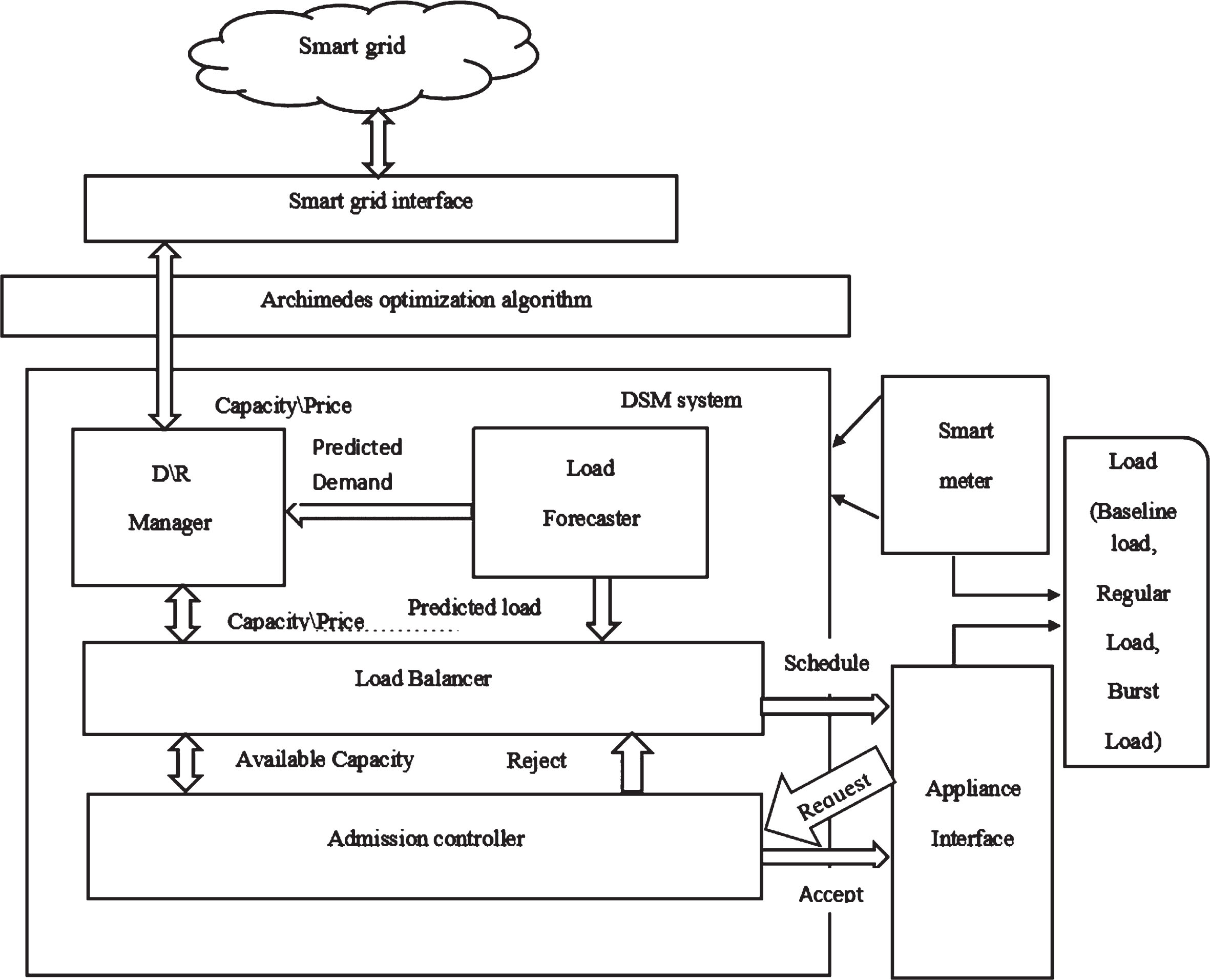
Proposed block diagram of Demand Side Management (DMS) with Archimedes Optimization Algorithm.

3.1 Baseline load

Baseline load is used to determine the capacity that is available for load balancing and admission control. should be taken into consideration. Even though the system does not regulate baseline load throughout operation, associated appliances can nevertheless communicate with the management system about their power usage and operational status via things like smart metres.

3.2 Burst load

It has to do with devices that must start and stop at specific times and have a fixed duration. Instances of these appliances are the laundry appliances, a dishwasher, and a dryer. In fact, The build-up of burst load is what causes the increase in peak load. Therefore, as it has a substantial impact on demand-side energy prices and power consumption efficiency, burst load control must be done carefully.

3.3 Regular load

It is the amount of energy used by appliances like water heaters and refrigerators that are continuously in operation over an extended period of time. However, because the connected appliances are susceptible to brief interruptions, admission control can be used to control how they operate. Regular loads are a particular instance of burst loads because they have certain features.

3.4 Admission control

Power access and appliance functioning are managed by the admission control. The AC will receive all requests and decide whether to allow or deny them based on the priority and admittance controller while always respecting the capacity limit.

3.5 Load Balancer

The LB will attempt to distribute the workload over a wider time horizon by receiving the rejected request that the AC is unable to handle. Based on number of time periods, energy cost, and capacity restriction, the LB will generate the best possible schedule. The LB notifies the appliances of the precise time to begin when the request has been scheduled. Events like new requests, changes to the capacity limit, and variations in the price of energy cause the timetable to be recalculated.

4 Modelling of demand side management

The scheduling, operation, and oversight of utility actions aimed at influencing user energy use in a way which will generate anticipated variations to the effectiveness’s load profile, or variations to the timing and size of a power load, is known as DSM, also known as demand-side optimization (DSO) [26]. There are a number of variables that affect how well a DSM approach performs. We shall analyse the more general characteristics that must be taken into account while creating any DSM technique in this part. One of the most important challenges in the DSM is the potential to be for a user or group of users dishonest and obtain additional benefits by straying from the actual energy consumption plan. A power management and controller scheme must be installed to enforce customers’ honesty and ensure that user communication does not compromise the ECS mechanism.

When considering the ECS, the scheduling time is equally crucial. The results will be better in terms of user comfort the faster the algorithm can run. Pre-emptive tasks, non-pre-emptive tasks, and the amount of time slots all factor into the execution time. On the basis of these hypotheses, the execution time can be shortened by up to 2 % while retaining access to the processing constraint mechanism. This technique shortens the search branching when the limited pinnacle currently extends the current best. The confined search is faster to execute and, hence, more stable as compared to non-constrained behaviour. The pre-emptive task’s search space size has a negative impact on the execution time. Constrained search can significantly increase computation speed by omitting the needless search space traversing.

Working process of Proposed DSM is shown in Fig. 2. Programs for demand response (DR), shifting the load, and efficiency of power are the fundamental components of DSM [27]. Residential users, for instance, can lower their energy usage by utilising efficient equipment [28]. The electric company may offer rewards for managing loads and participating in DR. Additionally, by informing people and raising awareness of the critical problem of peak hours, energy usage can be decreased. A DSM programme merely manages and transfers the energy as the use of low price per unit generating energy, the load can consume the same energy while paying less [29, 30]. It doesn’t always guarantee the restricted operation of loads. Flexible tariffs can contribute more to DSM if real-time data interchange with the smart grid is made possible.

Fig. 2

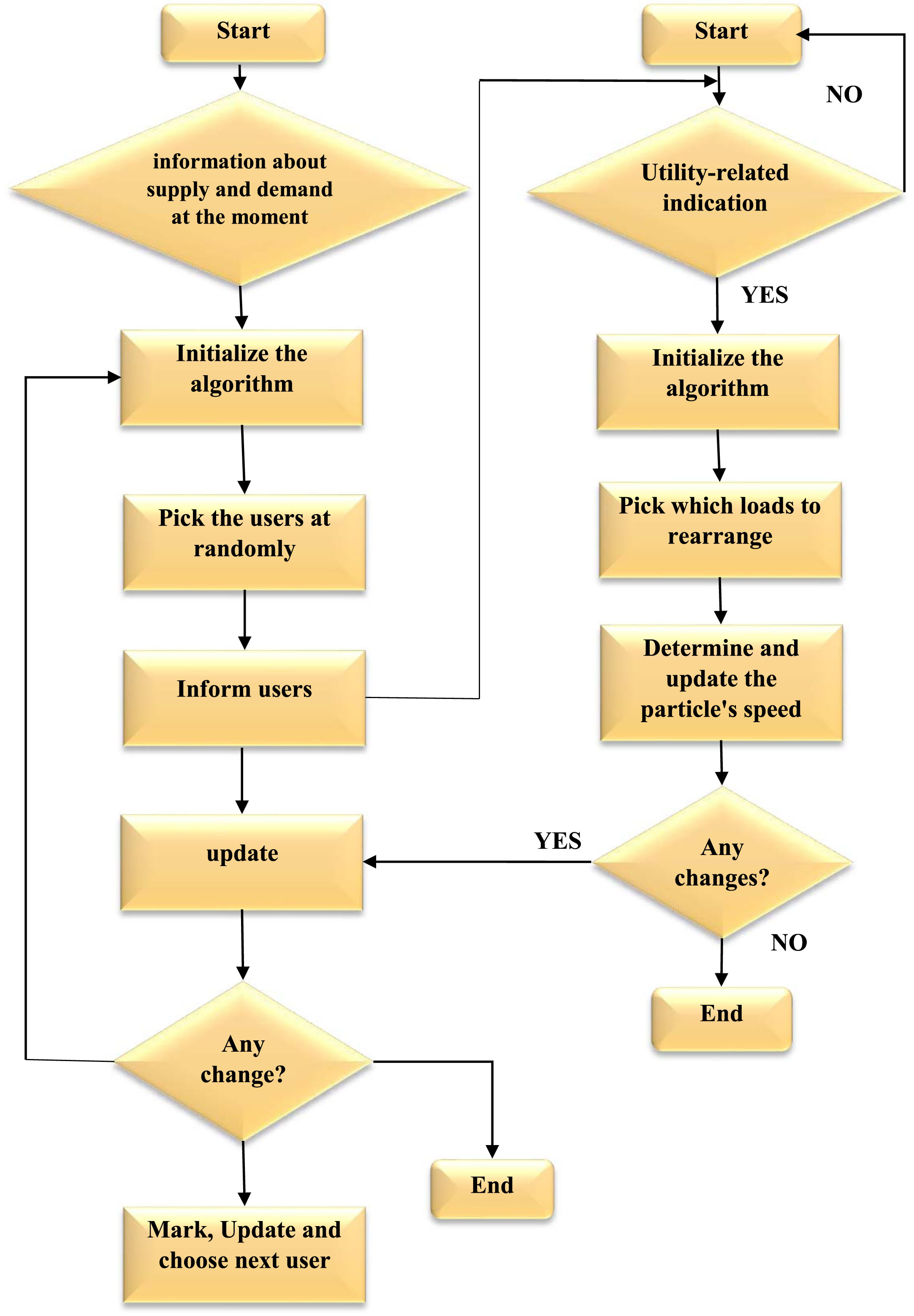
Working flow of proposed DSM.

Algorithm 1: Admission Control Algorithm

The signals coming from the request generator must be arranged in descending heuristic order

The factors (P_CL, P_Total, request sets A_i and B_j) should be initialized.

for all A_i ∈ A do

If a non pre-emptive appliance is running from an earlier time period,

Embrace A_i

Sum P_Ai to P_Total

Remove A_i from the demand set A.

end if

for all A_i ∈ A do

Request Ai is operating and pre-emptive if P_Total and P_AiP_CL.

Embrace A_i

Sum P_Ai to P_Total

Remove A_i from the request set A.

end if

A_i ∈ A do for all the remaining appliance demands

if P_Total + P_Ai ⩽ P_CL then

Embrace A_i

Sum P_Ai to P_Total

Remove A_i from the request set A.

Continue until there are no more requests waiting and the bandwidth is full.

end if

4.1 Mathematical modelling for load balancing

A DSM programme merely manages and transfers the load to consume the identical source of power but, with the decreased expenditures owing to the usage of low price per unit power production [31, 32]. It does not essentially ensure the reduced load performance. By Making real-time data available exchange with the SG, flexible tariffs can play a bigger role in DSM.

The assortment of utilizations can be symbolised by $A = (1, 2 \dots \dots . a)$ (1)

B displays the number of scheduling range time scales. $B = (1, 2, \dots \dots . b)$ (2)

A specific device’s rated power, P_Ai, and rated energy consumption, Energy_Ai, can be used to specify the amount of time frames that can be allotted for that item. Since power is well-defined as “ speed at which energy is converted,” the entire time required for an item to finish its function may be statistically expressed as, which we must state. $T_{Ai} = \frac{{Energy}_{Ai}}{P_{Ai}}$ (3)

4.2 Problem optimization

In our suggested approach, we assume that a user’s scheduling horizon is one day, or 24 hours. At the beginning of the day, the user enters all the appliances that must be used on that particular day. Through the user interfaces, the user can also specify how the appliances should be configured. A single day’s scheduling limit can be shown as, $t_{s} \in T = (1, 2, \dots . ., T) .$ (4) where T = 24 Delayable Appliances (DAs) and Non-Delayable Appliances make up the set of home appliances for a single user (NDAs). Timed appliances (TAs) were listed on the Table 2.

Table 2

List of timed appliances (TAs)

S.No	Appliance	Power (kwh)	T _L	T _U	l_dai (hr)	WTA _Max
1	Washing Machine	0.78	9	17	1.5	6.5
2	Dish Washer	3.6	8	13	1.6	3
3	Clothes Dryer	4.4	7	19	2.1	11
4	PHEV	3.6	19	25	3.2	4

$Total Household Appliances = ({DA}_{s} + {NDA}_{s})$ (5)

Hence the set of DAs can be written as, where TA stands for Timed Appliances, and RA stands for Regular Appliances. Regular appliances (RAs) were listed on the Table 3.

Table 3

Regular appliances list (RAs)

S.No	Appliances	power (kWh)	T _L	T _U	Priority
1	Conditioning unit	1.45	6	24	1
2	Refrigerator	0.735	6	24	2
3	Water Heater	4.55	6	24	3
4	Space Heater	1.6	6	24	4

${DA}_{s} = ({TA}_{s} + {RA}_{s})$ (6) $d_{a} \in {DA}_{S} = ({da}_{1}, {da}_{2} \dots \dots \dots, {da}_{n})$ (7)

The total amount of power needed by each DA to finish its function is $P_{da} = (P_{da 1}, P_{da 2}, \dots \dots \dots, P_{dan})$ (8)

Additionally, each DA’s hourly power consumption is provided as follows: $x_{da} = (x_{da 1}, x_{da 2}, \dots \dots ., x_{dan})$ (9)

The lower threshold of time (T_L) and the upper bound of time (T_U) specified for each appliance, respectively, will now be described as a adjustable direction of initial period settings of DA_s inside T_LandT_U. $t_{a} = (t_{a 1}, t_{a 2}, \dots \dots . ., t_{an})$ (10)

and the collection of restrictions might be described as $t_{s} \in [T_{L}, LST]$ $T_{L} ⩽ t_{s} ⩽ LST$

where LST is the newest starting period for TA_s, from that T_A process requirement activate.

4.3 Billing mechanism

We take into account a dynamic billing system for the application of our model. Load synchronisation, or the phenomena of significant load building right just after peak hour price ends, is the most important problem with RTP. We have developed two criteria for ensuring power capacity limits in order to avoid the load synchronisation issue and progress the constancy of an electrical energy sector. The IBR is the first, as seen below. $C_{t_{s}} x_{t_{s}} = {\begin{matrix} C_{t_{s}}^{1}, if 0 ⩽ x_{t_{s}} ⩽ x_{th} \\ C_{t_{s}}^{2}, if x_{t_{s}} > x_{th} \end{matrix}$ (11)

Where x_{t
_s} is the total volume of power used at time span t_s and x_th is the threshold amount of energy consumption. Additionally, $C_{t_{s}}^{1} and C_{t_{s}}^{2}$ are 2 distinct value prices, and they are constantly equal. The overall power consumption cap for a specific billing period makes up the second criterion. Residential consumers pay 7.53 c/kWh for first 1,360 kwh they consume over a typical two-month billing cycle, according to this model. Customers will charge 11.27 cents a kwh after exceeding the maximum allowed power consumption.

4.4 Minimizing energy costs

The formula for cost minimization can be expressed as, $\sum_{da \in DA} X_{da}^{t_{s}} ⩽ P_{CL}$ ${WTA}_{da} ⩽ {WTA}_{da (Max)}$ $t_{s} \in [T_{L}, LST]$

The P_CL is the highest volume of power which will be used by each user during a certain billing cycle, as determined by the power distribution company. The user-specified maximum interruption for each utilization is represented by WTA_da-Max.

4.5 PAR reduction

The total amount of energy used by a single appliance during various time periods can be expressed as, $X_{Load (da)} = \sum_{t_{s} = 1}^{T} x_{da}^{t_{s}}$ (12)

Nowadays, the daily power usage of a single person can be expressed as, $X_{Load} = \sum_{t_{s} = 1}^{T} \sum_{da \in DA} x_{da}^{t_{s}}$ (13)

A single user’s maximum and average power usage at a given period can be used to determine the PAR, which can be expressed as, $PAR = \frac{max (X_{Load})}{avg (X_{Load})}$ (14)

the PAR becomes more complex for a huge number of participants. $minimize PAR = \frac{\sum_{n = 1}^{N} max (X_{Load})}{\frac{1}{T} \sum_{n = 1}^{N} (X_{Load})}$ (15)

5 Proposed archimedes optimization (AO) algorithm

To determine the ideal value of power consumption within the scheduled time period, AO-based optimization is used. The goal of AO is to imitate the forecasting of utilizations in a way that is necessary for evolution. AO Algorithm-based optimal DSM will ultimately improve the smart grid’s performance while also reducing the price of electricity usage. The population-based algorithm known as AO. Individuals in the objects serve as the absorbed substances in the suggested approach. The search procedure for AO Algorithm begins with an initial population of objects (candidates), just like other population-based metaheuristic algorithms. solutions) with erratic accelerations, densities, and volumes. Each object is initialised at this point with a random spot in the fluid. AO Algorithm performs iterations until the termination circumstance is met after assessing the basic population’s efficiency. The density and volume of each item are updated by AO Algorithm after every iteration. Depending on whether an object collides with any other nearby objects, its acceleration is changed. The new position of a population is calculated by the revised dimensions, intensity, and speed. The exact mathematical representation of the AO Algorithm stages is represented below.

Algorithm 2: Archimedes Optimization (AO) Algorithm

Procedure

AOA (population size N, maximum iterations t_max, C₁, C₂, C₃ and C₄)

Create a population of objects with random placements, velocities, and dimensions using the appropriate methods.

Choose the beginning population with the highest fitness value after evaluating the others.

Set iteration counter t=1

Whilet ⩽ t_maxdo

for each object ido

Data updates for each object’s dimension and intensity

if energy consumption per hour (i)>Maximum Limit

Maximum Energy Consumption = Total consumption energy-Predefine energy

Check if Maximum Energy Consumption < Energy of shiftable load

Shift the shiftable loads

else

i = i+1;

Update transfer and intensity decreasing factors TF and d correspondingly.

if TF⩽ 0.5 then

Increase and normalise acceleration data

Updata position

else

Updata acceleration and normalize acceleration

Updata direction flag F

Updata position

end if

end for

Choose the object with the highest fitness value after evaluating each item.

Set t = t + 1

end While

Set all objects’ positions to zero using (16): $O_{i} = {lb}_{i} + rand \times ({ub}_{i} - {lb}_{i}); i = 1, 2, \dots . . N$ (16)

For iteration t + 1, the density and volume of object i are changed with (17) ${den}_{i}^{i + 1} = {den}_{i}^{t} \times ({den}_{best} - {den}_{i}^{t})$ (17) ${vol}_{i}^{i + 1} = {vol}_{i}^{t} \times rand ({vol}_{best} - {vol}_{i}^{t})$ (18)

When A uniformly distributed random number is called a rand, volt_best and den_best are the density and volume corresponding to the best population so far discovered.

This is accomplished in AO Algorithm with the aid of the transfer operator T F, specified in (19), which changes search from exploration to exploitation: $TF = exp (\frac{t - t_{Max}}{T_{Max}})$ (19)

Similar to how it helps AOA with local to global search, density reducing factor d. It gets smaller over time utilising (20): $d^{t + 1} = exp (\frac{t_{Max} - t}{t_{Max}}) - (\frac{t}{t_{Max}})$ (20)

When an item collides with another if T F < 0.5, For iteration t + 1, alter the object’s acceleration using (21): ${acc}_{i}^{t + 1} = \frac{{den}_{mr} + {vol}_{mr} \times {acc}_{mr}}{{den}_{i}^{t + 1} \times {vol}_{i}^{t + 1}}$ (21)

Update the population’s acceleration for iteration t + 1 by (22) if T F > 0.5, which indicates that there is no object collision: ${acc}_{i}^{t + 1} = \frac{{den}_{best} + {vol}_{best} \times {acc}_{best}}{{den}_{i}^{t + 1} \times {vol}_{i}^{t + 1}}$ (22)

To determine the percentage of change, normalise acceleration using (23):

${acc}_{i - norm}^{t + 1} = u \times \frac{{acc}_{i}^{t + 1} - min (acc)}{max (acc) - min (acc)} + 1$ (23) where u and l, which are fixed to 0.9 and 0.1, correspondingly, are the normalisation ranges. The percentage of steps that each agent will alter is determined by the ${acc}_{i}^{t + 1}$ .

$\begin{matrix} x_{i}^{t + 1} = x_{i}^{t} + C_{1} \times rand \\ \times {acc}_{i - norm}^{t + 1} \times d \times (x_{rand} - x_{i}^{t}) \end{matrix}$ (24) where C1 equals a constant of 2. In the absence of this, if T F > 0.5, the items upgrade their positions using (25).

$\begin{matrix} x_{i}^{t + 1} = x_{best}^{t} + F \times C_{2} \times rand \times {acc}_{i - norm}^{t + 1} \\ \times d \times (T \times x_{best} - x_{i}^{t}) \end{matrix}$ (25) where a constant called C2 = 6. T is defined by T = C3 T F and rises over time while being proportionate to the transfer agent directly. T primarily deducts a fixed percentage first from best possible position and grows with time in the range [C3 0.3, 1]. Starting with a low percentage results in a significant gap amongst the optimal and the present position, which causes the random walk’s step size to be high. This percentage gradually rises as the search goes for reducing the distance is necessary between the ideal position and the present position.

6 Results and discussion

This section discusses the simulation findings that were achieved using MATLAB/Simulink. The results of the simulations demonstrate how effectively the suggested DSM method manages a great amount of controllable loads. To decrease costs and the PAR, the suggested algorithm adjusts the load. In terms of lowering peak load demand, lowering power consumption costs, and raising consumer comfort levels, the simulation findings of our suggested power consumption scheduling arrangement are highly effective. With a different design strategy, our suggested technique moves the use of appliances used in the home at peak and off-peak times, hence reducing peak demand. The recognized issue with the reduction of peak load for SG stability and power rate savings has been mentioned in our plan [33, 34]. The appliances are controlled by optimal scheduling so that high loads are operated during off-peak times. Our scheduling method addresses this issue by introducing a threshold for the energy use when off-peak and peak hours. The cycle of an appliance’s operation is switched to off-peak hours if its assessments are larger than the criterion price.

Our plan has made reference to the issue of reducing energy loss from standby appliances in homes. An appliance’s standby power is the amount of energy used when it is not in use or when it is turned off. Ten percent of electricity is used by standby equipment. It has been suggested that standby strategies contribute to power waste, hence it was important to address this waste while scheduling household appliances to enable DSM. Furthermore, by limiting an appliance’s delay factor, our suggested scheduling approach raises the consumer’s degree of comfort. The cycle is preserved and the appliance is turned ON right away if the cycle is moved to off-peak hours and the delay exceeds the limit.

Here, three end users and 10 electrical appliances are taken into account to reduce costs. However, the duration of usage for each appliance varies depending on the user’s requirements. Each appliance’s KVA rating is regarded as being the same. However, shiftable loads, whose times of usage can be adjusted to coincide with periods of lower grid load, play a major role. Table 4 lists the input information for household load appliances.

Table 4
List of non-delayable appliances (NDAs)

S.No Appliances power (kWh)

1 Lighting 0.06

2 Entertainment 0.15

3 Fans 0.75

4 Cloths Iron 1.5

5 Microwave Oven 1.18

6 Toaster 0.05

7 Laptop Charger 0.05

S.No	Appliances	power (kWh)
1	Lighting	0.06
2	Entertainment	0.15
3	Fans	0.75
4	Cloths Iron	1.5
5	Microwave Oven	1.18
6	Toaster	0.05
7	Laptop Charger	0.05

In Fig. 3, the electricity use of consumers during a 24-hour period is shown for both scenarios, with and without scheduling. The load climbs to 40kwh during peak hours. Residential load input was represented in Table 5. When we arrange the appliances in accordance with our suggested plan, the load is distributed fairly throughout the day. consumption of energy drops to 20%.

Fig. 3

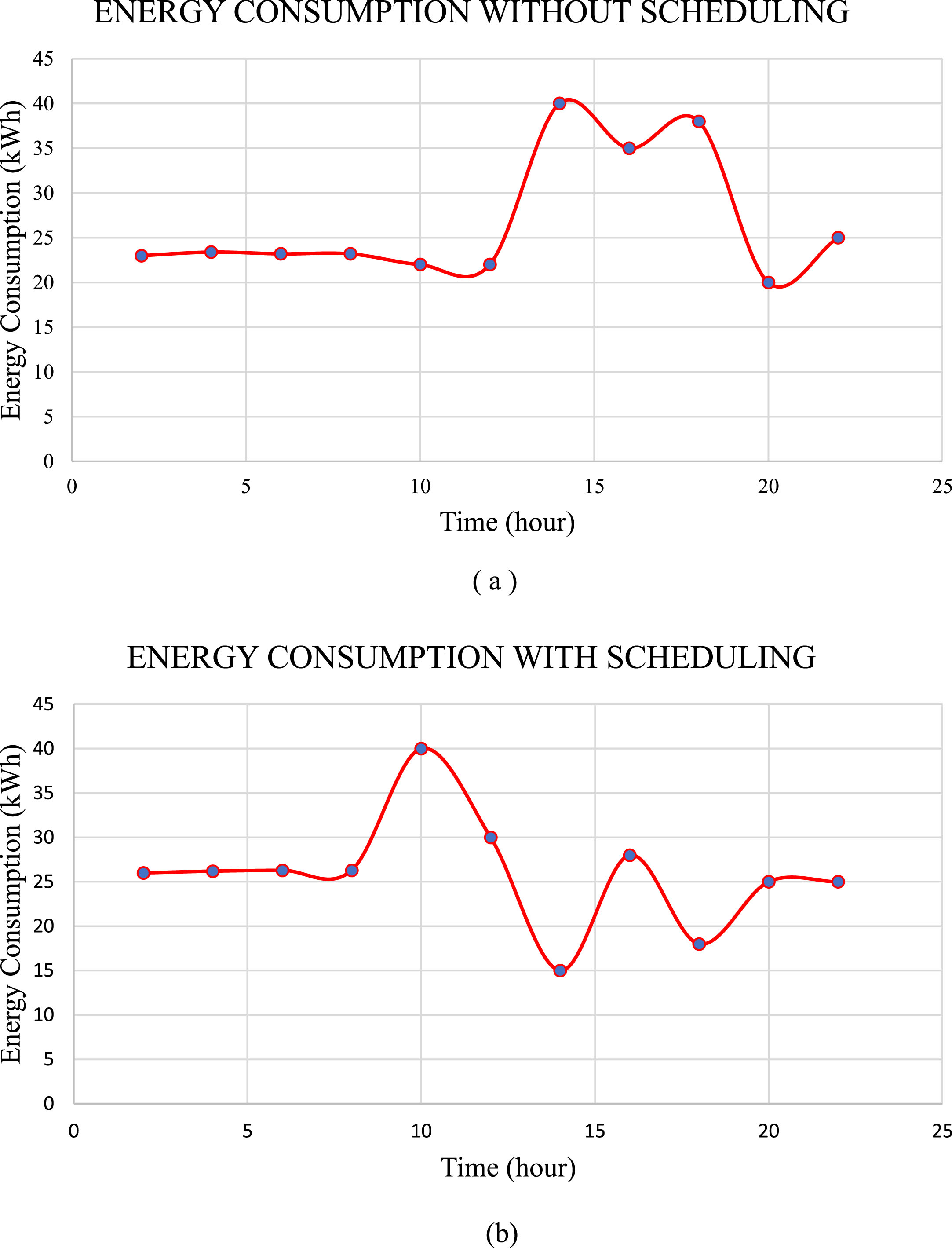
Energy use with and without scheduling.

Table 5

Residential load input

S.No	Name of Appliances	Type of Appliance	Power Consumption (KWH)
1	Iron	Shiftable Load	0.16
2	Toaster	Shiftable Load	2.3
3	TV	shiftable Load	1.2
4	Washing Machine	shiftable Load	3.2
5	Fan	shiftable Load	0.33
6	Fridge	Non-shiftable Load	2.5
7	Air Conditioner	Non-shiftable Load	3.4
8	Geyser	Non-shiftable Load	5.6
9	Aquarium Pump	Non-shiftable Load	0.21
10	Water	Non-shiftable Load	0.16

Figure 4 shows the AO Based energy use with and without scheduling during a 24-hour period. The load climbs to 30 kwh during peak hours. When we arrange the appliances in accordance with our suggested plan, the load is distributed fairly throughout the day. consumption of energy drops to 15%. Figure 5 depicts the peak hour % load for each user with and without scheduling for home appliances. According to the simulation results, the % load is large when energy usage units are not incorporated in smart metres (both without and with schedule of home appliances). Without scheduling, the energy consumption unit more effectively schedules the power consumption, bringing down the peak load to 20%. Energy consumption unit plans the energy usage more effectively, bringing down the peak load to 15%.

Fig. 4

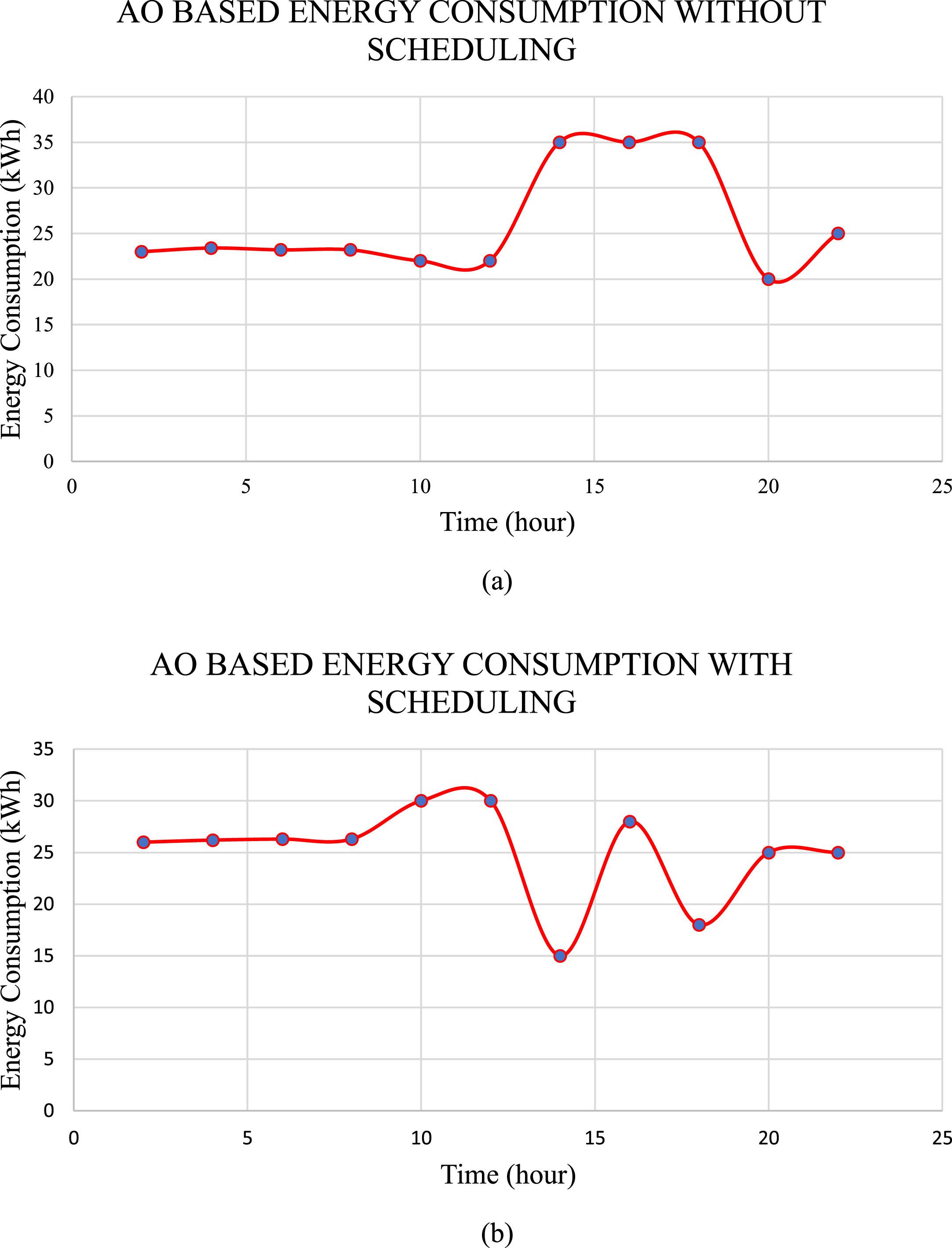
AO Based energy use with and without scheduling.

Fig. 5

Percentage of users during peak hours.

By using our effective power consumption scheduling technique for control of load, we also reduce the financial cost. Figure 5 represents the percentage load of users during peak times. When all subscribers and users of smart metres equipped with ECC units use the energy efficiently, the cost of energy is reduced by 21%. Each user’s monthly expense is reduced by arranging energy use. Figure 6 displays the monthly bill reduction for each user, demonstrating how scheduling appliances can reduce each customer’s utility payments. Comparison of various DSM techniques with different optimization algorithm were represented in Table 6.

Fig. 6

Estimated expenditure charges for every user, both with and without scheduling.

Table 6

Comparison of various DSM techniques with different optimization algorithm [35 –41]

S.No	Author’s Name and Year	Methodology	Outcome
1	Sergio Nicolas Bragagnolo et al. year 2021	Comparison of Demand Side Management’s Technical and Economic Criteria Using a Multi-Level Optimization Model	It increases retailer profit by improving the demand profile. But when the provider strives to maximise profit, certain users benefit at the expense of others, leading to the conclusion that the technological method is superior than the economical one, which has a 90% efficiency.
2	SajjadAli et al. year: 2022	Day-ahead scheduling difficulty can be overcome using multi-objective energy optimization for DMS in the smart grid.	The day ahead scheduling multi-objective problem is resolved using the MOWDO method, according to simulation results, in order to lower operational costs, reduce pollution, and satisfy end users.
3	JavadEbrahimi et al. year: 2022	A two-stage framework combining reliable optimization algorithms for demand-side control and energy savings of different buildings in several smart grids	In comparison to IGWO, it lowers the generation costs of commercial, residential and industrial microgrids by more than 3.6, 2.1, and 3.8 percent. In many instances, the CPLEX solver delivers results that are superior to those of the IGWO.
4	PuttamadappaC et al. year: 2019	Utilizing the glow-worm swarm optimization technique, DMS of minor loads in a smart grid	It lowers energy costs by 11.2 percent, enabling decision-makers to balance stability by taking the appropriate demand-side activities.
5	Haider TarishHaider et al. year: 2021	An innovative method for smart grids’ multi-objective cost-peak demand response for residential areas	For the time of usage and adaptive consumption level pricing schemes, it reduces end-user energy costs by more than 80% and 76%, respectively. For the baseline operation, the end-user peak load has been decreased by 55%.
6	AhmedShaban et al. year: 2021	A cuckoo load scheduling optimization technique for demand side management	It manages to save anywhere between 57 and 80 percent on energy costs.
7	Proposed	Demand Side Management in a Smart Grid Environment Using a Novel Archimedes Optimization Algorithm	It lowers the PAR, the overall energy cost, and the daily electricity costs for each user. According to the results of the simulation, the DSM model reduces a single user’s PAR by 18.17 percent and minimises energy costs by 89.49 percent. When there are numerous users, the reduction in PAR and total energy costs are 46.85% and 53.24%, respectively.

The graph of the residential load without and with scheduling is shown in Fig. 7. The Archimedes Optimization (AO) technique is employed for controllable load scheduling. The loads taken into consideration have various average power values and limited on-time intervals. The proposed algorithm’s implementation demonstrates that all loads will be planned. Additionally, it displays the decline in price and PAR.

Fig. 7

Without and with scheduling graph for residential load.

7 Conclusion

In this paper, the Archimedes Optimization (AO) Method is used to propose the DSM algorithm for residential loads. In this regard, a load scheduling problem is taken into account for the aforementioned users, including shiftable and non-shiftable devices, and is resolved using the Archimedes Optimization (AO) Algorithm. The outcome of a MATLAB simulation demonstrates that each user efficiently uses the energy and minimises the overall cost per day. Additionally, the entire SG benefits from this suggested technique, especially at the level of the distribution network. The capacity and reliability of the distribution network are boosted by a decrease in peak load demand. Finally, the findings demonstrate that the suggested algorithm successfully lowers the user’s PAR ratio, which in turn lowers the cost of electricity use. The outcomes demonstrate that the suggested DSM model with AO Algorithm lowers PAR, total energy cost, and daily electricity rates for each user. According to the results of the simulation, the DSM model reduces a single user’s PAR by 18.17 percent and minimises energy costs by 89.49 percent. When there are numerous users, the reduction in PAR and total energy costs are 46.85% and 53.24%, respectively. This model might be revised in the future to account for energy production at the user side, such as solar, wind, and fuel cells.

References

Bragagnolo

Sergio Nicolas

, Vaschetti

Jorge Carlos

and Magnago

Fernando

, On the scalability of supply cost for demand management in the smart grid, IEEE Latin America Transactions 20(4) (2022), 643–650.

Saleem

M. Usman

, Usman

M. Rehan

, Usman

M. Arslan

and Politis

Christos

, Design, Deployment and Performance Evaluation of an IoT Based Smart Energy Management System for Demand Side Management in Smart Grid, IEEE Access 10 (2022).

Bragagnolo

Sergio Nicolas

, Vaschetti

Jorge Carlos

and Magnago

Fernando

, A Technical and Economic Criteria Comon on Demand Side Management with Multi-Level Optimization Model, IEEE Latin America Transactions 19(9) (2021), 1494–1501 paris.

Corbett

Jacqueline

, Wardle

Katherine

and Chen

Chialin

, Toward a sustainable modern electricity grid: The effects of smart metering and program investments on demand-side management performance in the US electricity sector 2009–2012, IEEE Transactions on Engineering Management 65(2) (2018).

Mansiri

Kongrit

, Sukchai

Sukruedee

and Sirisamphanwong

Chatchai

, Fuzzy Control Algorithm for Battery Storage and Demand Side Power Management for Economic Operation of the Smart Grid System at Naresuan University, Thailand, IEEE Access 6 (2018).

Nawaz

Abdullah

, Hafeez

Ghulam

, Khan

Imran

, Jan

Khadim Ullah

, Li

Hui

, Khan

Sheraz Ali

and Wadud

Zahid

, An Intelligent Integrated Approach for Efficient Demand Side Management With Forecaster and Advanced Metering Infrastructure Frameworks in Smart Grid, IEEE Access 8 (2020).

Chandra

Rohit

, Banerjee

Soumen

, Radhakrishnan

Krishnanand Kaippilly

and Panda

Sanjib Kumar

, Transactive Energy Market Framework for Decentralized Coordination of Demand Side Management Within a Cluster of Buildings, IEEE Transactions on Industry Applications 57(4) (2021), 3385–3395.

Chen

Wenbo

, Zhou

Anni

, Zhou

Pan

, Gao

Liang

, Ji

Shouling

and Wu

Dapeng

, A Privacy-Preserving Online Learning Approach for Incentive-Based Demand Response in Smart Grid, IEEE Systems Journal 13(4) (2019).

Tan

, Xiao

Yuanzhang

and Song

Linqi

, Integrating Future Smart Home Operation Platform With Demand Side Management via Deep Reinforcement Learning, IEEE Transactions on Green Communications and Networking 5(2) (2021), 921–933.

10.

Yang

Hongming

, Zhang

Jun

, Qiu

Jing

, Zhang

Sanhua

, Lai

Mingyong

and Dong

Zhao Yang

, A Practical Pricing Approach to Smart Grid Demand Response Based on Load Classification, IEEE Transactions on Smart Grid 9(1) (2018), 179–190.

11.

Kong

Peng-Yong

, Radio Resource Allocation Scheme for Reliable Demand Response Management Using D2D Communications in Smart Grid, IEEE Transactions on Smart Grid 11(3) (2020).

12.

Samadi

Pedram

, Mohsenian-Rad

Hamed

, Schober

Robert Wong

and Vincent

W.S.

, Advanced Demand Side Management for the Future Smart Grid Using Mechanism Design, IEEE Transactions on Smart Grid 3(3) (2012), 1170–1180.

13.

Safdarian

Amir

, Lehtonen

Matti

, Fotuhi-Firuzabad

Mahmud

and Billinton

Roy

, Customer Interruption Cost in Smart Grids, IEEE Transactions on Power Systems 29(2) (2014).

14.

Nawaz

Abdullah

, Hafeez

Ghulam

, Khan

Imran

, Jan

Khadim Ullah

, Li

Hui

, Khan

Shiraz Ali

and Wadud

Zahid

, An Intelligent Integrated Approach for Efficient Demand Side Management with Forecaster and Advanced Metering Infrastructure Frameworks in Smart Grid, IEEE Access 1(1) (2020).

15.

Costanzo

Giuseppe Tommaso

, Zhu

Guchuan

, Anjos

Miguel F.

and Savard

Gilles

, A System Architecture for Autonomous Demand Side Load Management in Smart Buildings, IEEE Transactions on Smart Grid 3(4) (2012), 2157–2165.

16.

Ahmad

Sadiq

, Ahmad

Ayaz

, Shoukat

Abdullah

, Behram

Belawal

, Khan

Saad Salman

and Yaqub

Raziq

, Consumer Energy Management in Residential Distribution Power System Considering Consumer’s Privacy, (2021).

17.

Wang

Kun

, Li

Huining

, Maharjan

Sabita

, Zhangand

Yan

Guo

Song

, Energy Scheduling for Demand Side Management in the Smart Grid, IEEE Transactions on Green Communications and Networking 1(1) (2018)–Green.

18.

Liu

, Yuen

, Huang

, Ul Hassan

, Wang

and Xie

, Peak-to-Average Ratio Constrained Demand-Side Management With Consumer’s Preference in Residential Smart Grid, IEEE Journal of Selected Topics in Signal Processing 8(6) (2014), 1084–1097.

19.

Balli

Muhammed

, Uludag

Suleyman

, Selcuk

Ali

and Tavli

Bulent

, Distributed Multi-Unit Privacy Assured Bidding (PAB) for Smart Grid Demand Response Programs, IEEE Transactions on Smart Grid 1(1) (2017).

20.

Feng

, Qian

and Hu

Rose

, A Real-Time Information Based Demand-Side Management System in Smart Grid, IEEE Transactions on Parallel and Distributed Systems 1(1) (2015).

21.

W.-T.

, Yuen

, Hassan

N.U.

, Tushar

, Wen

C.-K.

, Wood

K.L.

… and Liu

, Demand Response Management for Residential Smart Grid: From Theory to Practice, IEEE Access 3 (2015), 2431–2440.

22.

Wang

Kun

, Li

Huining

, Maharjan

Sabita

, Zhang

Yan

and Guo

Song

, Energy Scheduling for Demand Side Management in the Smart Grid, IEEE Transactions on Green Communications and Networking 2(2) (2018)–Green.

23.

Balli

Muhammed Fatih

, Uludag

Suleyman

, Selcuk

Ali Aydin

and Tavli

Bulent

, Distributed Multi-Unit Privacy Assured Bidding (PAB) for Smart Grid Demand Response Programs, IEEE Transactions on Smart Grid 9(5) (2018).

24.

Stephens

Edward R.

, Smith

David B.

and Mahanti

Anirban

, Game Theoretic Model Predictive Control for Distributed Energy Demand-Side Management, IEEE Transactions on Smart Grid 6(3) (2015), 1394–1402.

25.

Kaewpuang

, Niyato

and Wang

Ping

, Decomposition of Stochastic Power Management for Wireless Base Station in Smart Grid, 1(2) (2012), 97–100.

26.

Cecati

, Citro

and Siano

, Combined Operations of Renewable Energy Systems and Responsive Demand in a Smart Grid, 2(4) (2011), 468–476.

27.

Mortaji

Hamed

, Ow

Siew Hock

, Moghavvemi

Mahmoud

and Almurib

Haider A.F.

, Load Shedding and Smart-Direct Load Control Using Internet of Things in Smart Grid Demand Response Management, IEEE Transactions on Industry Applications 1(1) (2017).

28.

Song

Linqi

, Xiao

Yuanzhang

and van der Schaar

Mihaela

, Demand Side Management in Smart Grids Using a Repeated Game Framework, IEEE Journal on Selected Areas in Communications 32(7) (2014), 1412–1424.

29.

Dan

, SUN

Hongjian

, Chiu

Wei-Yu

, and Poor

, Multi objective Optimization for Demand Side Management in Smart Grid, IEEE Transactions on Industrial Informatics (2017)–Vincent.

30.

Adika

Christopher O.

and Wang

Lingfeng

, Demand-Side Bidding Strategy for Residential Energy Management in a Smart Grid Environment, IEEE Transactions on Smart Grid 5(4) (2014), 1724–1733.

31.

Chen

Wenbo

, Zhou

Anni

, Zhou

Pan

, Gao

Liang

, Ji

Shouling

and Wu

Dapeng

, A Privacy-Preserving Online Learning Approach for Incentive-Based Demand Response in Smart Grid, IEEE Systems Journal (2019), 1–11.

32.

Tan

, Xiao

Yuanzhang

and Song

Linqi

, Integrating Future Smart Home Operation Platform With Demand Side Management via Deep Reinforcement Learning, IEEE Transactions on Green Communications and Networking 5(4) (2021).

33.

Saleem

M. Usman

, Usman

M. Rehan

and Shakir

Mustafa

, Design, Implementation, and Deployment of an IoT Based Smart Energy Management System, IEEE Access 5(8) (2021).

34.

Palensky

and Dietrich

, Demand Side Management: Demand Response, Intelligent Energy Systems, and Smart Loads 7(3) (2011), 0–388.

35.

Qian

, Feng

Zhiyong

, Li

Wei

, Gulliver

T. Aaron

and Zhang

Ping

, Joint Spatial and Temporal Spectrum Sharing for Demand Response Management in Cognitive Radio Enabled Smart Grid, IEEE Transactions on Smart Grid 5(4) (2014), 1993–2001.

36.

Luo

Fengji

, Kong

Weicong

, Ranzi

Gianluca

and Yang

Zhao Dong

, Optimal Home Energy Management System with Demand Charge Tariff and Appliance Operational Dependencies, IEEE Transactions on Smart Grid 7(8) (2019).

37.

Kong

Peng-Yong

, Radio Resource Allocation Scheme for Reliable Demand Response Management using D2D Communications in Smart Grid, IEEE Transactions on Smart Grid 6(7) (2019).

38.

Iqbal

M.M.

, Zia

M.F.

, Beddiar

and Benbouzid

, Optimal Scheduling of Grid Transactive Home Demand Responsive Appliances Using Polar Bear Optimization Algorithm, IEEE Access 8 (2020), 222285–222296.

39.

Zafar

Usman

, Bayhan

Sertac

and Sanfilippo

Antonio

, Home Energy Management System Concepts, Configurations, and Technologies for the Smart Grid, IEEE Access 34(3) (2020).

40.

Tan

Zhao

, Yang

Peng

and Nehorai

Arye

, An Optimal and Distributed Demand Response Strategy With Electric Vehicles in the Smart Grid, IEEE Transactions on Smart Grid 5(2) (2014), 861–869.

41.

Zhang

, Hu

, Dai

, Dang

, Yao

and Zhou

, Unit Commitment Model in Smart Grid Environment Considering Carbon Emissions Trading, IEEE Transactions on Smart Grid 7(1) (2016), 420–427.

Demand side management using a novel archimedes optimization algorithm in a smart grid environment

Abstract

Keywords

1 Introduction

3 Proposed methodology

3.2 Burst load

3.3 Regular load

3.4 Admission control

3.5 Load Balancer

4 Modelling of demand side management

4.5 PAR reduction

Table 4 List of non-delayable appliances (NDAs) S.No Appliances power (kWh) 1 Lighting 0.06 2 Entertainment 0.15 3 Fans 0.75 4 Cloths Iron 1.5 5 Microwave Oven 1.18 6 Toaster 0.05 7 Laptop Charger 0.05

References

Table 4
List of non-delayable appliances (NDAs)

S.No Appliances power (kWh)

1 Lighting 0.06

2 Entertainment 0.15

3 Fans 0.75

4 Cloths Iron 1.5

5 Microwave Oven 1.18

6 Toaster 0.05

7 Laptop Charger 0.05