A cubic fuzzy graph is a fuzzy graph that simultaneously supports fuzzy membership and interval-valued fuzzy membership. This simultaneity leads to a better flexibility in modeling problems regarding uncertain variables. The cubic fuzzy graph structure, as a combination of cubic fuzzy graphs and graph structures, shows better capabilities in solving complex problems, especially where there are multiple relationships. Since many problems are a combination of different relationships, as well, applying some operations on them creates new problems; therefore, in this article, some of the most important product operations on cubic fuzzy graph structure have been investigated and some of their properties have been described. Studies have shown that the product of two strong cubic fuzzy graph structures is not always strong and sometimes special conditions are needed to be met. By calculating the vertex degree in each of the products, a clear image of the comparison between the vertex degrees in the products has been obtained. Also, the relationships between the products have been examined and the investigations have shown that the combination of some product operations with each other leads to other products. At the end, the cubic fuzzy graph structure application in the diagnosis of brain lesions is presented.
Graphs are the mathematical language of systems whose components have internal connections and are comparable to nodes and edges in a graph theory. The combination of these relationships with each other causes the complexity of modeling in some issues. When there is no certainty in the modeling of objects and the relationship between them, it is necessary to use models based on fuzzy environment. The idea presented by Zadeh [1] in the description of Fuzzy Set (FS) in 1965 became the basis for one of the most important concepts in the field of fuzzy and uncertain topics. This concept quickly found wide applications in computer science, information science, system science, management science, theoretical mathematics and other fields of science. A decade after the introduction of FS, Zadeh presented an interval-valued fuzzy set (IVFS) as a branch of FS in which an interval between 0 and 1 was used as the membership value instead of a fuzzy number. These two concepts gave rise to different types of graphs called fuzzy graphs, which were first introduced by Kaufman [2] in 1973. Later, fuzzy graph theory was developed as a generalization of graph theory by Rosenfeld [3] in 1975. He explained some concepts including tree, cut vertex, cycle, bridge, and end vertex in fuzzy graphs. The researchers studied different types of fuzzy graphs. Talebi [4] had a study on Kayley fuzzy graph. Borzooei et al. [5, 6] had many studies on vague graphs. Atanassov [7] introduced the concept of intuitionistic fuzzy set (IFS) as a generalization of FS. Akram and Dudek [8] gave the idea of an interval-valued fuzzy graph (IVFG) in 2011. Talebi et al. [9, 10] introduced some new concepts of interval-valued intuitionistic fuzzy graph (IVIFG). Kosari et al. [11–13] studied new results in vague graph and vague graph structures. Rao et al. [14, 15] defined dominating set and equitable dominating set in vague graphs. Certain properties of domination in product vague graphs were examined by shi et al. [16]. Shao et al. [17] introduced IFGs concepts which were used in the water supplier systems. Rashmanlou et al. [18] explained Ring sum in products with intuitionistic fuzzy graphs.
Graph structures were presented by Sampathkumar [19] in 2006 as a generalization of signed graphs and graphs with labeled or colored edges. Fuzzy graph structure (FGS) is more important than graph structure because uncertainty and ambiguity in many real-world phenomena often occur as two or more separate relationships. Dinesh [20] introduced the notion of an FGS and discussed some related properties. Ramakrishnan and Dinesh [21] generalized this concept in studies. Akram [22] presented new results on m-polar FGSs. Akram and Akmal [23–25] investigated the concepts of bipolar FGSs and intuitionistic FGSs. Akram et al. [26–30] defined new concepts of operations in FGSs. Kou et al. [31] studied vague graph structure. Continuing his studies in 2020, Denish [32] presented the concept of fuzzy incidence graph structure. Akram and Sitara [33] introduced decision-making with q-rung orthopair FGSs. Sitara and Zafar [34] studied the application of q-rung picture FGSs in airline services
Fuzzy graphs were previously limited to one or more degrees of fuzzy membership or interval-valued fuzzy membership. Jun et al. [35] introduced the idea of a cubic fuzzy set (CFS) in the form of a combination of FS and IVFS, which serves as a more general tool for modeling uncertainty and ambiguity. By applying this concept, various problems that arise from uncertainties can be solved and the best choice can be made by using CFS in decision making. Jun et al. [36] combined the neutrosophic complex with CFS and proposed the idea of neutrosophic CFS. Jun et al. also studied some CFS-based algebraic features including cubic IVIFSs [37], cubic structures [38], cubic sets in semigroups [39], cubic soft sets [40], and cubic intuitionistic structures [41]. Muhiuddin et al. [42] presented the stable CFSs idea. Kishore Kumar et al. [43] examined the regularity concept in CFG. Rashid et al. [44] introduced the concept of a CFG where they introduced many new types of graphs and their applications. A modified definition of a CFG is given by Muhiuddin et al. [45] along with concepts such as the strong edge, path, path strength, bridge, and cut vertex. Rashmanlou et al. [46, 47] explained some of the concepts of the CFG. A description of the Wiener index in a CFG was studied by Shi et al. [48].
As a combination of fuzzy graph structure and cubic fuzzy graph, cubic fuzzy graph structure (CFGS) has better flexibility in modeling and solving problems in ambiguous and uncertain fields. The novel concept of neutrosophic cubic graphs structures was introduced by Gulistan et al. [49]. Muhiuddin et al. [50] had a study of graphs based on m-polar cubic structures. The maximal product in CFGS presented by Rao et al. [51].
In this article, we have introduced the most important product operations on CFGSs, such as lexicographic min-product, lexicographic max-product, maximal product, residue product, strong product, cartesian product, tensor product, and direct sum, and examined some of their features. Next, the characteristics of a strong CFGS and the vertex degrees in product operations are investigated and compared. We have also discussed the relationships between product operations and reached some interesting results. At the end, the application of the CFGS in the diagnosis of brain lesions is presented.
Preliminaries
In this section, we first review some preliminary concepts before entering the main discussion.
Graph structure
A graph structure (GS) X = (V, E1, E2, ⋯ , Ek) consists of a non-empty set of V with relations of E1, E2, ⋯ , Ek on V, all of which are mutually disjoint and each Ei is irreflexive and symmetric, for i = 1, 2, ⋯ , k. If (x, y) ∈ Ei for some i = 1, 2, ⋯ , k, then, it is called an Ei-edge and is simply written as xy. A GS is complete whenever each Ei-edge appears at least once and between each pair of vertices x, y ∈ V, xy ∈ Ei for some i = 1, 2, ⋯ , k. A path between two vertices x and y which consists of only Ei-edges is named Ei-path. Reciprocally, Ei-cycle is a cycle consisting of only Ei-edges. A GS is a tree, if it is connected and contains no cycle. If the subgraph structure induced by Ei-edges is a tree, then, it is an Ei-tree. A GS is an Ei-forest if the subgraph structure induced by Ei-edges is a forest [19].
Fuzzy graph
A fuzzy graph (FG) on a non-empty set V is a pair of G = (τ, μ), where τ is a fuzzy subset (FS) of V and μ is a fuzzy relation on τ so that μ (x, y) ≤ τ (x) ∧ τ (y), ∀x, y ∈ V. The underlying crisp graph of G is the graph G* = (τ*, μ*), where τ* = {x ∈ ∣ τ (x) >0} and μ* = {xy ∈ V × V ∣ μ (xy) >0}. An FG of S = (λ, η) on V is a partial fuzzy subgraph of G if λ ≤ τ and η ≤ μ. A fuzzy subgraph of S is a spanning fuzzy subgraph of G if τ = λ.
An interval-valued fuzzy number is an interval [a, b] so that 0 ≤ a ≤ b ≤ 1. For two interval-valued fuzzy numbers [a1, b1] and [a2, b2], we define
An IVFS A on V is described by
where α and β are FSs of V so that α (x) ≤ β (x) for all x ∈ V. For two IVFSs A and B in V, we define
Cubic fuzzy graph
Definition 2.3.1. [21] Let Z = (V, E1, E2, ⋯ , Ek) be a GS. Then, is named the FGS of Z whenever τ, φ1, φ2, ⋯ , φk are fuzzy subset on V, E1, E2, ⋯ , Ek, respectively, so that
If ab ∈ supp (φi), then, ab is called a φi-edge of .
Definition 2.3.2. [21] is a partial fuzzy spanning subgraph structure of Z = (τ, φ1, ⋯ , φk) when ever ψi ⊆ φi for i = 1, 2, ⋯ , k.
Definition 2.3.3. [35] A cubic fuzzy set (CFS) on a non-empty set of V is described as
where [α (z) , β (z)] is named the interval-valued fuzzy membership degree and γ (z) is named the fuzzy membership degree of z, so that α, β, γ : V → [0, 1].
The CFS is called an internal CFS if γ (z) ∈ [α (z) , β (z)], and external CFS whenever γ (z) ∉ [α (z) , β (z)], for all z ∈ V.
Definition 2.3.4. [45] A cubic fuzzy graph (CFG) on a non-empty set of V is a pair of when is a CFS on V and is a CFS on V × V, so that for all ,
Definition 2.3.5. [45] A CFG is named a partial cubic fuzzy subgraph of a CFG whenever
Definition 2.3.6. Let V be a non-empty set and G* = (V, E1, E2, ⋯ , Ek) be a GS. Then, is named a cubic fuzzy graph structure (CFGS) on G* if is a CFS on V and are CFSs on E1, E2, ⋯ , Ek, respectively, so that
If , then zw is named as -edge of CFGS . Obviously, [αi, βi] and γi are named the membership function of edges. Furthermore, are mutually disjoint so that each αi, βi and γi is symmetric and irreflexive, for 1 ≤ i ≤ k.
Definition 2.3.7. A CFGS is -strong if
If is -strong for all i = 1, 2, ⋯ , k, then, is named the strong CFGS.
Some abbreviations in the article are listed in Table 1.
Abbreviations
Notation
Meaning
FS
Fuzzy set
FG
Fuzzy graph
GS
Graph structure
IFS
Intuitionistic fuzzy set
IVFS
Interval-valued fuzzy set
IVFG
Interval-valued fuzzy graph
IVIFS
Interval-valued intuitionistic fuzzy set
IVIFG
Interval-valued intuitionistic fuzzy graph
FGS
Fuzzy graph structure
CFS
Cubic fuzzy set
CFG
Cubic fuzzy graph
CFGS
Cubic fuzzy graph structure
Product operations on cubic fuzzy graph structures
In this section, some product operations on the cubic fuzzy graph structure are introduced and some of their properties and relationships are examined.
Lexicographic min-product
Definition 3.1.1. Let and be two CFGSs with underlying crisp GSs of G* = (V, E1, E2, ⋯ , Ek) and , respectively. Then, is named lexicographic min-product of and with underlying crisp GS , where, and , and it is defined as
for i = 1, 2, ⋯ , k.
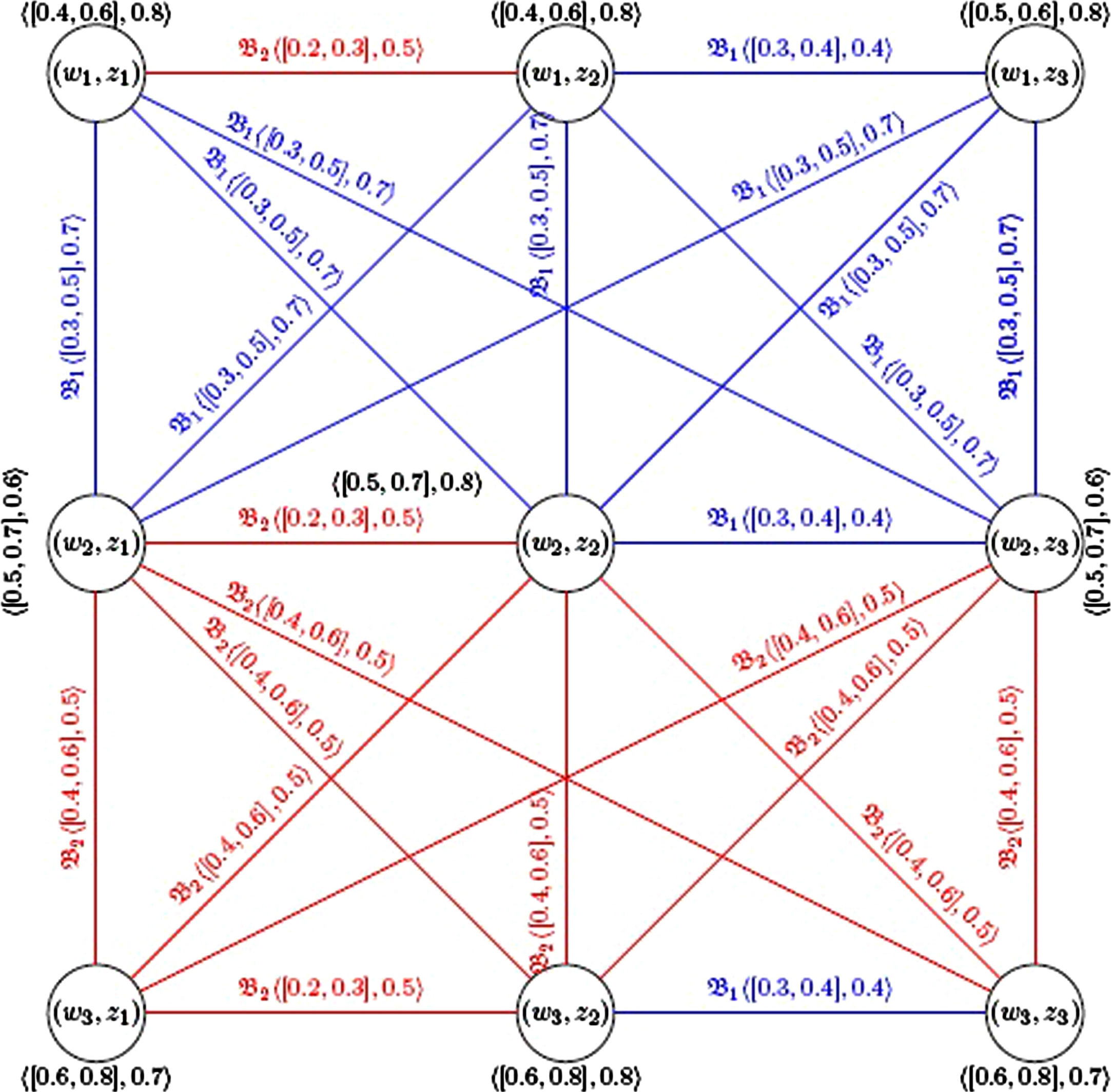
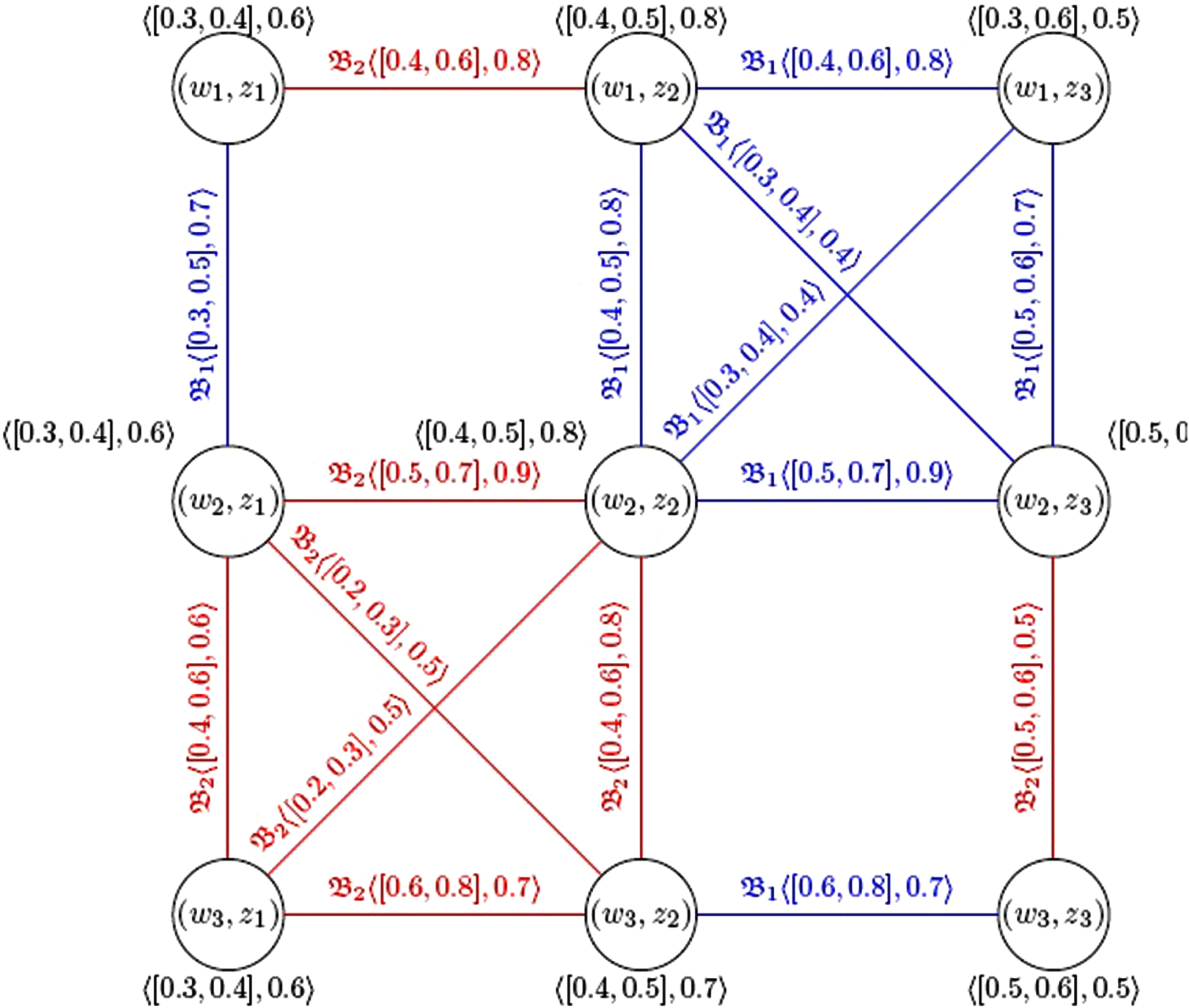
Example 3.1.2. Consider two CFGSs and , which are shown in Fig. 1.
CFGSs and .
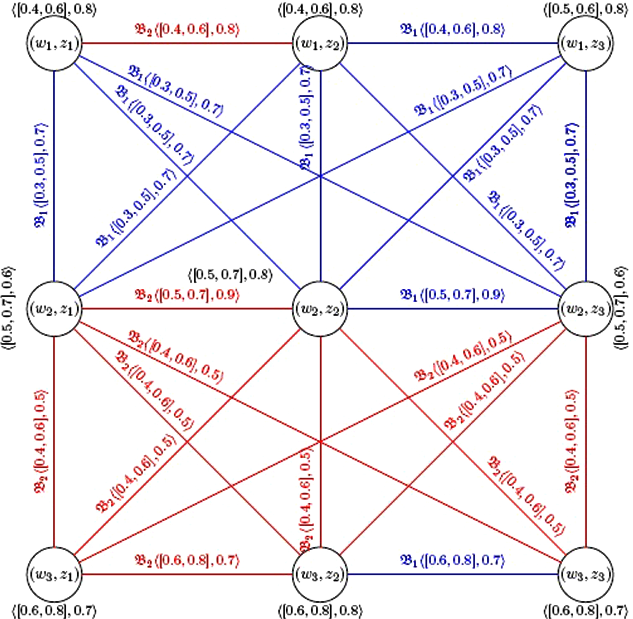
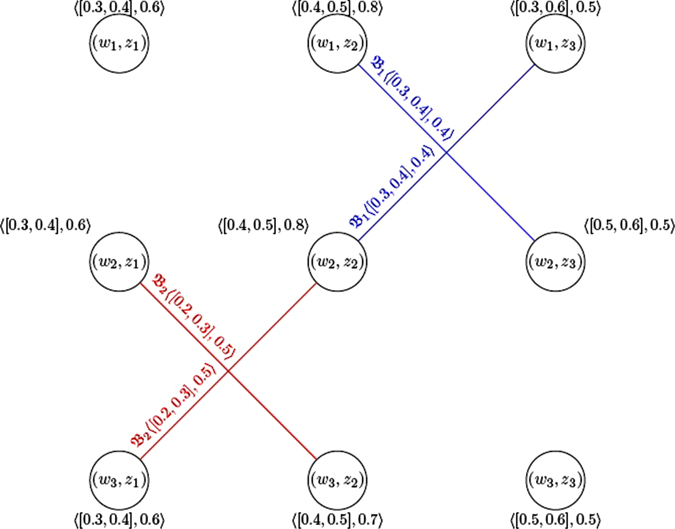
The lexicographic min-product of and is shown in Fig. 2.
The lexicographic min-product of two CFGSs of and , .
Remark 3.1.3. The lexicographic min-product operation of two CFGSs is not commutative. The lexicographic min-product of two strong CFGSs need not be strong. Also, the lexicographic min-product of two complete CFGSs need not be complete.
Theorem 3.1.4.If and are two CFGSs so that , , , and and are constant functions of the same value for i = 1, 2, ⋯ , k, then, the lexicographic min-product of and is a strong CFGS.
Proof. Let and be two CFGSs so that , , , and and are constant functions of the same value for i = 1, 2, ⋯ , k. Then, by the definition of the lexicographic min-product,
Case (i): w1w2 ∈ Ei. Then,
Case (ii): w1 = w2 and . Then,
Therefore, , for all edges of lexicographic min-product of and . Similarly,
Definition 3.1.5. The degree of a vertex in lexicographic min-product of two CFGSs and is defined as , where
-degree of a vertex of lexicographic min-product is determined as , where
Example 3.1.6. Consider the lexicographic min-product of two CFGSs and drawn in Fig. 2. The degree of vertex (w2, z2) in lexicographic min-product of is calculated as follows:
Therefore, the degree of vertex (w2, z2) in the lexicographic min-product is equal to .
-degree of vertex (w2, z2) of lexicographic min-product is determined as follows:
Therefore, the -degree of vertex (w2, z2) of lexicographic min-product is equal to .
Lexicographic max-product
Definition 3.2.1. Let and be two CFGSs with underlying crisp GSs G* = (V, E1, E2, ⋯ , Ek) and , respectively. Then, is named lexicographic max-product of and with underlying crisp GS , where, and , and it is defined as
for i = 1, 2, ⋯ , k.
Example 3.2.2. Consider two CFGSs of and , which are shown in Fig. 1.
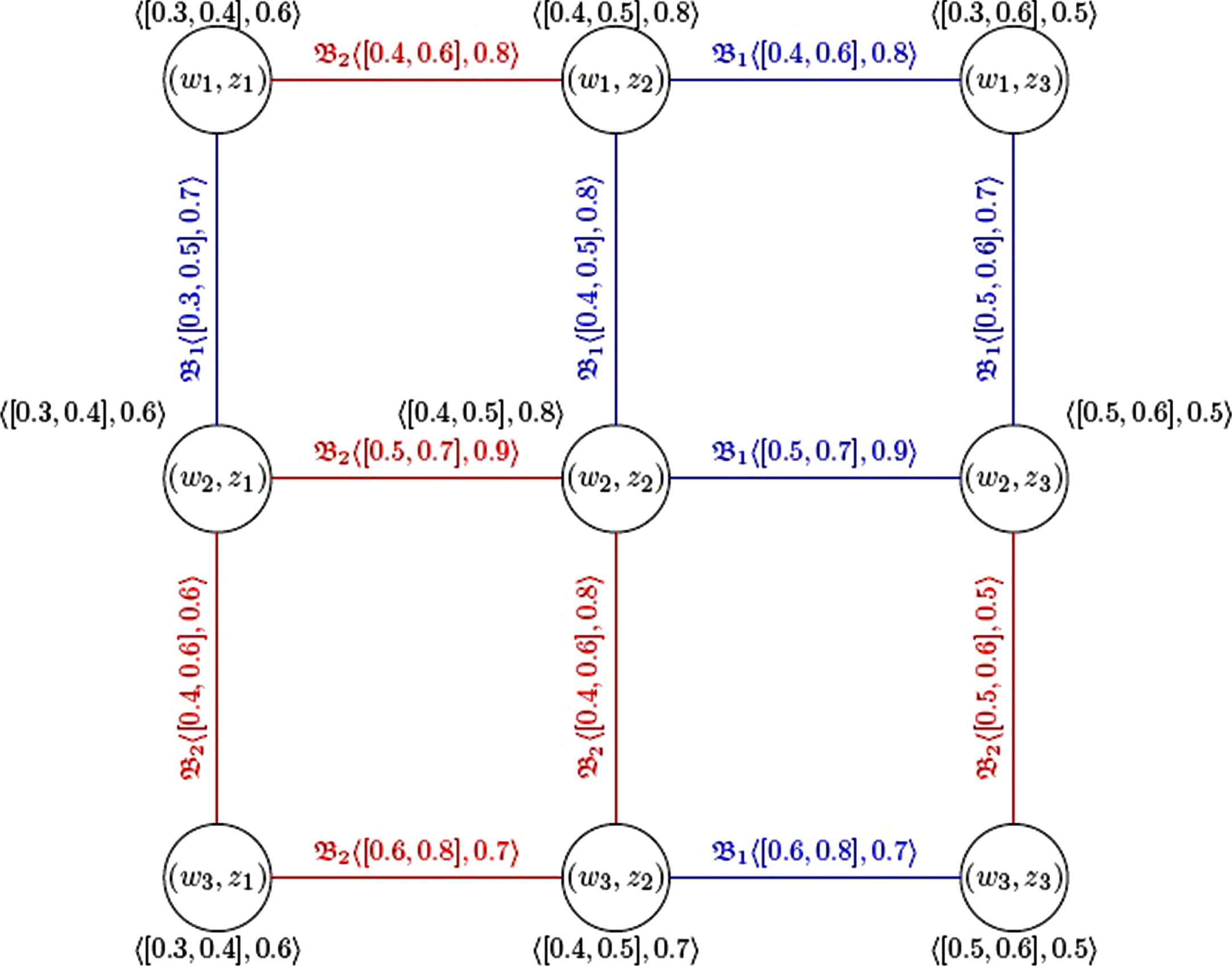
The lexicographic max-product of and is shown in Fig. 3.
The lexicographic max-product of two CFGSs of and , .
Remark 3.2.3. The lexicographic max-product operation of two CFGSs is not commutative. The lexicographic max-product of two strong CFGSs need not be strong. Also, the lexicographic max-product of two complete CFGSs need not be complete.
Definition 3.2.4. The degree of a vertex in lexicographic max-product of of two CFGSs of and is defined as , where
-degree of a vertex of lexicographic max-product is determined as , where
Example 3.2.5. Consider the lexicographic max-product of two CFGSs of and drawn in Fig. 3. The degree of vertex (w2, z2) in lexicographic max-product is calculated as follows:
Therefore, the degree of vertex (w2, z2) in the lexicographic max-product of is equal to .
-degree of vertex (w2, z2) of lexicographic max-product is determined as follows:
Therefore, the -degree of vertex (w2, z2) of lexicographic max-product of is equal to .
Maximal product
Definition 3.3.1. Let and be two CFGSs with underlying crisp GSs G* = (V, E1, E2, ⋯ , Ek) and , respectively. Then, is named maximal product of and with underlying crisp GS , where, and , and it is defined as
for i = 1, 2, ⋯ , k.
Example 3.3.2. Consider two CFGSs of and , which are shown in Fig. 1.
Theorem 3.3.3.The maximal product of two strong CFGSs is also a strong CFGS.
Proof. Let and be two CFGSs. Then, for any w1w2 ∈ Ei and for any , i = 1, 2, ⋯ , k. Then, by the definition of the maximal product,
Case (i): w1 = w2 and . Then,
Case (ii): z1 = z2 and w1w2 ∈ Ei. Then,
Therefore, for all edges of maximal product of and . Similarly,
Hence, is a strong CFGS. □
Definition 3.3.4. The degree of a vertex in the maximal product of of two CFGSs of and is defined as , where
-degree of a vertex of maximal product is determined as , where
Example 3.3.5. Consider the maximal product of two CFGSs of and drawn in Fig. 3. The degree of the vertex (w2, z2) in the maximal product is calculated as follows:
Therefore, the degree of vertex (w2, z2) in the maximal product is equal to .
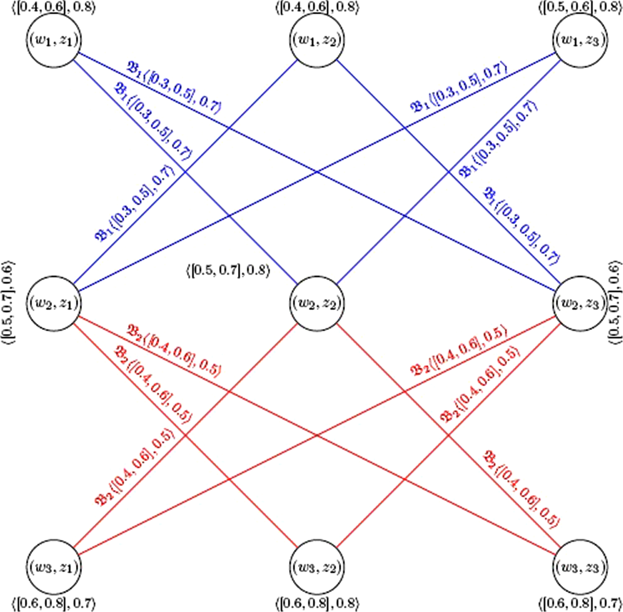
The residue product of two CFGSs of and , .
-degree of vertex (w2, z2) of maximal product of is determined as follows:
Therefore, the -degree of vertex (w2, z2) of maximal product is equal to .
Residue product
Definition 3.4.1. Let and be two CFGSs with underlying crisp GSs G* = (V, E1, E2, ⋯ , Ek) and , respectively. Then, is named residue product of and with the underlying crisp GS , where, and , and it is defined as
for i = 1, 2, ⋯ , k.
Example 3.4.2. Consider two CFGSs and , which are shown in Fig. 1.
Theorem 3.4.3.If is a strong CFGS and is any CFGS so that , , , for i = 1, 2, ⋯ , k, then, the residue product of and is a strong CFGS.
Proof. Let be a strong CFGS and be any CFGS so that , , , for i = 1, 2, ⋯ , k. Then, by the definition of the residue product,
If w1w2 ∈ Ei, z1 ≠ z2, then,
Therefore, , for all edges of residue product of and . Similarly,
Hence, is a strong CFGS. □
Definition 3.4.4. The degree of a vertex in residue product of of two CFGSs of and is defined as , where
-degree of a vertex of residue product is determined as , where
Example 3.4.5. Consider the residue product of two CFGSs of and drawn in Fig. 1. The degree of vertex (w2, z2) in residue product of is calculated as follows:
Therefore, the degree of vertex (w2, z2) in the residue product of is equal to .
-degree of vertex (w2, z2) of residue product of is determined as follows:
Therefore, the -degree of vertex (w2, z2) of residue product of is equal to .
Strong product
Definition 3.5.1. Let and be two CFGSs with underlying crisp GSs G* = (V, E1, E2, ⋯ , Ek) and , respectively. Then, is named the strong product of and with underlying crisp GS , where, and , and it is defined as
The strong product two CFGSs of and , .
for i = 1, 2, ⋯ , k.
Example 3.5.2. Consider two CFGSs and , which are shown in Fig. 1.
Theorem 3.5.3.If and are two strong CFGSs, then, the strong product of and is a strong CFGS.
Proof. Let and be two CFGSs. Then, for any w1w2 ∈ Ei and for any , i = 1, 2, ⋯ , k. Thus, by the definition of the strong product,
Case (i): w1 = w2 and . Then,
Case (ii): z1 = z2 and w1w2 ∈ Ei. Then,
Case (iii): . Then,
Therefore, for all edges of the strong product of and . Similarly,
Hence, is a strong CFGS. □
Definition 3.5.4. The degree of a vertex in the strong product of of two CFGSs and is defined as , where
-degree of a vertex of the strong product of is determined as , where
Example 3.5.5. Consider the strong product of two CFGSs of and drawn in Fig. 6. The degree of vertex (w2, z2) in the strong product of is calculated as follows:
Therefore, the degree of vertex (w2, z2) in the strong product of is equal to .
-degree of vertex (w2, z2) of the strong product of is determined as follows:
Therefore, the -degree of vertex (w2, z2) of the strong product of is equal to .
Cartesian product
Definition 3.6.1. Let and be two CFGSs with underlying crisp GSs G* = (V, E1, E2, ⋯ , Ek) and , respectively. Then, is named the Cartesian product of and with underlying crisp GS , where, and , and it is defined as
for i = 1, 2, ⋯ , k.
Example 3.6.2. Consider two CFGSs of and , which are shown in Fig. 1.
Theorem 3.6.3.The Cartesian product of two strong CFGSs is also a strong CFGS.
Proof. Similar to the above theorems, it can be easily proved. □
Definition 3.6.4. The degree of a vertex in Cartesian product of two CFGSs and is defined as , where
-degree of a vertex of the Cartesian product of is determined as , where
Example 3.6.5. Consider the Cartesian product of two CFGSs and drawn in Fig. 6. The degree of the vertex (w2, z2) in the Cartesian product of is calculated as follows:
Therefore, the degree of the vertex (w2, z2) in the Cartesian product of is equal to .
-degree of the vertex (w2, z2) of the Cartesian product of is determined as follows:
Therefore, the -degree of the vertex (w2, z2) of the Cartesian product of is equal to .
Tensor product
Definition 3.7.1. Let and be two CFGSs with the underlying crisp GSs of G* = (V, E1, E2, ⋯ , Ek) and , respectively. Then, is named the tensor product of and with the underlying crisp GS of , where, and , and it is defined as
for i = 1, 2, ⋯ , k.
Example 3.7.2. Consider two CFGSs of and , which are shown in Fig. 1.
Theorem 3.7.3.If and are two strong CFGSs, then, the tensor product of and is a strong CFGS.
Proof. Let and be two CFGSs. Then, for any w1w2 ∈ Ei and for any , i = 1, 2, ⋯ , k. Thus, by the definition of the tensor product,
If , then,
Therefore, for all edges of the tensor product and . Similarly,
Hence, is a strong CFGS. □
Definition 3.7.4. The degree of a vertex in the tensor product of of two CFGSs of and is defined as , where
-degree of a vertex of the tensor product of is determined as , where
Example 3.7.5. Consider the tensor product of two CFGSs and drawn in Fig. 8. The degree of the vertex (w2, z2) in the tensor product of is calculated as follows:
Therefore, the degree of the vertex (w2, z2) in the tensor product of is equal to .
-degree of the vertex (w2, z2) of the tensor product of is determined as follows:
Therefore, the -degree of the vertex (w2, z2) of the tensor product of is equal to .
Direct sum
Definition 3.8.1. Let and be two CFGSs with an underlying crisp GSs of G* = (V, E1, E2, ⋯ , Ek) and , respectively. Then, is named direct sum of and with the underlying crisp GS , where, and , and it is defined as
for i = 1, 2, ⋯ , k.
Example 3.8.2. Consider two CFGSs of and , which are shown in Fig. 1, so that w2 = z2.
Theorem 3.8.3.If and are two strong CFGSs so that no edge of has both ends in V ∩ V′ and every edge wz of with one end w ∈ V ∩ V′ and is so that , then is a strong CFGS.
Proof. Let and be two CFGSs. Let wz be an edge of . Then,
Case (i): wz ∉ V ∩ V′. Then, w, z ∈ VorV′ but not both. Assume that w, z ∈ V. Then, wz ∈ E. Therefore, , , and , , . Also, , , . Since is a strong CFGS, then
A similar argument exists for w, z ∈ V′.
Case (ii): w ∈ V ∩ V′ and z ∉ V ∩ V′ (or vice versa). Without the loss of generality, assume that z ∈ V. Then, , , . By such hypothesis, . Thus,
So, . Similarly, , . Therefore,
Hence, is a strong CFGS. □
Definition 3.8.4. The degree of a vertex in the direct sum of two CFGSs and is defined as follows
-degree of a vertex of the direct sum of is determined as follows
Example 3.8.5. Consider the direct sum of two CFGSs of and drawn in Fig. 9. The degree of the vertex (w2) in the direct sum is calculated as follows:
Therefore, the degree of the vertex (w2) in the direct sum of is equal to .
-degree of a vertex (w2) of the direct sum of is determined as follows:
Therefore, the -degree of vertex (w2) of direct sum is equal to .
The relationship between products
In the following, we introduce some relationships between products.
Theorem 3.9.1.The lexicographic min-product of of two CFGSs of and is a spanning cubic fuzzy sub graph structure of the lexicographic max-product of .
Proof. Consider the lexicographic max-product of . and lexicographic min-product of two CFGSs and . From the definitions of the lexicographic max-product, and the lexicographic min-product, it is clear that for all (w1, z1) ∈ V × V′, and , for all . Therefore, and . Hence, the lexicographic min-product is a spanning cubic fuzzy sub graph structure of the lexicographic max-product. □
Example 3.9.2. The lexicographic min-product of , drawn in Fig. 2, is a spanning cubic fuzzy sub graph structure of the lexicographic max-product of which is drawn in Fig. 3.
Theorem 3.9.3.If and are two CFGSs so that , , , for i = 1, 2, ⋯ , k, then,
That is, the lexicographic max-product of and is the direct sum of the maximal product and the residue product of two CFGSs.
Proof. Let and be two CFGSs so that , , , for i = 1, 2, ⋯ , k. Then, , , . Consider . According to the definitions of maximal product, residue product, and lexicographic max-product we have . Then,
Therefore, is actually the lexicographic max-product of of and . Thus,
□
Corollary 3.9.4.If and are two CFGSs such that , , , for i = 1, 2, ⋯ , k, then,
Proof. The proof is similar to the above theorem.□
Theorem 3.9.5.If and are two CFGSs, then,
That is, the strong product of two CFGSs of and is the direct sum of the Cartesian product and the tensor product of and .
Proof. Let and be two CFGSs. According to the definitions of the operators, we have
for every (w, z) ∈ V × V′. Therefore,
Thus,
According to the definitions of the Cartesian product and tensor product, we will have
for i = 1, 2, ⋯ , k. Therefore,
□
The application
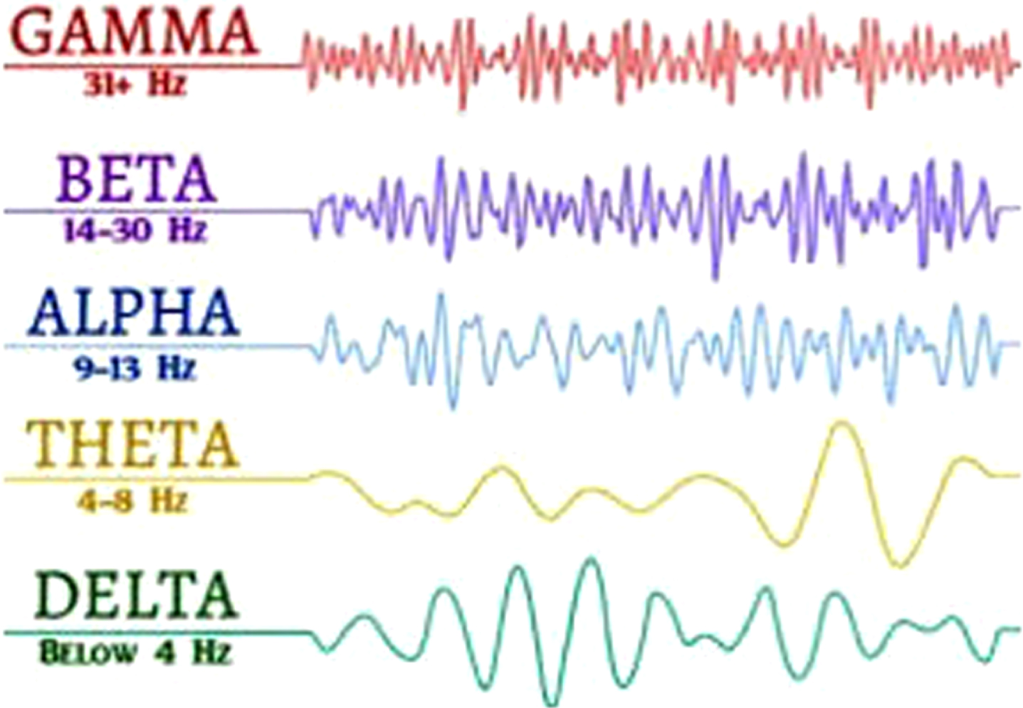
The human brain is the most complex structure in the world, which has 100 billion nerve cells. These cells are busy with work and activity at every moment of time, which results in the formation of behaviors, feelings and thoughts. Each person has 5 different types of brain waves, which are gamma (γ), beta (β), alpha (α), theta (θ) and delta (δ) according to Fig. 10. While all brain waves work simultaneously, one brain wave can be more dominant and active than the others. The dominant brain wave determines the current mental state of the person. Injuries such as seizures, encephalitis, anxiety, depression, learning disorders, obsessive-compulsive disorder, etc. cause brain wave activity to change. In this way, many abnormalities and abnormal functions of the brain can be identified and appropriate measures can be taken to treat them. Different patterns of electrical activity, known as brain waves, can be identified by their amplitude and frequency. Frequency indicates how quickly the waves are changing, measured by the number of waves per second, while amplitude measures the strength of these waves, measured by microvolts.
Brain waves.
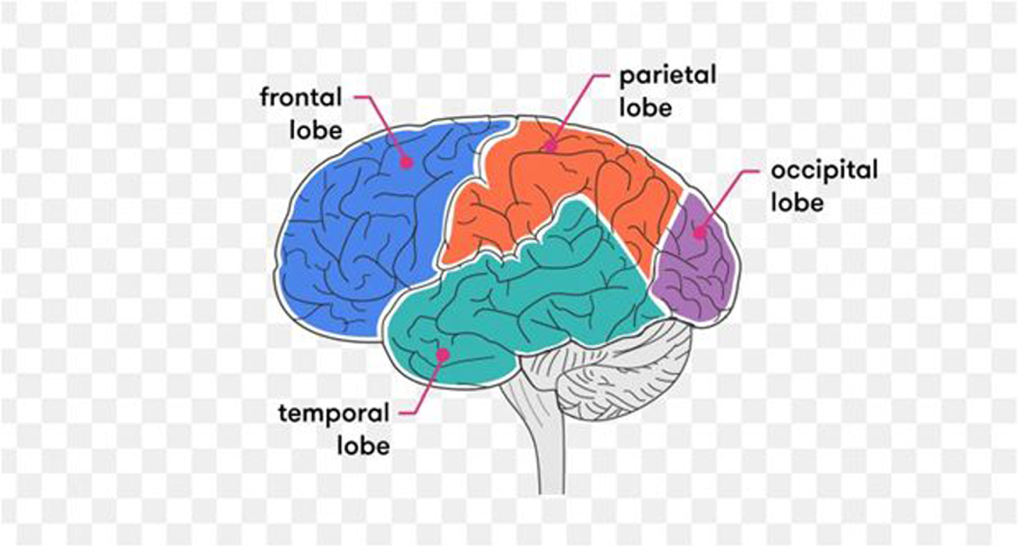
The cerebrum is the largest part of the brain, which consists of four distinct lobes: frontal, temporal, parietal, and occipital according to Fig. 11. Each of these lobes has different functions, some of which may overlap. The cerebrum can be anatomically divided into two parts: the right and left hemispheres.
Lobes of the brain.
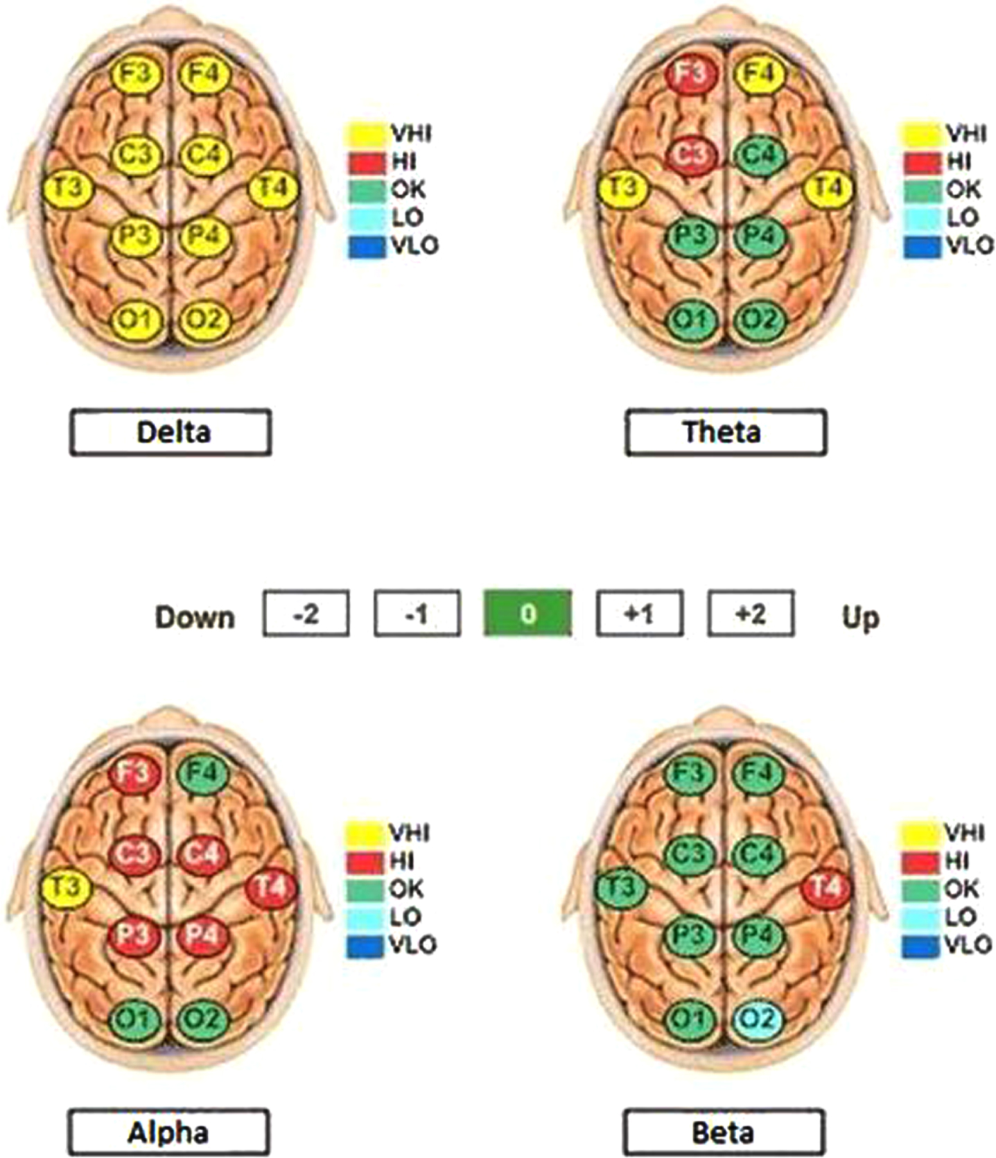
We considered ten regions of the brain according to the international standard 10-20 system, which are the locations of electrodes on the head surface during brain electroencephalography recording. Figure 12 shows a report of the brain map related to the activity of brain waves in each lobe of the brain. The letters F, P, T, O, and C correspond to the frontal, partial, temporal, occipital, and central regions, respectively. On a brain map, green usually indicates normal activity levels, red indicates high levels, and yellow indicates extreme levels of activity.
Brain map related to the activity of brain waves in each lobe.
Absolute power measurement aids the neurotherapist in determining whether enough brainpower within a particular frequency range is present at each recording site. The relative power measurement aids the neurotherapist in determining whether a particular frequency is overpowering other vital brain frequencies. The average absolute power and relative power of the four brain waves of alpha, beta, theta and delta in an EEG test are shown in Table 2. A CFGS can be useful in diagnosing certain abnormalities in the brain. For this purpose, we consider the points identified in the lobes of the brain as vertices. The cubic fuzzy values of the vertices are given in Table 3. In this table, the average relative power is presented as a number with an interval value.
Average absolute power and relative power of brain waves in each lobe
Lobe
Average absolute power
Average relative power
F3
58
45
F4
60
56
C3
30
28
C4
35
33
T3
50
47
T4
45
42
P3
40
39
P4
43
40
O1
57
55
O2
55
52
Cubic fuzzy values of lobes
Lobe
Cubic fuzzy value
F3
〈[0.79, 0.81] , 0.96〉
F4
[0.90, 1] , 1
C3
〈[0.49, 0.51] , 0.50〉
C4
〈[0.57, 0.59] , 0.58〉
T3
〈[0.82, 0.84] , 0.83〉
T4
〈[0.74, 0.76] , 0.75〉
P3
〈[0.68, 0.70] , 0.66〉
P4
〈[0.70, 0.72] , 0.71〉
O1
〈[0.97, 0.99] , 0.95〉
O2
〈[0.91, 0.93] , 0.91〉
The relationship between the lobes in Fig. 12 is one of the types of brain waves that are more or less than normal. It is clear that the regions of different colors are connected as long as they have the highest frequency compared to other waves. Green vertices are not connected because they represent the normal surface of the wave. The cubic fuzzy values and the dominant wave in the connection between different regions of the lobes are shown in Table 4. Since the most dominant wave is considered between two vertices, then all edges are strong.
The cubic fuzzy values of relations between two lobes
The relationship between the lobes
Brain wave
Cubic fuzzy value
F3 - F4
Delta
〈[0.79, 0.81] , 0.96〉
C3 - C4
Alpha
〈[0.49, 0.51] , 0.50〉
F3 - C4
Alpha
〈[0.57, 0.59] , 0.58〉
C3 - F4
Delta
〈[0.49, 0.51] , 0.50〉
C3 - P4
Alpha
〈[0.49, 0.51] , 0.50〉
P3 - C4
Alpha
〈[0.57, 0.59] , 0.58〉
P3 - P4
Alpha
〈[0.68, 0.70] , 0.66〉
P3 - O2
Delta
〈[0.68, 0.70] , 0.66〉
O1 - P4
Delta
〈[0.70, 0.72] , 0.71〉
O1 - O2
Delta
〈[0.91, 0.93] , 0.91〉
F3 - C3
Alpha
〈[0.49, 0.51] , 0.50〉
F4 - C4
Delta
〈[0.57, 0.59] , 0.58〉
C3 - P3
Alpha
〈[0.49, 0.51] , 0.50〉
C4 - P4
Alpha
〈[0.57, 0.59] , 0.58〉
O1 - P3
Delta
〈[0.68, 0.70] , 0.66〉
O2 - P4
Delta
〈[0.70, 0.72] , 0.71〉
T3 - F3
Delta
〈[0.79, 0.81] , 0.83〉
T3 - C3
Delta
〈[0.49, 0.51] , 0.50〉
T3 - P3
Delta
〈[0.68, 0.70] , 0.66〉
T3 - O1
Delta
〈[0.82, 0.84] , 0.83〉
T4 - F4
Theta
〈[0.74, 0.76] , 0.75〉
T4 - C4
Alpha
〈[0.57, 0.59] , 0.58〉
T4 - P4
Alpha
〈[0.70, 0.72] , 0.71〉
T4 - O2
Delta
〈[0.74, 0.76] , 0.75〉
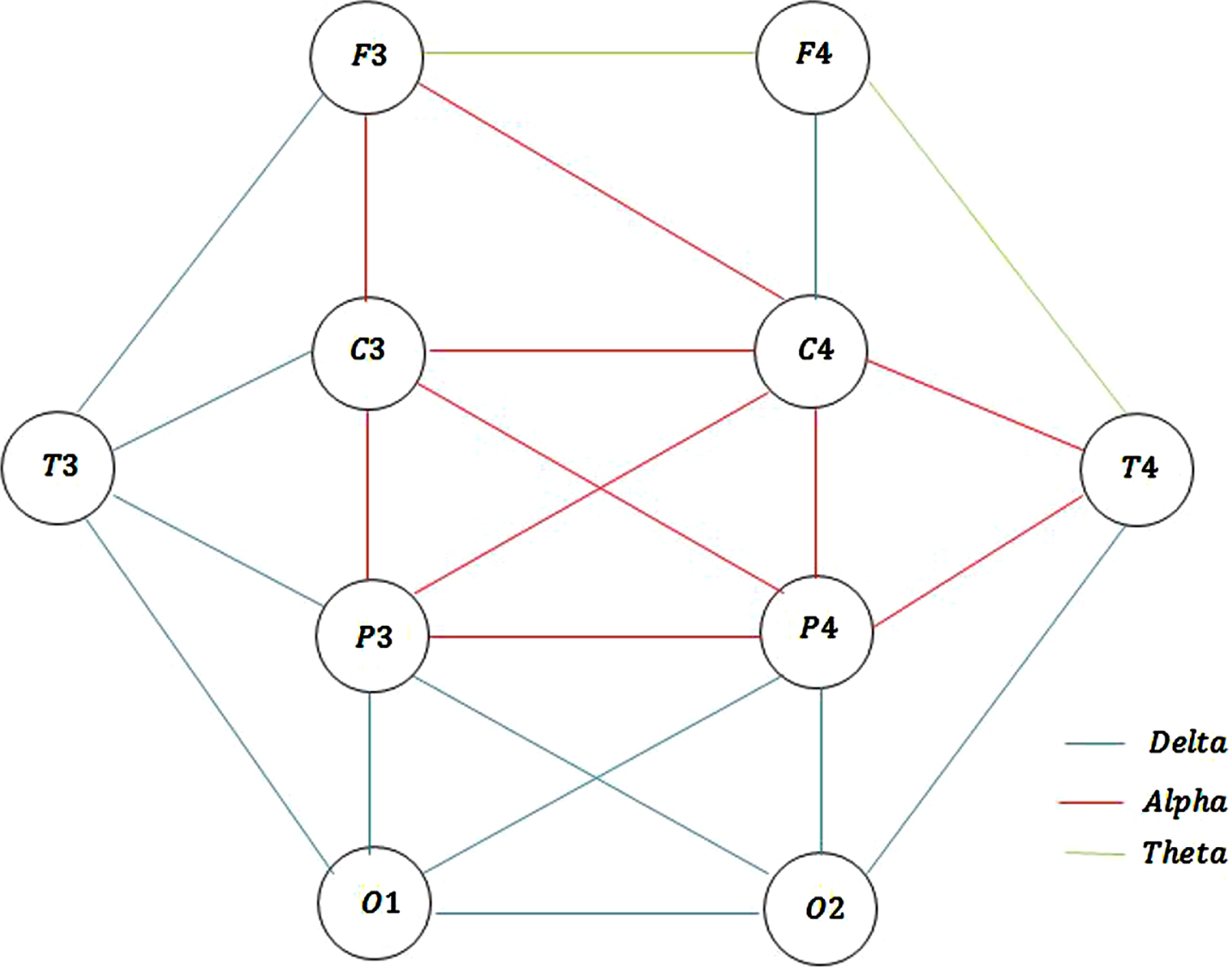
Therefore, we will have a CFGS with the following defined relations:
The CFGS with three relations of delta, theta, and alpha are drawn in Fig. 13.
The CFGS .
Figure 13 shows brain waves at an abnormal level and the areas of the brain that are involved in these waves. Areas that are affected by several waves with very low or very high intensity are considered dangerous. In this way, it is easy to find a disorder in the brain and take the necessary measures.
Compared to the usual methods, this method facilitates the analysis of brain disorders by weighting the lobes and the connections between them. Also, the use of graph parameters such as the connection between the lobes and the calculation of the closest distance between them can be useful in the diagnosis and treatment of brain disorders. The outlook for people with brain disorders depends on the type and severity of the brain disorder. Some diseases are easily cured with medicine and other treatments. For example, millions of people with mental disorders completely lead normal lives. Other disorders, such as neurological diseases and some traumatic brain injuries, have no cure. People with these conditions often experience permanent changes in their behavior, mental abilities, or coordination. Calculations based on this method help people to manage their disease and maintain their health as much as possible.
Conclusions
Cubic fuzzy graph structure (CFGS) as a combination of fuzzy graph structure and cubic fuzzy graph, has better flexibility in modeling and solving problems in ambiguous and uncertain fields. In this article, we introduced some of the most important product operations on CFGSs and examined their characteristics. The results showed that the product of two strong CFGSs is not always strong. Some of them will be strong under certain conditions. Calculating the degree in the product of two CFGSs and comparing them in this study has been quite evident. These degrees are expressed as a cubic number so that it is possible to compare the products easily. It was found that the conditions of membership functions between two CFGSs are effective in the quality of the degree calculation. Also, in a novel way, we have discussed the relations between product operations and we have reached interesting results. It is known that the combination of some products results in other products. At the end, the CFGS application in the diagnosis of brain lesions is presented. In our future work, we intend to express its specialized features by relying on a special type of product operation and vertex regularity on CFGSs.
References
1.
ZadehL.A., Fuzzy sets, Information and control8 (1965), 338–353.
2.
KauffmanA., Introduction a la Theorie des Sous-Emsembles Flous, Masson: Issy-les-Moulineaux, French, 1 (1973).
3.
RosenfeldA., Fuzzy Graphs, Fuzzy Sets and Their Applications, Academic Press, NewYork, NY, USA, (1975), 77–95.
4.
TalebiA.A., Cayley fuzzy graphs on the fuzzy group, Computational and Applied Mathematics37(4) (2018), 4611–4632.
5.
BorzooeiR.A. and RashmanlouH., New concepts of vague graphs, International Journal of Machine Learning and Ceybernetics8(4) (2016), 1081–1092.
6.
BorzooeiR.A., RashmanlouH., SamantaS. and PalM., Regularity of vague graphs, Journal of Intelligent and Fuzzy Systems30 (2016), 3681–3689.
7.
AtanassovK., Intuitionistic fuzzy sets, Fuzzy Sets and Systems20 (1986), 87–96.
8.
AkramM. and DudekW.A., Interval-valued fuzzy graphs, Computers & Mathematics with Applications61(2) (2011), 289–299.
9.
TalebiA.A., RashmanlouH. and SadatiS.H., New concepts on m-polar interval-valued intuitionistic fuzzy graph, TWMS J Appl Eng Math10(3) (2020), 808–816.
10.
TalebiA.A., RashmanlouH. and SadatiS.H., Interval-valued Intuitionistic Fuzzy Competition Graph, Journal of Multiple-Valued Logic & Soft Computing34 (2020), 335–364.
11.
KosariS., RaoY., JiangH., LiuX., WuP. and ShaoZ., Vague graph structure with application in medical diagnosis, Symmetry12(10) (2020), 15–82.
12.
RaoY., KosariS. and ShaoZ., Certain properties of vague graphs with a novel application, Mathematics8(10) (2020), 1647.
13.
KouZ., KosariS. and AkhoundiM., A Novel Description on Vague Graph with Application in Transportation Systems, Journal of Mathematics (2021), 11 pages. doi: 10.1155/2021/4800499.
14.
RaoY., KosariS., ShaoZ., CaiR. and XinyueL., A study on domination in vague incidence graph and its application in medical sciences, Symmetry12(11) (2020), 18–85.
15.
RaoY., KosariS., ShaoZ., QiangX., AkhoundiM. and ZhangX., Equitable Domination in Vague Graphs With Application in Medical Sciences, Frontiers in Physics37 (2021), doi: 10.3389/fphy.2021.635642
16.
ShiX. and KosariS., Certain Properties of Domination in Product Vague Graphs With Novel Application in Medicine, Frontiers in Physics9 (2021), 3–85.
17.
ShaoZ., KosariS., RashmanlouH. and ShoaibM., New concepts in intuitionistic fuzzy graph with application in water supplier systems, Mathematics8(8) (2020), 12–41.
18.
BorzooeiR.A. and RashmanlouH., Ring sum in product intuitionistic fuzzy graphs, Journal of Advanced Research in Pure Mathematics7(1) (2015), 16–31.
19.
SampathkumarE., Generalized graph structures, Bull Kerala Math Assoc3(2) (2006), 65–123.
20.
DineshT., A study on graph structures, incidence algebras and their fuzzy analogues, Ph.D. Thesis, Kannur University, Kannur (2011), India.
21.
DineshT. and RamakrishnanT., On generalised fuzzy graph structures, Applied Mathematical Sciences5(4) (2011), 173–180.
22.
AkramM., m–polar fuzzy graph structures, In: m-polar fuzzy graphs, Studies in fuzziness and soft computing, Springer, Springer, Cham371 (2019), 209–233.
23.
AkramM. and AkmalR., Application of bipolar fuzzy sets in graph structures, Applied Computational Intelligence and Soft Computing, 2016.
24.
AkramM. and AkmalR., Intuitionistic fuzzy graph structures, Kragujevac Journal of Mathematics41(2) (2017), 219–237.
25.
AkramM. and AkmalR., Operations on intuitionistic fuzzy graph structures, Fuzzy Information and Engineering8(4) (2016), 389–410.
26.
AkramM. and SitaraM., Certain fuzzy graph structures, Journal of Applied Mathematics and Computing61(1) (2019), 25–56.
27.
SitaraM., AkramM. and Yousaf BhattiM., Fuzzy graph structures with application, Mathematics7(1) (2019), 63.
28.
AkramM., SitaraM. and SaeidA.B., Residue product of fuzzy graph structures, Journal of Multiple-Valued Logic and Soft Computing34 (2020), 365–399.
29.
KoamA.N., AkramM. and LiuP., Decision-making analysis based on fuzzy graph structures, Mathematical Problems in Engineering, 2020.
30.
AkramM. and SitaraM., Novel applications of single-valued neutrosophic graph structures indecision-making, Journal of Applied Mathematics and Computing56(1) (2018), 501–532.
31.
KouZ., AkhoundiM., ChenX. and OmidiS., A study on vague graph structures with anapplication, Advances in Mathematical Physics, 2022.
AkramM. and SitaraM., Decision-making with q-rung orthopair fuzzy graph structures, Granular Comput 2021. doi: 10.1007/s41066-021-00281-3
34.
SitaraM. and ZafarF., Selection of best inter-country airline service using q-rung picture fuzzy graph structures, Computational and Applied Mathematics41(1) (2022), 1–32.
35.
JunY.B., KimC.S. and YangK.O., Cubic sets, Ann Fuzzy Math Inform4(1) (2012), 83–98.
36.
JunY.B., SmarandacheF. and KimC.S., Neutrosophic cubic sets, New Mathematics and Natural Computation13(01) (2017), 41–54.
37.
JunY.B., SongS.Z. and KimS.J., Cubic interval-valued intuitionistic fuzzy sets and their application in BCK/BCI-algebras, Axioms7(1) (2018), 7.
38.
JunY.B., LeeK.J. and KangM.S., Cubic structures applied to ideals of BCI-algebras, Computers & Mathematics with Applications62(9) (2011), 3334–3342.
39.
KhanM., JunY.B., GulistanM. and YaqoobN., The generalized version of Jun’s cubic sets in semigroups, Journal of Intelligent & Fuzzy Systems28(2) (2015), 947–960.
40.
AliA., JunY.B., KhanM., ShiF.G. and AnisS., Generalized cubic soft sets and their applications to algebraic structures, Italian Journal of Pure and Applied Mathematics35 (2015), 393–414.
41.
SenapatiT., JunY.B., MuhiuddinG. and ShumK.P., Cubic intuitionistic structures applied to ideals of BCI-algebras, Analele Stiintifice ale Universitatii Ovidius Constanta-Seria Matematica27(2) (2019), 213–232.
KrishnaK.K., RashmanlouH., TalebiA.A. and MofidnakhaeiF., Regularity of cubic graph with application, Journal of the Indonesian Mathematical Society (2019), 1–15.
44.
RashidS., YaqoobN., AkramM. and GulistanM., Cubic graphs with application, International Journal of Analysis and Applications16(5) (2018), 733–750.
45.
MuhiuddinG., TakalloM.M., JunY.B. and BorzooeiR.A., Cubic graphs and their application to a traffic flow problem, International Journal of Computational Intelligence Systems13(1) (2020), 1265–1280.
46.
RashmanlouH., MuhiuddinG., AmanathullaS.K., MofidnakhaeiF. and PalM., A study on cubic graphs with novel application, Journal of Intelligent & Fuzzy Systems40(1) (2021), 89–101.
47.
JiangH., TalebiA.A., ShaoZ., SadatiS.H. and RashmanlouH., New Concepts of Vertex Covering in Cubic Graphs with Its Applications, Mathematics10(3) (2022), 307.
48.
ShiX., AkhoundiM., TalebiA.A. and SadatiS.H., Some Properties of Cubic Fuzzy Graphs with an Application, Symmetry14(12) (2022), 2623.
49.
GulistanM., AliM., AzharM., RhoS. and KadryS., Novel neutrosophic cubic graphs structures with application in decision making problems, IEEE access7 (2019), 94757–94778.
50.
MuhiuddinG., AlanaziA.M., MahboobA., AlkhaldiA.H. and AlatwaiW., A Novel Study of Graphs Based on m-Polar Cubic Structures, Journal of Function Spaces (2022), 2022.
51.
RaoY., AkhoundiM., TalebiA.A. and SadatiS.H., The Maximal Product in Cubic Fuzzy Graph Structures with an Application, International Journal of Computational Intelligence Systems16(1) (2023), 18.