Feature extraction of linear separability using robust autoencoder with distance metric

Abstract

This paper proposes a robust autoencoder with Wasserstein distance metric to extract the linear separability features from the input data. To minimize the difference between the reconstructed feature space and the original feature space, using Wasserstein distance realizes a homeomorphic transformation of the original feature space, i.e., the so-called the reconstruction of feature space. The autoencoder is used for features extraction of linear separability in the reconstructed feature space. Experiment results on real datasets show that the proposed method reaches up 0.9777 and 0.7112 on the low-dimensional and high-dimensional datasets in extracted accuracies, respectively, and also outperforms competitors. Results also confirm that compared with feature metric-based methods and deep network architectures-based method, the linear separabilities of those features extracted by distance metric-based methods win over them. More importantly, the linear separabilities of those features obtained by evaluating distance similarity of the data are better than those obtained by evaluating feature importance of data. We also demonstrate that the data distribution in the feature space reconstructed by a homeomorphic transformation can be closer to the original data distribution.

Keywords

Autoencoder distance measure feature extraction linear separability

1 Introduction

Feature extraction aims at seeking the valuable features from the data through filtering redundant information [1, 2]. Many factors can affect feature extraction, such as data dimension, data distribution, etc. From the perspective of data dimension, feature extraction becomes more and more difficulty as the dimension increases, since the data is sparse distribution upon a high-dimensional space, it is hard to afford sufficient information. However, feature extraction relies on the data information. Form the view of data distribution, usually, the data distribution is unknown and complex, which bring challenges for extracted approaches. Additional, linear separability of those extracted features are used for an evaluated metric aiming at the results of feature extraction [3]. Therefore, feature extraction of the data is a tough work.

Recently, some efforts have been proposed for feature extraction, such as distance metric-based methods, feature metric-based methods, and deep network architectures-based methods. As follows,

Distance metric-based methods. The distance between the data has many types, such as, Mahalanobis distance, Wasserstein distance, Bhattacharyya distance, etc., but such methods adopt the manner of assessing the similarity between the data by the distance between the data. Through changing the distance between the data, the linear separability between features can be increased, i.e., the margins between features can be enlarged. For instance, the [4] proposed the intrinsic semi-supervised metric learning (ISSML) with a distance metric. Similarly, the [5] proposed the information-theoretic metric learning is (ITML) by employing a distance metric. And the [6] et al proposed a deep extraction method using Mahalanobis distance. Results show that the m-AE in [6] has greater advantages than the ISSML in [4] and the ITML in [5] in the linear separability of the extracted features. However, there are still issues in them, for instance, iterative optimization issues need to be addressed during feature extraction, furthermore, feature extraction significantly relies on parameter for them. In fact, distance metric-based methods may suffer from the dear calculation cost because of calculating distances between the data.

Feature metric-based methods. Such methods fully consider feature subsets of the data, and calculate feature subsets to achieve feature extraction. In terms of extracted accuracy, such methods indeed gain more since relative important features can be discovered via observing feature subsets. For instance, the [7] proposed a feature selection method with k-means through calculating a cluster of each feature subset, and fully utilizes feature relevance in the process of feature extraction. Unfortunately, calculating a cluster of each feature subset spends dear, particularly, calculation cost hardly affords for high dimensionality data or big scale data. In addition, also including LLE (locally linear embedding) [8], multi-manifold discriminant (MMD) isometric feature mapping [8], ISOMAP-KL [9]. The methods in [7 –9] rely on eigen decomposition, but eigen decomposition suffers from the embarrassment of being helpless when encountering singular matrices. Because of measuring feature relevance or importance, feature metric-based methods are favored when tending to extracted accuracy, while it is difficult for them to take into account the linear separability of extracted features. More difficult, how feature relevance or importance is assessed.

Deep network architecture-based methods. Usually, feature extraction can be considered to be dimension reduction of the data, so in this regard, deep network architecture-based methods have outstanding ascendency. One of classic representatives in such methods is an autoencoder architecture(AE)-based method, which is a dimension reduction method for the unknown meaningful insights [10], such as Logic-Oriented and Granular Logic Autoencoders in [11], providing the interpretable results, and Denoising Autoencoder [12], filtering noise hidden in the data, and the Sparse Autoencoder (SAE) [13], as well as, the Stacked Sparse Autoencoder (SSAE) [14]. These features extracted by these autoencoders have limitation in linear separability, since these loss functions in these autoencoders think more about extracted precision instead of considering the margins between the extracted features, so that the linear separabilities of features extracted by them are poor.

Motivation. The primary motivation of this work is to extract the features of linear separability from the data. The final purpose is to provide some insights for feature extraction, as well as give an evaluation regarding those methods of feature extraction. Therefore, here proposes a robust autoencoder with Wasserstein distance. To minimize the difference between the original feature space and the reconstructed feature space, a homeomorphic transformation of the original feature space is achieved through calculating Wasserstein distance, i.e., the reconstruction of feature space. In the reconstructed feature space, the autoencoder is used for features extraction with linear separability.

Contributions. We summarize the contributions of this works, as following.

A roust autoencoder with Wasserstein distance is proposed to obtain those features of linear separability.

The linear separabilities of features obtained by evaluating distance similarity between the data are better than these obtained by evaluating feature importance between the data.

The data distribution in the feature space reconstructed by a homeomorphic transformation can be closer to these in the original space.

2 Methodology

2.1 Reconstruction of feature space

To reconstruct the feature space, here, we need to introduce a transformation both feature spaces. The [3] interprets the transformation from a feature space to another one from the point of view of probability distribution, as follows.

The [3]. Given a convex region $Ω \subset R^{n}$ on the Euclidean space. Let total measures u(X₀)=v(Y₀) hold. There seeks a homeomorphic transformation from a feature space to itself, i.e., T : Ω → Ω. Let the probability distribution u map into the probability distribution v, i.e., T_* μ = υ. For any x₀ ∈ X₀, y₀ ∈ Y₀, the distance between both is c(x₀, y₀), and transmission cost is C (T) : = ∫_Ωc (x₀, T (x₀)) dμ (x₀). Different distance functions c(x₀, y₀) derives different transmission maps, where the optimal mass transmission map can yield minimum transmission cost.

It can be drawn from the [3] that using the optimal mass transmission map can yield a homeomorphic transformation from a feature space to itself, that is, implementing a transformation of a feature space. Hence, the original feature space can be reconstructed through seeking the optimal mass transmission map, which is equivalent to perform a homeomorphic transformation on the original feature space. Next, we seek the optimal mass transmission map.

Lemma 1. [15]. Given two regions X₀, Y₀ in Euclidean space $R^{n}$ , the transportation cost is the quadratic Euclidean distance c(x₀, y₀)=|x₀ –y₀|², x₀ ∈ X₀ and y₀ ∈ Y₀. If u is absolutely continuous and u and v have finite second order moments, then there exists a convex function u:X₀⟶ $R$ , such that the gradient map ∇u gives the unique solution to the Monge’s problem, where u is Brenier’s potential, ∇u is the optimal mass transportation map. In general, u is not unique.

Lemma 1 indicates that seeking the optimal mass transportation map is equivalent to calculating Brenier’s potential. The [16] and [17] indicate that Brenier’s potential can be calculated by Kantorovich’s potential. Kantorovich’s potential can be calculated by Wasserstein distance [18]. The [19] demonstrates that when X and Y obey Gaussian distribution, respectively, i.e., X ∼ N (m₁, Σ₁), Y ∼ N (m₂, Σ₂), Wasserstein distance can be calculated, as follows

${\begin{matrix} W_{g} (X, Y) = | | m_{1} - m_{2} | |^{2} + tr [\sum_{1} + \sum_{2} - 2 {(\sum_{1}^{1 / 2} \sum_{2} \sum_{1}^{1 / 2})}^{1 / 2}] \\ t (x) = m_{2} + \sum_{1}^{- 1 / 2} [\sum_{1}^{1 / 2} \sum_{2} \sum_{1}^{1 / 2}]^{1 / 2} \sum_{1}^{- 1 / 2} (x - m_{1}) \end{matrix}$ (1)

Where x ∈ X. t (x) is the transfer function. tr[] is the trace of a matrix. Equation (1) can realize a homeomorphic transformation of the original feature space, i.e., the so-called the reconstruction of feature space. Regarding the mathematical proof of Equation (1), please refer to [19].

Consequently, using Equation (1) can reconstruct the original feature space, i.e., obtaining the reconstructed feature space.

2.2 Model implementation

Based on the advantages of autoencoders, here, this paper designs an autoencoder with multiple-hidden layers with Wasserstein distance, namely AE-WD, and the architecture of AE-WD is as follows.

Input layer is used to map the input data. Output layers outputs the reconstructed instances.

Hidden layers. Coding hidden layers and decoding hidden layers are described, respectively. In coding hidden layers, the input and the output of the m-th hidden layer in the i-th iteration are denoted as C (in ; m ; i), C (out ; m ; i), respectively. They are calculated using Equations (2) and (3). $C (out; m; i) = \nabla_{m}^{C} (w • C (in; m; i) + b)$ (2) $C (in; m; i) = C (out; m - 1; i)$ (3)

As for decoding hidden layers, correspondingly, the input and the output of the n-th hidden layer in the i-th iteration are given in Equation (4) and Equation (5). $D (out; n; i) = Δ_{n}^{D} (w • D (in; n; i) + b)$ (4) $D (in; n; i) = D (out; n - 1; i)$ (5)

Where $\nabla_{m}^{C}$ , $Δ_{m}^{D}$ are activation function. w and b weight and bias, respectively.

The loss function of AE -WD is given in Equation (6) $L_{f} = | | x - z | |^{2} + W_{g} (x, z)$ (6)

Where x is the input. z is the reconstructed input. W_g (x, z) is the Wasserstein distance in Equation (1).

The hyper parameters of AE-WD are given, as follows,

Optimizer. Adam not only deals with sparse gradients, but also can provide different adaptive learning rates for different hyper parameters. Therefore, Adam is used for the optimizer of the model.

Activation function. Compare with other activation functions, the probability of gradient vanishing caused by activation function Sigmoid and tanh is relatively high. While for ReLu, the phenomenon of gradient vanishing is partially alleviated so that gradient vanishing does not appear in the positive interval. As such, ReLu is used as the activation function of AE-WD.

Iteration epochs. To converge the model, iteration epochs are dynamically adjusted through observing training accuracy.

Number of neurons. Given that data dimension and data volume of the input data, we adopt a certain range to configure the number of neurons to reduce the risk of over-fitting, and then use cross-validation to determine the value of neurons.

The algorithm of the model contains two Algorithm 1 and Algorithm 2. Algorithm 1 displays the cross-validation of parameters, including the number of hidden layers K, the number of neurons N. In Step 2, we randomly selected 80% from the training set to train the model. The overall process is performed five times, independently, i.e., five cross-validation, and then the testing set is used for the validate of the trained model, i.e., parameter validation. Through observing the testing accuracy, the optimal parameter value are obtained, illustrated in the procedure in Step 3 to Step 18. The procedure of Step 6 to Step 14 verifies the number of hidden layers to obtain the optimal value Opt(K).The procedure of Step 15 to Step 18 is the the number of neurons to obtain the optimal value Opt(N).

Algorithm 2 displays the training of the model. The procedure of Step 1 to Step 7 shows the training of the model. During the training, loss function is iteratively calculated, and then the training is terminated until the model converges, thereafter, the current training accuracy is saved. In Step 8 to Step 10, the maximum training accuracy in the t_max-th training is sent out, and the trained model in the t_max-th training is final saved.

Algorithm 1. Cross-validation of parameters.

Input: iteration epoch I, constant N1, N2, K1and K2, training set Train_s, testing set Test_s.

Output: the optimal number of neurons Opt(N), the optimal number of hidden layer Opt(K).

Begin:

1 for corss_step = 1 to 5 with step = 1 do:

2 Dataset D_set is randomly gotten 80% training set Train_s;

3 fori = 1 toIdo:

4 forN = N1 to N2 do:

5 forK = K1 to K2 do:

6 Use data set D_set to train model AE-WD;

7 Calculate the loss function Lf in Equation (6);

8 Update the weight using Equations (2)–(5);

9 Calculate training accuracy Acc_train = AE-WD(D_set;N;K;i);

10 Use testing set Test_s to test model AE-WD;

11 Calculate testing accuracy Acc_test = AE-WD(Test_s;N;K;i);

12 end for

13 Select the optimal so that maximize testing accuracy = arg max(Acc_test;i);

14 Obtain the optimal number of hidden layer Opt(K);

15 end for

16 Select the optimal so that maximize testing accuracy = arg max(Acc_test; Opt(N);i);

17 Obtain the optimal number of neurons Opt(N);

18 end for

19 end for

End

Algorithm 2. Model training.

Input: iteration epoch I, Opt(N), Opt(K), training set Train_s.

Output: training accuracy Trainig_acc_max.

Begin:

1 fori = 1 toIdo:

2 Use Train_s to train model AE-WD;

3 Calculate the weight coefficient;

4 Calculate the loss function Lf in Equation (6);

5 Update the weight using Equations (2)–(5);

5 Calculate training accuracy Training_acc;

6 Save the i-th training accuracy Training_acc(i)=AE-WD(Training_set; Opt(N);Opt(K);i);

7 end for

8 traverse the saved training accuracy Training_acc(i);

9 Select the maximum training accuracy Trainig_acc_max in the i_max-th training;

10 Save the trained model;

End

3 Experiments

3.1 Datasets and evaluation metrics

Four benchmark datasets with different dimensionality were selected, which are widely used in machine learning tasks. In addition, we selected six high-dimensional datasets. (The ten datasets cited by http://www.ics.uci.edu/mlearn/MLRepository.html). Table 1 presents the details regarding the ten datasets. The Receiver operating characteristic curve (ROC) and corresponding area under curve (AUC) are used as evaluation metrics.

Table 1
The ten datasets

Benchmark Datasets Data volume Data dimensionality features

Iris 150 4 3

Primary 339 17 2

Hepatitis 155 19 2

Dermatology 366 33 6

High-dimensional Datasets Data volume Data dimensionality features

IDAChallenge 76000 171 171

SCADI 70 206 206

Arrhythmia 452 279 279

Madelon 4400 500 500

SECOM 1567 591 591

ISOLET 7797 617 617

Benchmark Datasets	Data volume	Data dimensionality	features
Iris	150	4	3
Primary	339	17	2
Hepatitis	155	19	2
Dermatology	366	33	6
High-dimensional Datasets	Data volume	Data dimensionality	features
IDAChallenge	76000	171	171
SCADI	70	206	206
Arrhythmia	452	279	279
Madelon	4400	500	500
SECOM	1567	591	591
ISOLET	7797	617	617

3.2 Competing models and benchmark models

Competing models are considered from two aspects, of which one aspect opts for distance metric-based methods ISSML [4], ITML [5] and m-AE [6]. Another aspect applies feature metric-based methods as a comparison, including MMD [8]. Furthermore, autoencoder architecture-based models were also used as a comparison, e.g., SAE [13].

Certainly, to further compare the effects of the distance metric on the performance of AE-WD, we also developed a benchmark model with AE-WD as a reference, namely B-AE. Noting that the B-AE model has the same structure and parameters with AE-WD model but without Wasserstein distance.

The corresponding algorithms of these above models were implemented by Python on Tensorflow framework. Unless otherwise stated, these algorithms were run on the same GPU and apply the same experiment configuration.

3.3 Experiment description

We carried out three groups of experiments to verify the performance of the proposed method.

Experiment 1. This purpose is to verify the robustness of AE-WD. The ability of feature extraction to the model depends on the scale of hidden layers and neurons, so the number of hidden layers K and neurons N were verified, i.e., let K and N be set in the range of {1, 2, 3, 4, 5, 10, 15, 20}, {10, 20, 30, 50, 100, 200}, respectively.

Experiment 2. The experiment aims at comparing the linear separability of features extracted by AE-WD with these extracted by competing models. Therefore, they were run on the four benchmark datasets, and then the results were compared.

Experiment 3. The ablation experiments were also designed, aiming at proving distance metrics to be beneficial for features extraction of linearly separability.

We used five cross-folding during testing to eliminate random effects on experiment results. Two datasets originated from the four benchmark datasets were randomly selected as the training set, and then the testing was performed on these four datasets, respectively. The overall process was repeated five times, independently, the average of five testing results was used as a measurement.

4 Result and discussion

4.1 Testing on robustness

Results in Fig. 1 (a) show that the proposed AE-WD and the benchmark model B-AE improves along with the increasing of K in performance, and the performance remains stable when K reaches a certain scale, i.e., K = 2. This implies that AE-WD and B-AE are robust on all considered case. Figure 1 (b) shows that AE-WD and B-AE gain the greatest accuracy when N is equal to 30. Clearly, the accuracy of both starts to decline once N value exceeds 30. One reason is that over-fitting phenomenon is induced using too many neurons. Therefore, let K and N be equal to 2, 30 in subsequent experiments, respectively.

Fig. 1

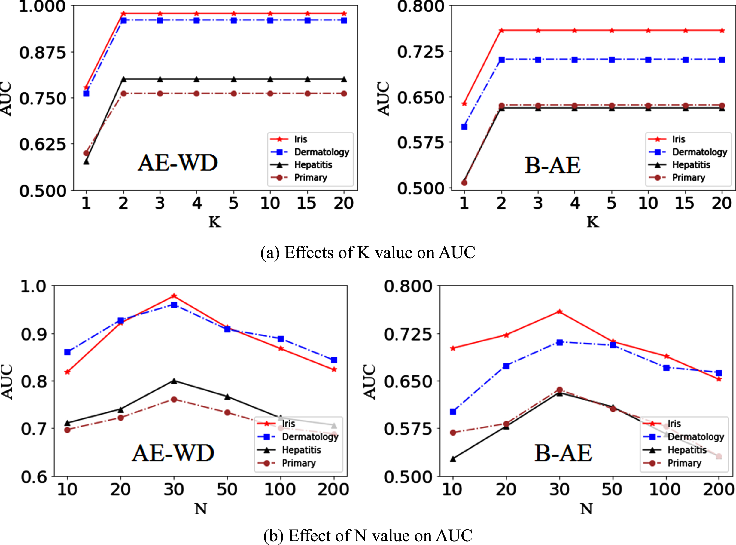
Tested results for K and N value on the benchmark datasets. (a) displays effects of hidden-layer scale on accuracies. (b) displays effects of neuron scale on the accuracies.

4.2 Comparisons of linear separability

The extracted accuracies in Table 2 show that our AE-WD model outperforms competing models and benchmark model on seven datasets, including three benchmark datasets and four high-dimensional datasets. Especially, AE-WD has outstanding advantages on the four high-dimensional dataset Arrhythmia, Madelon, SECOM and ISOLET. However, Competitors m-AE, ISSML, ITML win competitor MMD on most datasets. Figure 2 shows that there are no significant differences between our AE-WD and the competitors. Hence, our AE-WD has outstanding advantages in terms of the extracted accuracy for all considered instances.

Table 2
Extracted accuracies. The best accuracy for each dataset is shown in bold. Distance metric-based models are marked as the symbol +. Feature metric-based models are marked as the symbol = . These models without both metrics are marked as the symbol×

AE-WD (+) m-AE (+) ISSML (+) ITML (+) MMD (=) SAE (×) B-AE (×)

Iris 0.9777±0.0110 0.9744±0.0157 0.9402±0.0154 0.9488±0.0120 0.9247±0.0053 0.9571±0.0227 0.7588±0.3329

Dermatology 0.9602±0.0225 0.9506±0.0137 0.8931±0.0284 0.9374±0.0246 0.7680±0.0377 0.8707±0.0892 0.7112±0.0099

Hepatitis 0.8000±0.1730 0.7703±0.0753 0.7131±0.0642 0.7457±0.0622 0.6897±0.0657 0.6773±0.0373 0.6312±0.1229

Primary 0.7612±0.0709 0.7375±0.0534 0.6886±0.0865 0.6816±0.0745 0.6664±0.0733 0.6700±0.0166 0.6360±0.0002

IDAChallenge 0.6012±0.0019 0.5515±0.0111 0.6666±0.0045 0.6116±0.0135 0.5004±0.0333 0.5166±0.0966 0.5010±0.0099

SCADI 0.6712±0.0551 0.6900±0.0777 0.7116±0.0699 0.6886±0.0004 0.7509±0.0333 0.6666±0.1166 0.6211±0.0100

Arrhythmia 0.7312±0.0222 0.6033±0.0823 0.6188±0.0002 0.6119±0.0444 0.6711±0.0355 0.6999±0.0083 0.5816±0.0187

Madelon 0.6777±0.0266 0.5509±0.0113 0.5600±0.0983 0.5529±0.0009 0.5131±0.0302 0.5679±0.0113 0.4886±0.1227

SECOM 0.6551±0.5333 0.6033±0.3100 0.6100±0.1183 0.5819±0.2229 0.5680±0.1322 0.5229±0.7013 0.4009±0.8997

ISOLET 0.7133±0.6673 0.6337±0.5555 0.6776±0.4448 0.6882±0.0031 0.6000±0.7777 0.6288±0.8113 0.5772±0.1459

	AE-WD (+)	m-AE (+)	ISSML (+)	ITML (+)	MMD (=)	SAE (×)	B-AE (×)
Iris	0.9777±0.0110	0.9744±0.0157	0.9402±0.0154	0.9488±0.0120	0.9247±0.0053	0.9571±0.0227	0.7588±0.3329
Dermatology	0.9602±0.0225	0.9506±0.0137	0.8931±0.0284	0.9374±0.0246	0.7680±0.0377	0.8707±0.0892	0.7112±0.0099
Hepatitis	0.8000±0.1730	0.7703±0.0753	0.7131±0.0642	0.7457±0.0622	0.6897±0.0657	0.6773±0.0373	0.6312±0.1229
Primary	0.7612±0.0709	0.7375±0.0534	0.6886±0.0865	0.6816±0.0745	0.6664±0.0733	0.6700±0.0166	0.6360±0.0002
IDAChallenge	0.6012±0.0019	0.5515±0.0111	0.6666±0.0045	0.6116±0.0135	0.5004±0.0333	0.5166±0.0966	0.5010±0.0099
SCADI	0.6712±0.0551	0.6900±0.0777	0.7116±0.0699	0.6886±0.0004	0.7509±0.0333	0.6666±0.1166	0.6211±0.0100
Arrhythmia	0.7312±0.0222	0.6033±0.0823	0.6188±0.0002	0.6119±0.0444	0.6711±0.0355	0.6999±0.0083	0.5816±0.0187
Madelon	0.6777±0.0266	0.5509±0.0113	0.5600±0.0983	0.5529±0.0009	0.5131±0.0302	0.5679±0.0113	0.4886±0.1227
SECOM	0.6551±0.5333	0.6033±0.3100	0.6100±0.1183	0.5819±0.2229	0.5680±0.1322	0.5229±0.7013	0.4009±0.8997
ISOLET	0.7133±0.6673	0.6337±0.5555	0.6776±0.4448	0.6882±0.0031	0.6000±0.7777	0.6288±0.8113	0.5772±0.1459

Fig. 2

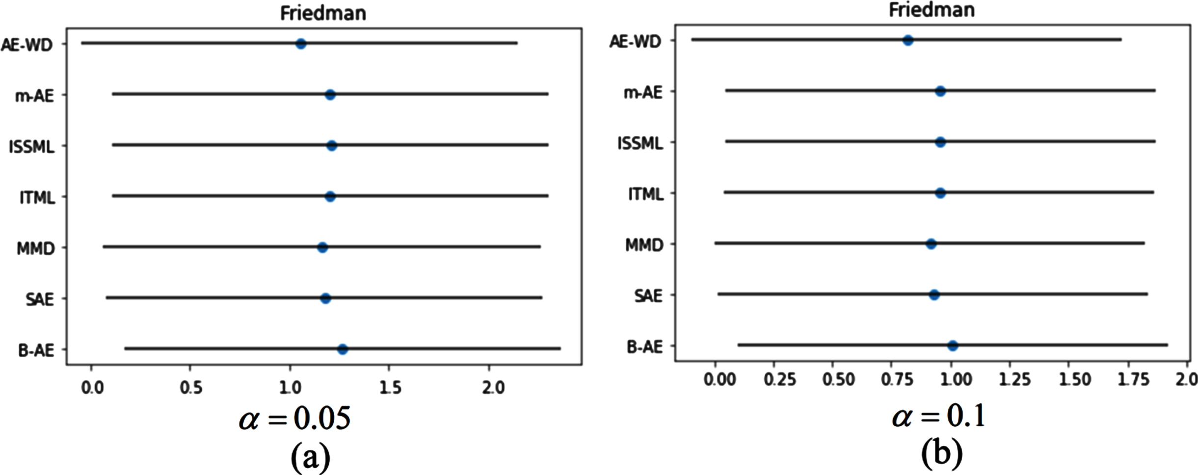
Statistical test results. (a) shows the test results that significance level is equal to 0.05. (b) displays the test results that significance level is equal to 0.1.

To further compare AE-WD with competitors, these extracted features on the four benchmark datasets were projected onto 2-dimensional space using principle component analysis (PCA), and then the projected results were visualized in Fig. 3. The visualized results in Fig. 3 show that it is the best for the margins between different types of features extracted by AE-WD, which means that AE-WD is a winner for the linear separabilities of the extracted features.

Fig. 3

Visualization of the extracted features on the four benchmark datasets. Distance metric-based models are marked as the symbol+. Feature metric-based models are marked as the symbol = . The models without the both metrics are marked as the symbol×. The results of comparison method are cited the [6].

Results on ablation experiments in Fig. 4 indicate that distance metric-based models, e.g., AE-WD m-AE, ISSML and ITML, win over feature metric-based models and deep network architecture-based models in extracted accuracies. Together, these results confirm that distance metric-based models have more outstanding advantages than feature metric-based models and deep network architecture-based models in terms of the linear separabilities of features extraction.

Fig. 4

Results on ablation experiment. Distance metric-based models are marked as the symbol +. Feature metric-based models are marked as the symbol = . The models without the both metrics are marked as the symbol×. (a) displays comparisons between distance metric-based models and the models without the both metrics. (b) displays comparisons of distance metric-based models and feature metric-based models.

4.3 Discussion

The proposed AE-WD gains advantages in feature extraction of linear separabilities, which is because Wasserstein distance in Equation(1) can minimize the difference between the original feature space and the reconstructed feature space. In fact, we performed a homeomorphic transformation on the original feature space, resulting in the so-called reconstructed feature space. Then, in the reconstructed feature space, the autoencoder gains the desired linear separable features, meanwhile, calculating loss function L_f in Equation(6) and using Equation(1) maximizes the classification distance between the extracted different types of features.

Certainly, the proposed AE-WD also has limitations. Due to the extracted ability of AE-WD relies on the reconstructed feature space, Wasserstein distance determines the extracted results for features, i.e., qualities of linear separability. In applications, the calculation of Wasserstein distance is very complex and difficult, so that for large-scale or high-dimensional data, the model might spend more to converge when it is trained, while this does not imply that the model cannot converge.

Distance metric-based methods are evaluated by calculating distance similarity between the data, however, feature metric-based methods are evaluated by obtaining feature importance of the data. Especially, for large-scale or high-dimensional data, the former is more suitable for feature extraction of linear separability than the latter since the calculation of the latter suffers from more difficult. Currently, there are no standard or unified feature importance assessment methods. In addition, autoencoders show excellent capabilities for feature extraction, whereas, they show poorly in feature extraction of linear separability. To address the deficiency, it is recommended that distance metrics are introduced into autoencoders, besides Wasserstein distance metric in the [3] and the [20], also considering Bhattacharyya distance metric in [21].

5 Conclusion

This paper proposes a robust autoencoder with Wasserstein distance for feature extraction of linear separability. Using Wasserstein distance can minimize the difference between the original feature space and the reconstructed feature space. Those features of linearly separability are obtained by using the autoencoder in the reconstructed feature space. Results show that the proposed method wins over the competitors. We demonstrate that the linear separabilities of features obtained by evaluating distance similarity between the data are better than these obtained by evaluating feature importance between the data, and the former is easier to implement than the latter. We also indicate that using the manner of a homeomorphic transformation can reconstruct feature space well, which allows the data distribution in the reconstructed feature space to be closer to the original data distribution. In future work, we will devote more efforts into the feature extraction of linear separability.

Competing interests

The authors declare no conflict of interest.

References

Tao

, Hou

, Nie

et al. Effective Discriminative Feature Selection With Nontrivial Solution[J], IEEE Transactions Neural Network Learning System 27(4) (2016), 796–808.

Luo

, Nie

, Chang

et al. Adaptive Unsupervised Feature Selection With Structure Regularization[J], IEEE Transactions Neural Network Learning System 29(4) (2018), 944–956.

Jian Zheng , Hongchun Qu , Zhaoni Li et al. An irrelevant attributes resistant approach to anomaly detection in high-dimensional space using a deep hyper sphere structure[J], Applied Soft Computing 116 (2022), 1–20.

Ying

, Wen

, Shi

et al. Manifold preserving: An intrinsic approach for semisupervised distance metric learning[J], IEEE Transaction Neural Networks Learning System 29(7) (2018), 2731–2742.

Mei

, Liu

, Karimi

H.R.

et al. Logdet divergence-based metric learning with triplet constraints and its applications[J], IEEE Transaction Image Process 23(11) (2014), 4920–4931.

Jian Zheng , Hongchun Qu , Zhaoni Li et al. A novel autoencoder approach to feature extraction with linear separability for high-dimensional data[J], PeerJ Computer Science 8 (2022), 1–16.

Marco Capo , Aritz Perez and Jose Lozano

, A cheap feature selection approach for the k-means algorithm[J], IEEE Transactions on Neural Networks and Learning Systems 32(5) (2021), 2195–2208.

Ugochukwu Ejike Akpudo , Jang-Wook Hur Intelligent Solenoid Pump Fault Detection based on MFCC Fea-tures, LLE and SVM[C], 2020 International Conference on Artificial Intelligence in Information and Communication (ICAIIC) (2020), 1–3.

Alaor Cervati Neto , Alexandre Levada

L.M.

ISOMAP-KL: a parametric approach for unsupervised metric learning[C], 2020 33rd SIBGRAPI Conference on Graphics, Patterns and Images (SIBGRAPI) (2020), 1–1.

10.

Ang Jun Chin , Andri Mirzal , Habibollah Haron et al. Supervised, Unsupervised and Semi-supervised Feature Selection: A Review on Gene Selection[J], IEEE Transactions on Computational Biology and Bioinformatics 13(5) (2016), 971–989.

11.

Rami Al-Hmouz , Witold Pedrycz , Abdullah Balamash et al. Logic-oriented autoencoders and granular logic autoencoders: developing interpretable data representation[J], IEEE Transactions on Fuzzy Systems 30(3) (2022), 869–877.

12.

Fei Yang , Luis Herranz , Joost van de Weijer et al. Variable rate deep image compression with modulated autoencoder[J], IEEE Signal Processing Letters 27 (2020), 331–335.

13.

Kunjin Chen , Jun Hu , Jinliang He A framework for automatically extracting overvoltage features based on sparse autoencoder[J], IEEE Transactions on Smart Grid 9(2) (2018), 594–604.

14.

Binghao Yan , Guodong Han , Effective feature extraction via stacked sparse autoencoder to improve intrusion detection system[J], IEEE Access 6 (2018), 41238–41248.

15.

Brenier , Yann , Polar factorization and monotone rearrangement of vector-valued functions[J], Commun. Pure Appl. Math 44(4) (1991), 375–417.

16.

Kehua Su , Wei Chen , Na Lei et al. Volume preserving mesh parameterization based on optimal mass transportationation[J], Computer Aided Design 82 (2017), 42–56.

17.

Chen Haodi , Huang Genggeng , Wang Xu-Jia , Convergence rate estimates for aleksandrov’s solution to the monge-ampere equation[J], Siam Journal On Numerical Analysis 57(1) (2019), 173–191.

18.

Na Lei , Kehua Su , Li Cui et al. A geometric view of optimal transportation and generative model[J], Computer Aided Geometric Design 68 (2019), 1–28.

19.

Panaretos , Victor

, Yoav Zemel Statistical aspects of Wasserstein distances[J], Annual Review of Statistics and Its Application (2019), 1–37.

20.

Na Lei , Kehua Su , Li Cui , A geometric view of optimal transportation and generative model[J], Computer Aided Geometric Design 68 (2019), 1–28.

21.

Mariucci

, Reiß

Wasserstein and total vari-ation distance between marginals of Levy processes[J], ArXiv:1710.02715 (2017), 1–1.