Bayesian decision making under soft probabilities

Abstract

Bayesian decision models use probability theory as a commonly technique to handling uncertainty and arise in a variety of important practical applications for estimation and prediction as well as offering decision support. But the deficiencies mainly manifest in the two aspects: First, it is often difficult to avoid subjective judgment in the process of quantization of priori probabilities. Second, applying point-valued probabilities in Bayesian decision making is insufficient to capture non-stochastically stable information. Soft set theory as an emerging mathematical tool for dealing with uncertainty has yielded fruitful results. One of the key concepts involved in the theory named soft probability which is as an immediate measurement over a statistical base can be capable of dealing with various types of stochastic phenomena including not stochastically stable phenomena, has been recently introduced to represent statistical characteristics of a given sample in a more natural and direct manner. Motivated by the work, this paper proposes a hybrid methodology that integrates soft probability and Bayesian decision theory to provide decision support when stochastically stable samples and exact values of probabilities are not available. According to the fact that soft probability is as a special case of interval probability which is mathematically proved in the paper, thus the proposed methodology is thereby consistent with Bayesian decision model with interval probability. In order to demonstrate the proof of concept, the proposed methodology has been applied to a numerical case study regarding medical diagnosis.

Keywords

Soft probability interval probability Bayes rule interval numbers possibility degree

1 Introduction

Bayesian decision making theory has been developed and refined over many decades into a powerful and practical tool. This is due in part to the importance of applications, like economic decisions [1], management science [2], pattern recognition [3] and medical diagnosis [4], that require the rational results of decision making. It is also due to the method with a solid theoretical foundation which facilitates a common-sense interpretation of action and inference under uncertainty. In general, Bayesian decision models consist of two key components, i.e., the Bayes rule and the cost function. Combining the two components, one ends up an associated rule from observations to decision [5]. It is important to note that Bayesian decision models based on traditional probabilities are required to ascertain the subjective probabilities and the related prior distribution using the prior information. But inadequacies lie in that on the one hand it is hardly to estimate point-valued probabilities due to partially known information, especially for non-stochastically stable samples. On the other hand the acquisition of probability assignment frequently depends on subjective judgment which may affect the consistency of the posterior estimations. To overcome the defects, Yager and Kreinovich [6] suggested that due to the large uncertainties in the database a more realistic case of intervally known probabilities instead of exact values can be available, and discussed the decision making techniques in case of interval probabilities. Weichselberger [7] axiomatized the concept of interval probabilities, as well as a discussion on the basic operations, and studied the Bayes rule under the condition of interval probabilities. Guo and Tanaka [8] investigated the newsvendor problem under the decision criteria with interval probabilities. But how to gain the interval-valued probabilities objectively from prior information database is of paramount importance and till now a computational challenge.

Soft set theory [9] was conceived in 1999 as a general mathematical technique to handle with uncertain or imprecise information arising in economics, engineering and environment etc. As the initiator, Molodtsov elaborated his view that the classic uncertain theories such as fuzzy set theory [10], intuitionistic fuzzy set theory [11], rough set theory [12] are sometimes incapable of capturing uncertainties in these domains which present in various types. The reason is possibly the inadequacy of the parametrization tools of these theories. To avoid this drawback, Molodtsov introduced the concept of soft set which uses adequate parametrization such as words and sentences, real numbers, functions, mappings. And explained its advantages for describing uncertainties, as well as providing some potential applications in several directions including game theory, operations research, soft analysis, etc. Later, the same author published a detailed survey of soft set theory [13]. With the formation and development of soft set theory, its applications boom in recent years and have spread to decision making [14 –17], optimization [18], clustering [19], rule mining [20], medical diagnosis [21, 22], systems of soft encryption and decryption [23], assessment [24, 25], etc.

As an important branch of soft set theory, soft probability takes the advantage of adequate parametric tools so as to provide a totally different way of investigating random phenomena with limited samples. It has been successfully applied to some fields like financial portfolio control [26], credit scoring classification [27]. In contrast with the axiomatic definition in the classical probability theory, the main characteristics of soft probability embody that which directly depends on the statistics information and can be seen as an via immediate measurements over the sample base, as well as taking a parametric family of intervals as its values. It is completely data-driven and adapting of not only stochastically stable information but also non-stochastically stable information with small samples. For these reasons, the main aim of this paper is proposed a Bayesian decision model in the framework of soft probability, which can reduce subjectivity in traditional Bayesian decision making and significantly expand the scope of applications.

The remainder of the paper is organized as follows: Section 2 sketches some related background knowledge for preparation. Section 3 presents the method of Bayesian decision making based on soft probabilities, together with the corresponding implement algorithm. A numerical example is employed to illustrate the feasibility and effectiveness of the proposed algorithm in Section 4. Section 5 summarizes several main features of Bayesian risk model with soft probabilities in comparing with the traditional Bayesian decision method. Section 6 concludes the whole paper with a summary and outlook for further research.

2 Preliminaries

2.1 Soft probability

Generally speaking, all phenomena can be divided into three categories. The first one is called deterministic phenomenon with definite regularity. Namely, this kind of phenomenon is under certain conditions, will lead to certain results. Both the second and third categories are classed as the random phenomenon with the condition that results appeared uncertain when facing the certain situations, in which the second one is stochastically stable phenomenon satisfying the large sample statistical laws, the third one as the remaining phenomena existing widely in reality is not stochastically stable that cannot be characterized by classical probability theory.

Soft probability theory initiated by Molodtsov [26] abandons the axiomatic design of classical probability theory and general purposes of calculating the exact probability of the event. Instead, it defines directly over a statistical base, and the value of it is a parametric family of interval numbers, instead of a single point value. As new statistical data appears and the number of sample sequences increases, then these intervals become narrower such that it will be described the phenomenon more accurately. Due to the advantages of without restriction on parametrization tools and totally depending on the investigated sequential samples, soft probability can be capable of handling with any events including not stochastically stable events, in contrast to the classical probability which may be only captured stochastically stable events. Subsequent some basic knowledge regarding soft probability is recalled in brief. Molodtsov [9] first originated the concept of soft set as a new tool to express uncertain information as follows.

Definition 1. [9] Assume that U is an initial universe set of discourse, E is a set of parameters, and let $P (U)$ denote the power set of U. A pair (F, E) is called a soft set over U if and only if F is a mapping given by $F : E \to P (U)$ .

A soft set (F, E) in essence can be interpreted as a parameterized family of subsets of the set U. For each &z.epsi; ∈ E, the set F (&z.epsi;) consists of &z.epsi;-elements or &z.epsi;-approximate elements (solutions, points, etc.). It is worth noting that both Zadeh’s fuzzy set and Pawlak’s rough set can be treated as a special case of soft set, respectively. The notion of soft mapping raised by Molodtsov, as a natural generalization of soft set, is a fundamental tool for constructing soft sets.

Definition 2. [26] Assume that X is a certain set. A pair (F, E) is called a soft mapping over U if and only if F is a mapping from the set of Cartesian product X × E to the power set of U, i.e., $F : X \times E \to P (U)$ .

On the basis of soft mapping, Molodtsov [26] puts forward a new concept of soft probability for dealing with any random events including not stochastically stable events. Suppose that Ω denotes a set of possible outcomes. The outcome of each trial associates with an element of the set Ω. Let R be the set of real numbers. A soft random function denoted by f is any bounded real-valued function over Ω, and the set of f is expressed as $\begin{matrix} F = {f | f : Ω \to R, sup_{ω \in Ω} | f (ω) | < + \infty} . \end{matrix}$ Suppose that as a result of certain repeated q experiments, then one can obtain a sequence of outcomes accordingly, denoted by Base = {ω₁, ω₂, …, ω_q}, where ω_i ∈ Ω. It should be pointed that a statistical base is an ordered set. The cardinality of Base denoted by | Base| = q, and the set of all possible statistical bases denoted by AllBase.

A sample $S_{i}^{k}$ consisting of k elements with statistical starting point ω_i, is a subsequence of the original statistical base given by $\begin{matrix} S_{i}^{k} = (ω_{i}, \dots, ω_{i + k - 1}) . \end{matrix}$ Then the average $〈 f, S_{i}^{k} 〉$ of a soft function f over $S_{i}^{k}$ taken the form of the arithmetic mean, is given by $\begin{matrix} 〈 f, S_{i}^{k} 〉 = \frac{1}{k} \sum_{j = i}^{i + k - 1} f (ω_{j}) . \end{matrix}$ A pair functions $(\underline{μ}, \bar{μ})$ is given by the means of following formulas $\begin{matrix} \underline{μ} (f, Base, k, l) = min_{l \leq i \leq q - k + 1} 〈 f, S_{i}^{k} 〉, \\ \bar{μ} (f, Base, k, l) = max_{l \leq i \leq q - k + 1} 〈 f, S_{i}^{k} 〉 . \end{matrix}$ The two functions $(\underline{μ}, \bar{μ})$ define the left and right endpoints of the average values of a soft random function for a given sample size k from a statistical base starting from a certain number l, respectively. Essentially the pair functions $(\underline{μ}, \bar{μ})$ are soft probability. A formal definition proposed by Molodtsov is given as follows.

Definition 3. [26] A soft mapping (μ, E) over the set of real numbers R is called a soft probability if μ is a mapping $μ : F \times AllBase \times E \to P (R)$ , note that the set of parameters E consists of pairs of natural numbers (k, l), and the mapping μ is given by

$\begin{matrix} μ (f, Base, k, l) = \end{matrix}$ $\begin{matrix} {\begin{matrix} [\underline{μ} (f, Base, k, l), \bar{μ} (f, Base, k, l)] & if k + l \leq | Base | + 1 \\ \emptyset & otherwise \end{matrix} \end{matrix}$

It can be easily seen that soft probability is a parametric family of subintervals of the initial set R. These intervals that determined directly by all sample sizes and all statistical base sizes, provide bounds for the average values of the functions, as well as give a detailed description of average values. With no confusion soft probability is a direct measurement on a statistical base. If the event is stochastically stable, with the increase of sample size, the intervals will tend to be narrow with a large trust degree. If the event is not stochastically stable, with limited sample size, the intervals will be appeared a wide range. And it provides dynamic descriptions of random events when new statistical data appear. These characteristics makes it very convenient to handle with any types of events, including not stochastically stable case.

2.2 Connections between soft probability and interval probability

The main purpose of the current section is to explore connections between soft probability and interval probability. In many instances, the exact values of the probabilities are not easily available due to non-stochastically stable information. Instead, it is customary to employ the intervals of possible values of probabilities. Interval probability adopts an interval number to express the probability measure in order to capture fuzziness and incompleteness in a relatively simple manner.

Definition 4. [7] A triple $F = (Ω, A, P (\cdot))$ consists of a set Ω called the sample space, a σ-field $A$ of random events in Ω, and an interval-valued function $P : A \to 2^{R_{+}}$ . Let P (·) = [L (·) , U (·)], where L (·) and U (·) are the lower bound and the upper bound of P (·), respectively. Then the function P is called an interval probability for which obeys the following axioms:

The interval P (A) = [L (A) , U (A)] ⊆ [0, 1] for $\forall A \in A$

There exists a probability function p (·) satisfying L (A) ≤ p (A) ≤ U (A) for $\forall A \in A$ . Intuitively, for a finite sequence of P₁, P₂, …, P_n, there forms an interval probability distribution if there exist values p₁ ∈ P₁, …, p_n ∈ P_n for which p₁ + … + p_n = 1, i.e., $\sum_{i = 1}^{n} L_{i} \leq 1 \leq \sum_{i = 1}^{n} U_{i}$ .

Let a set of probability functions denoted by $U$ , be called the structure of $F$ with the condition that $U = {p (\cdot) ∣ L (A) \leq p (A) \leq U (A), \forall A \in A}$

If it implies

$\begin{matrix} inf_{p \in U} p (A) = L (A), sup_{p \in U} p (A) \\ = U (A) for \forall A \in A . \end{matrix}$

Note that an interval probability P (A) = [L (A) , U (A)] can be interpreted as a measure of belief, in which L (A) measures the extent to which it is certainly believed that A is true or dependable. 1 - U (A) measures the extent to which it is certainly believed that A is false or undependable. The difference U (A) - L (A) measures the extent of uncertainty of belief in the truth or dependability of A. Five special cases can be derived straightforwardly from the above definition as follows:

$P (\bar{A}) = [1 - U (A), 1 - L (A)]$ indicates the interval probability of the negation of A.

L (∅) =0, U (Ω) =1.

P (A) = [0, 0] indicates a belief that A is certainly false or not dependable.

P (A) = [1, 1] indicates a belief that A is certainly true or dependable.

P (A) = [0, 1] indicates a belief that A is unknown.

For a detailed survey of interval probabilities and their properties, see [7]. The following proposition establishes a connection between internal probability and soft probability.

Proposition 1. Every soft probability can be regarded as an interval probability.

Proof. Let Ω be a sample space, and let Base = {w₁, …, w_q} be a sequence statistical database, w_τ ∈ Ω. Define a sample from the Base consisting of k elements denoted by $S_{t}^{k}$ , satisfying $S_{t}^{k} = (w_{t}, \dots, w_{t + k - 1})$ . Consider a partition of Ω, denoted by {A₁, A₂, …, A_n}, satisfying $⋃_{i = 1}^{n} A_{i} = Ω$ and A_i ⋂ A_j = ∅ (i ≠ j). For an event A_i, the frequency of occurrence of A_i over $S_{t}^{k}$ is given by $\begin{matrix} 〈 χ, S_{t}^{k} 〉 = \frac{1}{k} \sum_{τ = t}^{t + k - 1} χ (ω_{τ}) . \end{matrix}$ Where χ stands for an indicator function of the event A_i, given by $\begin{matrix} χ (A_{i}, ω) = {\begin{matrix} 1 & ω \in A_{i}, \\ 0 & ω \notin A_{i} . \end{matrix} \end{matrix}$ Then the soft probability of A_i is acquired accordingly, denoted by $μ (A_{i}) = [\underline{μ} (A_{i}), \bar{μ} (A_{i})]$ , by using the following formulas $\begin{matrix} \underline{μ} (A_{i}) = min_{t \leq τ \leq q - k + 1} 〈 χ, S_{t}^{k} 〉, \\ \bar{μ} (A_{i}) = max_{t \leq τ \leq q - k + 1} 〈 χ, S_{t}^{k} 〉 . \end{matrix}$ The proofs of axioms I and III are straightforward from the definition of soft probability. For a sequence of soft probabilities $μ (A_{i}) = [\underline{μ} (A_{i}), \bar{μ} (A_{i})] (i = 1, \dots, n)$ , we have $\begin{matrix} \sum_{i = 1}^{n} \underline{μ} (A_{i}) \\ = \underline{μ} (A_{i}) + \sum_{j \neq i} \underline{μ} (A_{j}) \leq \underline{μ} (A_{i}) + \underline{μ} (\cup_{j \neq i} A_{j}) \\ \leq \underline{μ} (A_{i}) + \bar{μ} (\cup_{j \neq i} A_{j}) = 1 . \end{matrix}$ $\begin{matrix} \sum_{i = 1}^{n} \bar{μ} (A_{i}) \\ = \bar{μ} (A_{i}) + \sum_{j \neq i} \bar{μ} (A_{j}) \geq \bar{μ} (A_{i}) + \bar{μ} (\cup_{j \neq i} A_{j}) \\ \geq \bar{μ} (A_{i}) + \underline{μ} (\cup_{j \neq i} A_{j}) = 1 . \end{matrix}$ It implies that axiom II is also established. Thus the proposition is proved that every soft probability can be considered as an interval probability.

2.3 A review of Bayesian decision theory

In current section some fundamental knowledge regarding Bayesian decision theory are recalled for preparation. Informally, a Bayesian decision making is used to select the optimal alternative based on the loss function and the posterior condition probabilities in which the latters are calculated by using Bayes rule on priori probabilities and conditional probabilities. one starts by providing the framework process of the algorithm based on Bayesian decision modeling as the following Fig. 1.

Fig. 1

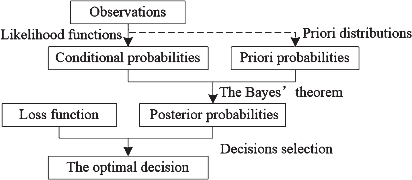
The schematic flow of Bayesian decision making.

Briefly, the Bayesian decision process can be formalized with the help of some related concepts and terminologies. Suppose that D called the decision space, denote the space of all possible decisions d that could be chosen by a decision maker (abbreviated as DM), let Θ be the space of all possible states of nature θ. Assign λ to a function called loss function, where λ (d, θ) represents loss quantity when the DM adopts decision d under the specific state θ. For simplicity assume that D = {d₁, …, d_m} and Θ = {θ₁, …, θ_n} are finite of respective dimensions m and n. Thereby eventually the losses {λ (d_i, θ_j) = λ_ij|i = 1, … , m ; j = 1, …, n } can be constructed a m × n matrix form called the decision-loss table that can be expressed as below.

$\begin{matrix} [λ (d_{i}, θ_{j})] \\ = (\begin{matrix} θ_{1} & θ_{2} & \dots & θ_{n} \\ d_{1} & λ (d_{1}, θ_{1}) & λ (d_{1}, θ_{2}) & \dots & λ (d_{1}, θ_{n}) \\ d_{2} & λ (d_{2}, θ_{1}) & λ (d_{2}, θ_{2}) & \dots & λ (d_{2}, θ_{n}) \\ ⋮ & ⋮ & ⋮ & ⋮ & ⋮ \\ d_{m} & λ (d_{m}, θ_{1}) & λ (d_{m}, θ_{2}) & \dots & λ (d_{m}, θ_{n}) \end{matrix}) . \end{matrix}$

The Bayesian modeling framework for choosing a good decision is to pick a decision whose associated expected loss to the DM is minimized. Let X be a vector called the feature vector in which entries are the observation values that describing the states in Θ. With a given trial, the DM obtains a concrete observation X. Given the priori probability of each state θ_j written by P (θ_j) and the conditional probability of X given θ_j written by P (X|θ_j), then the posterior probability is calculated by using Bayes’ rule

$\begin{matrix} P (θ_{j} | X) = \frac{P (X | θ_{j}) P (θ_{j})}{P (X)} . \end{matrix}$

Where P (X) is computed by applying the law of total probability

$\begin{matrix} P (X) = \sum_{j = 1}^{n} P (X | θ_{j}) P (θ_{j}) . \end{matrix}$

With regard to a certain feature vector X, then the Bayes risk of choosing decision d_i denoted by R (d_i| X) is the expected loss value of λ (d_i, θ_j) with respect to the posterior distribution derived by the following style

$\begin{matrix} R (d_{i} | X) = E [λ (d_{i}, θ_{j})] = \sum_{j = 1}^{n} λ (d_{i}, θ_{j}) P (θ_{j} | X) . \end{matrix}$

The smaller risk value R (d_i| X), the better alternative d_i will be. A decision d^∗ ∈ D which minimizes R (d_i| X) is called a Bayes decision.

The algorithm of Bayesian decision making consists of several typical steps introduced as below:

Step 1: Address the set of initial states and the set of decisions.

Step 2: Prepare decision-loss table [λ (d_i, θ_j)] as follows

$\begin{matrix} [λ (d_{i}, θ_{j})] = (\begin{matrix} θ_{1} & θ_{2} & \dots & θ_{n} \\ d_{1} & λ_{11} & λ_{12} & \dots & λ_{1 n} \\ d_{2} & λ_{21} & λ_{22} & \dots & λ_{2 n} \\ ⋮ & ⋮ & ⋮ & ⋮ & ⋮ \\ d_{m} & λ_{m 1} & λ_{m 2} & \dots & λ_{mn} \end{matrix}) . \end{matrix}$

Step 3: Given a certain feature vector X, according to the priori probability P (θ_j) and the conditional probability θ_j given X denoted by P (X|θ_j), calculate the posterior probability P (θ_j|X)

$\begin{matrix} P (θ_{j} | X) = \frac{P (X | θ_{j}) P (θ_{j})}{\sum_{j = 1}^{n} P (X | θ_{j}) P (θ_{j})}, \\ j = 1, 2, \dots, n . \end{matrix}$

Step 4: In accordance with the posterior probability P (θ_j|X) and decision-loss matrix [λ (d_i, θ_j)], the Bayes risk by taking d_i denoted by R (d_i| X) is formulated as $\begin{matrix} R (d_{i} | X) = \sum_{j = 1}^{n} λ (d_{i}, θ_{j}) P (θ_{j} | X) . \end{matrix}$ Step 5: Rank all decisions based on the values of the Bayes risk R (d_i| X), Bayesian decision rule selects the decision d^∗ that minimizes R (d_i| X) (i = 1, 2, …, m) and is the best target could do $\begin{matrix} d^{*} = arg min_{d_{i}} R (d_{i} | X) . \end{matrix}$ For a more detailed discussion of Bayesian decision theory, one can refer to [28].

3 Bayesian decision model with soft probabilities

Our goal in this section is to rigorously integrate with soft probability and Bayesian decision rule, to present the methodology with which to copy with multiple attribute decision making where the input arguments are interval values instead of possible point values. The proposed model has the characteristics of soft probability and Bayes risk, and it is therefore named as soft probability based Bayes risk model. It is worth noting that they are natural generalizations of the method of risk-minimum Bayesian decision.

Consider a typical multiple attribute decision making problem, which contains m decision alternatives d_i, i = 1, 2, …, m and n states θ_j, j = 1, 2, …, n. Let X₁, …, X_s be a set of attributes or features. Assign a feature vector X to be a complete assignation of attributes for depicting each state, denoted by X = x, where x = {X₁ = x₁, …, X_s = x_s}, i.e., a vector x is uniquely corresponding to a certain state θ ∈ Θ. In addition, these states evaluate the alternatives by using of decision-loss matrix [λ (d_i, θ_j)], where λ (d_i, θ_j) represents the value loss of of adopting alternative d_i when meets with real state θ_j that determines in advance. Note that the priori probability P (θ_j) and the conditional probability P (X|θ_j) are soft probabilities which are expressed by real subintervals of [0, 1]. The main goal is to choose the optimal decision with minimum Bayes risk. Subsequent the detailed procedure of the proposed method is illustrated as the following steps.

3.1 Calculating conditional soft probabilities

In Bayesian theory, the conditional probabilities are assumed as known point values. But when the problem is modeled by soft probabilities, not all the conditional probabilities are need to be known in advance. It is possible to approximate the unknown conditional probabilities by applying the definition of soft probability and historical bases with priori information.

Given the priori information that there exists a series of historical data {x_tj } (t = 1, 2, …, T) for each attribute X_η (η = 1, 2, …, s) and {θ_t} (t = 1, 2, …, T) for taking value in the states space Θ = {θ₁, θ₂, …, θ_s}, respectively. Where x_tj is a binary value of 1 or 0 with respect to attribute X_j at time t, namely meets or not meets the attribute X_j. In what follows a historic database denoted by Base^T = (Base₁, Base₂, …, Base_T) consists of T records Base_t, each contains basic data with regard to the ${Base}_{t} = ({Data}_{X_{1}}^{t}, {Data}_{X_{2}}^{t}, \dots, {Data}_{X_{s}}^{t}, {Data}_{Θ}^{t}) = (x_{t 1}, x_{t 2}, \dots, x_{ts}, {Data}_{Θ}^{t})$ , where ${Data}_{Θ}^{t}$ is a specific state θ in the state space Θ at time t.

Given a state θ_j ∈ Θ, one can define an indicator function χ as follows $\begin{matrix} χ_{j}^{t} = {\begin{matrix} 1 & θ_{t} = θ_{j}, \\ 0 & θ_{t} \neq θ_{j} . \end{matrix} \end{matrix}$ By using of the aforementioned strategy, a multi-class classification for decision space can be reduced to a multiple (n) binary classifications.

Therefore, one can obtain the basic data related to decision making consists of attributes and states denoted by ${Base}_{t} = (x_{t 1}, x_{t 2}, \dots, x_{ts}, χ_{j}^{t}), t \in {1, 2, \dots, T}, j \in {1, 2, \dots, n}$ . Let I ={ (k, l) }, one typically take l = 1 [29], and k is acquired differently in the terms of different backgrounds. According to Definition 3, we naturally construct a mapping μ : F × Allbase × I → E, denoted by μ (f, Base^T, k, l). Thus one can obtain the soft probability $[{\underline{μ}}_{j}, {\bar{μ}}_{j}]$ of the state {Θ = θ_j}. And the conditional soft probability of {X_η = x_η} given Θ_j = θ_j denoted by $[\underline{μ} (X_{η} = x_{η} | Θ = θ_{j}), \bar{μ} (X_{η} = x_{η} | Θ = θ_{j})]$ can be derived in a similar way.

3.2 Ascertaining joints and posterior soft probabilities

Let X = (X₁, X₂, …, X_s) be independent, jointly distributed random vectors by assuming independence among attributes, i.e., under the Naive Bayes assumption, the joint soft probabilities of attributes {X_η = x_η| Θ = θ_j} (η = 1, 2, …, s) are calculated as follows $\begin{matrix} \underline{μ} (X = x | Θ \\ = θ_{j}) = \underline{μ} (X_{1} = x_{1}, \dots, X_{s} = x_{s} | Θ = θ_{j}) \\ = Π_{η = 1}^{s} \underline{μ} (X_{η} = x_{η} | Θ = θ_{j}), \end{matrix}$ $\begin{matrix} \bar{μ} (X = x | Θ = θ_{j}) \\ = \bar{μ} (X_{1} = x_{1}, \dots, X_{s} = x_{s} | Θ = θ_{j}) \\ = Π_{η = 1}^{s} \bar{μ} (X_{η} = x_{η} | Θ = θ_{j}) . \end{matrix}$ Due to the fact that both the priori soft probabilities and the joint soft probabilities of conditional attributes can be seen as special cases of interval probabilities. By using Bayesian formula with interval probabilities [7], the posterior soft probabilities are formulated as follows $\begin{matrix} \underline{μ} (Θ = θ_{j} | X = x) = \end{matrix}$ $\begin{matrix} \frac{\underline{μ} (X = x | Θ = θ_{j}) {\underline{μ}}_{j}}{\underline{μ} (X = x | Θ = θ_{j}) {\underline{μ}}_{j} + \sum_{t \neq j} \bar{μ} (X = x | Θ = θ_{t}) {\bar{μ}}_{t}}, \end{matrix}$

$\begin{matrix} \bar{μ} (Θ = θ_{j} | X = x) = \end{matrix}$ $\begin{matrix} \frac{\bar{μ} (X = x | Θ = θ_{j}) {\bar{μ}}_{j}}{\bar{μ} (X = x | Θ = θ_{j}) {\bar{μ}}_{j} + \sum_{t \neq j} \underline{μ} (X = x | Θ = θ_{t}) {\underline{μ}}_{t}} . \end{matrix}$

3.3 Bayes risk minimization

Bayesian decision making associates a loss function λ (d_i, θ_j) to measure the loss of classifying the alternative θ_t to class θ_j. Given the feature vector X = x and the loss function λ (d_i, θ_j), then the Bayes risk of adopting alternative d_i with respect to x is defined as $\begin{matrix} R (d_{i} | x) = [\underline{R} (d_{i} | x), \bar{R} (d_{i} | x)] . \end{matrix}$ Where $\begin{matrix} \underline{R} (d_{i} | x) = \sum_{j = 1}^{n} λ (d_{i}, θ_{j}) \underline{μ} (Θ = θ_{j} | X = x), \\ \bar{R} (d_{i} | x) = \sum_{j = 1}^{n} λ (d_{i}, θ_{j}) \bar{μ} (Θ = θ_{j} | X = x) . \end{matrix}$ It is critical to note that the above Bayes risk R (d_i|x) is in the form of interval number. Therefore, taking into account the situation one would have to consider comparison of Bayes risk on the basis of the ranking principle of interval numbers [30], which can be depicted as follows. Let interval numbers a = [a_L, a_U] and b = [b_L, b_U] be given, and let S (a) = a_U - a_L, S (b) = b_U - b_L. The possible degree for interval number ranking is given by $\begin{matrix} p (a \geq b) = \frac{min {S (a) + S (b), max (a_{U} - b_{L}, 0)}}{S (a) + S (b)} . \end{matrix}$ Where p (a ≥ b) measures the possible degree of a is superiority, equivalent and inferiority than b. By definition, the possible degree satisfies p (a ≥ b) ∈ [0, 1], one needs to calculate the possible degree p (a ≥ b) to which a dominates b. It is worth noting that p (a ≥ b) > 1/2, p (a ≥ b) = 1/2, p (a ≥ b) < 1/2 implies a > b, a = b, a < b respectively. The following properties are obviously established.

Proposition 2. Let a = [a_L, a_U] , b = [b_L, b_U] , c = [c_L, c_U] be three interval numbers.

p (a ≥ b) + p (b ≥ a) =1;

If p (a ≥ b) = p (b ≥ a), then p (a ≥ b) = p (b ≥ a) =1/2;

If a_U ≤ b_L, then p (a ≥ b) =0, if b_U ≤ a_L, then p (a ≥ b) =1;

If p (a ≥ b) ≥1/2 and p (b ≥ c) ≥1/2, then p (a ≥ c) ≥1/2.

Proof. (1) For a_U ≥ b_L, according the definition of possible degree, we can write $\begin{matrix} p (a \geq b) + p (b \geq a) \\ = \frac{min {S (a) + S (b), max (a_{U} - b_{L}, 0)}}{S (a) + S (b)} \\ + \frac{min {S (a) + S (b), max (b_{U} - a_{L}, 0)}}{S (a) + S (b)} . \end{matrix}$ If b_U ≤ a_L, then a_U - b_L ≥ a_U - a_L + b_U - b_L = S (a) + S (b), one can obtain $\begin{matrix} p (a \geq b) + p (b \geq a) = \frac{S (a) + S (b)}{S (a) + S (b)} + 0 = 1 . \end{matrix}$ If b_U > a_L, then a_U - b_L < a_U - a_L + b_U - b_L = S (a) + S (b), one can obtain $\begin{matrix} p (a \geq b) + p (b \geq a) \\ = \frac{a_{U} - b_{L}}{S (a) + S (b)} + \frac{b_{U} - a_{L}}{S (a) + S (b)} \\ = \frac{(a_{U} - a_{L}) + (b_{U} - a_{L})}{S (a) + S (b)} = \frac{S (a) + S (b)}{S (a) + S (b)} = 1 . \end{matrix}$ Similarly, for a_U < b_L, b_U - a_L > b_U - b_L + a_U - a_L = S (b) + S (a), one can obtain $\begin{matrix} p (a \geq b) + p (b \geq a) = 0 + \frac{S (a) + S (b)}{S (a) + S (b)} = 1 . \end{matrix}$ This completes the proof.

(2) It can be straightforward obtained according to (1).

(3) If a_U ≤ b_L, due to the fact that S (a) + S (b) = a_U - a_L + b_U - b_L ≥ 0, then $\begin{matrix} p (a \geq b) = \frac{min {S (a) + S (b), max (a_{U} - b_{L}, 0)}}{S (a) + S (b)} \\ = \frac{0}{S (a) + S (b)} = 0 . \end{matrix}$ If b_U ≤ a_L, then a_U - b_L ≥ a_U - a_L + b_U - b_L = S (a) + S (b). Therefore $\begin{matrix} p (a \geq b) = \frac{min {S (a) + S (b), max (a_{U} - b_{L}, 0)}}{S (a) + S (b)} \\ = \frac{S (a) + S (b)}{S (a) + S (b)} = 1 . \end{matrix}$

(4) It is easily proved that the equivalent form for p (a ≥ b) ≥1/2 is satisfying a_U + a_L ≥ b_U + b_L. At the same reason, the equivalent form for p (b ≥ c) ≥1/2 is satisfying b_U + b_L ≥ c_U + c_L. Consequently, a_U + a_L ≥ c_U + c_L, hence it can be concluded that p (a ≥ c) ≥1/2. This completes the proof.

Thus, we can compare Bayes risk under different decision by means of possible degrees of interval numbers. The possible degree of the pairwise comparisons judgment matrix is therefore established as follows $\begin{matrix} P = [p_{ij}]_{m \times m} = {[p (R (d_{i} | x) \geq R (d_{j} | x))]}_{m \times m} . \end{matrix}$ Without lose of generality, if p_ij ≥ 1/2, then the alternative d_j dominates d_i due to the reason of smaller Bayes risk. According to the matrix P, one can rank all these alternatives and select the most desirable one(s).

Take d_{j
^∗} ∈ {d₁, d₂, …, d_m} such that p_{ij
^∗} ≥ 1/2 for ∀d_i ∈ {d₁, d₂, …, d_m}. Equivalently, it satisfies the form $\begin{matrix} min_{i \in {1, 2, \dots, m}} p_{{ij}^{*}} = p_{j^{*} j^{*}} = \frac{1}{2} . \end{matrix}$ It is straightforward to verify that the above-mentioned formula implies d_{j
^∗} is the optimal decision which minimizes Bayes risk. The implement algorithm of Bayesian decision making under soft probabilities is illustrated as follows.

Step 1: Input the set of decision alternatives D = {d₁, d₂, …, d_m} and a finite state space Θ = {θ₁, θ₂, …, θ_n}, as well as a set of attributes X = {X₁, X₂, …, X_s} for characterizing each state;

Step 2: Quantify the consequences of choosing each decision d_i ∈ D for each possible outcome θ_j ∈ Θ. Namely derive the losses {λ (d_i, θ_j) = λ_ij} (i = 1, 2, …, m, j = 1, 2, …, n) which can be specified as an m × n decision-loss matrix [λ_ij] _mn

Step 3: With the help of the states data of the time series and attributes data with respect to each state contained in the priori information, one establishes a historic database Base^T = (Base₁, Base₂, …, Base_T). Assign the statistical starting point l and the size of sample k, denote the pair E = (l, k);

Step 4: Construct the soft mapping (μ, E) according to Definition 3, where μ is a pair functional denoted by $μ = [\underline{μ}, \bar{μ}]$ , thus calculate the priori soft probability $[{\underline{μ}}_{j}, {\bar{μ}}_{j}]$ and the conditional soft probability of each state (j = 1, 2, …, n ; η = 1, 2, …, s) as follows $\begin{matrix} [\underline{μ} (X_{η} = x_{η} | Θ = θ_{j}), \bar{μ} (X_{η} = x_{η} | Θ = θ_{j})]; \end{matrix}$ Step 5: Given an attributes vector x, derive the joint soft probabilities of attributes given state Θ = θ_j, denoted by $[\underline{μ} (X = x | Θ = θ_{j}), \bar{μ} (X = x | Θ = θ_{j})]$ . According to Bayes Rule under interval probabilities, thus compute the posterior soft probabilities $[\underline{μ} (Θ = θ_{j} | X = x), \bar{μ} (Θ = θ_{j} | X = x)]$

Step 6: Measure the Bayes risk associated with each d_i, denoted by R (d_i|x) (i = 1, 2, …, m). By using of interval number ranking principle, rank all decision alternatives and select the optimal decision by minimizing the Bayes risk.

The flowchart of the algorithm above is shown in Fig. 2 as follows.

Fig. 2

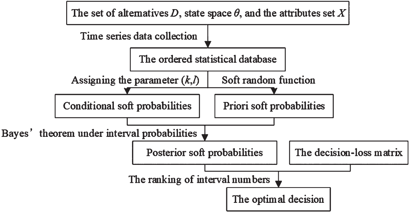
The flowchart of Bayesian decision making with soft probabilities.

4 Illustrative example

In order to test validity and effectiveness of the proposed method, an illustrative example is given as follows.

Generally in medical diagnosis a patient suffering from a disease may have multiple visible symptoms. And it is also important to note that there exists certain symptoms which may be in common to more than one disease leading to diagnostic dilemma. Doctors always detect clinical manifestations based on analysis of historical diagnosis information to find the most probable disease. In addition, the possibilities of misdiagnosis exist in same cases, and wrong judgement usually leads to different consequences or losses. As a consequence, it can be formulated as a Bayesian decision problem, and the above proposed approach brings much convenience to deal with the existing uncertainty in the process of medical diagnosis.

Now consider a medical diagnosis problem with four symptoms such as headache, chest pain, cough and fever which have more or less contribution in two diseases such as flu or pneumonia. Here denotes the set of attributes as X = {x₁ =“headache”,x₂ =“chest pain”,x₃ =“cough”,x₄ =“fever”}, and denotes the set of states as Θ = {θ₁=F, θ₂=P}. For simplicity here F and P represent flu and pneumonia, respectively. There already exist ten patients {u₁, u₂, …, u₁₀} which were diagnosed successively and thus a cases statistical base was established as shown in Table 1.

Table 1
The tabular representation of cases statistical base

Patient x₁ =“headache” x₂ =“chest pain” x₃ =“cough” x₄ =“fever” Θ={flu,pneumonia}

u ₁ 1 1 1 1 P

u ₂ 1 1 0 1 F

u ₃ 1 0 1 0 F

u ₄ 0 1 1 1 P

u ₅ 1 0 1 0 F

u ₆ 0 1 0 1 F

u ₇ 1 0 0 0 F

u ₈ 1 1 1 1 F

u ₉ 1 1 0 1 P

u ₁₀ 0 0 1 1 P

Patient	x₁ =“headache”	x₂ =“chest pain”	x₃ =“cough”	x₄ =“fever”	Θ={flu,pneumonia}
u ₁	1	1	1	1	P
u ₂	1	1	0	1	F
u ₃	1	0	1	0	F
u ₄	0	1	1	1	P
u ₅	1	0	1	0	F
u ₆	0	1	0	1	F
u ₇	1	0	0	0	F
u ₈	1	1	1	1	F
u ₉	1	1	0	1	P
u ₁₀	0	0	1	1	P

In Table 1, if a patient u_t has a symptom x_η, then x_tη = 1, else x_tη = 0.

Suppose a new patient u₁₁ who is suffering a disease that has the symptoms consisting of headache, cough and fever. Now the problem is how a doctor detects the actual disease with the priori knowledge on the basis of cases statistical base and the exhibited symptoms among the two diseases for that patient. Apply the proposed method to detect which disease that is most consistent with symptoms. The investigative procedures are addressed as follows.

Step 1: In the decision making, we consider the two classes of diagnostic decisions, i.e., diagnose the illness as flu (abbre. d_f) or diagnose the illness as pneumonia (abbre. d_p), these two categories constitute a decision space denoted by D = {d_f, d_p}. We consider the set of states Θ = {θ₁=F,θ₂=P} as a state space and the set of attributes which contains a diagnosis parameter system, denoted by X = {x₁ =“headache”, x₂ =“chest pain”, x₃ =“cough”, x₄ =“fever”}.

Step 2: Determine the loss function λ (d_i, θ_j) that measures the loss of classifying patient u_t into class d_i knowing that the state is θ_j. It is worthwhile to note that different loss function will yield different decision loss. Due to the fact that “0-1” model is the commonly used loss function, and it can effectively assess the correctness of decision making. Therefore, with the aid of “0-1” model, the decision-loss matrix [λ (d_i, θ_j)] (i = 1, 2 ; j = 1, 2) is expressed as follows $\begin{matrix} = (\begin{matrix} θ_{1} = F & θ_{2} = P \\ d_{f} & 0 & 1 \\ d_{p} & 1 & 0 \end{matrix}) . \end{matrix}$ 3: As a result of the sequence of diagnostic cases, a statistical base is thus formed, denoted by Base^T = (Base₁, Base₂, …, Base_T), where T denotes the case numbers, i.e., T = 10. And ${Base}_{t} = (x_{t 1}, x_{t 2}, \dots, x_{ts}, χ_{j}^{t})$ , in which $χ_{j}^{t}$ denotes the patient u_t is suffering θ_j (θ_j ∈ Θ = {θ₁ =F, θ₂=P}). We denote a pair E = (l, k), where l indicates the statistical starting point and is set to 1, k indicates the size of sample and is set to 3;

Step 4: Construct a soft mapping (μ, E) by Definition 3, thereby the priori soft probability of suffering flu and suffering pneumonia are calculated respectively as follows

$\begin{matrix} μ (θ_{j} = F) = [\underline{μ} (θ_{j} = F), \bar{μ} (θ_{j} = F)] . \end{matrix}$ Where $\begin{matrix} \underline{μ} (θ_{j} = F) = min_{1 \leq i \leq 8} \frac{1}{3} \sum_{j = i}^{i + 2} χ (F, θ_{j}) = \frac{1}{3}, \\ \bar{μ} (θ_{j} = F) = max_{1 \leq i \leq 8} \frac{1}{3} \sum_{j = i}^{i + 2} χ (F, θ_{j}) = 1 . \end{matrix}$ And $\begin{matrix} μ (θ_{j} = P) = [\underline{μ} (θ_{j} = P), \bar{μ} (θ_{j} = P)] . \end{matrix}$ Where $\begin{matrix} \underline{μ} (θ_{j} = P) = min_{1 \leq i \leq 8} \frac{1}{3} \sum_{j = i}^{i + 2} χ (P, θ_{j}) = 0, \\ \bar{μ} (θ_{j} = P) = max_{1 \leq i \leq 8} \frac{1}{3} \sum_{j = i}^{i + 2} χ (P, θ_{j}) = \frac{2}{3} . \end{matrix}$ The results of conditional soft probability with regard to suffering flu or pneumonia are calculated respectively in a similar way and showed in the following Table 2.

Table 2

The conditional soft probability with respect to flu or pneumonia

$μ (x_{1} = 1 \| θ_{1} = F) = [\frac{2}{3}, 1]$	$μ (x_{1} = 0 \| θ_{1} = F) = [0, \frac{1}{3}]$	$μ (x_{2} = 1 \| θ_{1} = F) = [\frac{1}{3}, \frac{2}{3}]$	$μ (x_{2} = 0 \| θ_{1} = F) = [\frac{1}{3}, \frac{2}{3}]$
$μ (x_{1} = 1 \| θ_{2} = P) = [\frac{1}{3}, \frac{2}{3}]$	$μ (x_{1} = 0 \| θ_{2} = P) = [\frac{1}{3}, \frac{2}{3}]$	$μ (x_{2} = 1 \| θ_{2} = P) = [\frac{2}{3}, 1]$	$μ (x_{2} = 0 \| θ_{2} = P) = [0, \frac{1}{3}]$
$μ (x_{3} = 1 \| θ_{1} = F) = [\frac{1}{3}, \frac{2}{3}]$	$μ (x_{3} = 0 \| θ_{1} = F) = [\frac{1}{3}, \frac{2}{3}]$	$μ (x_{4} = 1 \| θ_{1} = F) = [\frac{1}{3}, \frac{2}{3}]$	$μ (x_{4} = 0 \| θ_{1} = F) = [\frac{1}{3}, \frac{2}{3}]$
$μ (x_{3} = 1 \| θ_{2} = P) = [\frac{2}{3}, 1]$	$μ (x_{3} = 0 \| θ_{2} = P) = [0, \frac{1}{3}]$	μ (x₄ = 1\|θ₂ = P) = [1, 1]	μ (x₄ = 0\|θ₂ = P) = [0, 0]

Step 5: Given the new patient u₁₁ with observed symptoms of headache, cough and fever, written by x^∗ = (x₁ = 1, x₂ = 0, x₃ = 1, x₄ = 1). In order to obtain the posterior soft probabilities, a straightforward computation of joint soft probabilities of attributes based on the attribute independence assumption shows that

$\begin{matrix} [\underline{μ} (x = x^{*} | θ_{1} = F), \bar{μ} (x = x^{*} | θ_{1} = F)] \\ = [\frac{2}{3^{5}}, \frac{8}{3^{3}}], \\ [\underline{μ} (x = x^{*} | θ_{2} = P), \bar{μ} (x = x^{*} | θ_{2} = P)] \\ = [0, \frac{4}{3^{3}}] . \end{matrix}$ Therefore the posterior soft probabilities are calculated by utilizing Bayes Rule as follows $\begin{matrix} [\underline{μ} (θ_{1} = F | x = x^{*}), \bar{μ} (θ_{1} = F | x = x^{*})] \\ = [\frac{1}{19}, 1], \\ [\underline{μ} (θ_{1} = P | x = x^{*}), \bar{μ} (θ_{2} = P | x = x^{*})] \\ = [0, \frac{18}{19}] . \end{matrix}$ Step 6: It follows that the Bayes risks of the two decisions given the exhibit symptom are given by $\begin{matrix} R (d_{1} | x^{*}) = R (d = d_{f} | x = x^{*}) \\ = \sum_{j = 1}^{2} λ_{1 j} μ (θ_{j} | x^{*}) = [0, \frac{18}{19}], \\ R (d_{2} | x^{*}) = R (d = d_{p} | x = x^{*}) \\ = \sum_{j = 1}^{2} λ_{2 j} μ (θ_{j} | x^{*}) = [\frac{1}{19}, 1] . \end{matrix}$ From the possible degree for interval number ranking, a minimizer of R (d_i|x^∗) with respect to d_i is determined as follows $\begin{matrix} p (R (d_{1} | x^{*}) \geq R (d_{2} | x^{*})) \approx 0.42 < 0.5 . \end{matrix}$ Hence R (d₁|x^∗) < R (d₂|x^∗). In this case, the doctor prefers d₁ = d_f to d₂ = d_p, i.e., the Bayes decision is d_f that the patient u₁₁ should be diagnosed as flu with the exhibited symptom x^∗

Increasing the initial statistical scale l would effectively reduce the interval width of priori soft probability and make the results of decisions more accurate. For instance, let l = 4, one can obtain $μ (θ_{1} = F) = [\frac{1}{2}, 1], μ (θ_{2} = P) = [0, \frac{1}{2}]$ . Perform the same procedures repeatedly, one can get the following results $\begin{matrix} R (d_{1} | x^{*}) = R (d = d_{f} | x = x^{*}) = [0, \frac{2}{3}], \\ R (d_{2} | x^{*}) = R (d = d_{p} | x = x^{*}) = [\frac{1}{3}, 1] . \end{matrix}$ The results guarantee that p (R (d₁|x^∗) ≥ R (d₂|x^∗)) ≈ 0.33 < 0.5. By the same token, R (d₁|x^∗) < R (d₂|x^∗), thus u₁₁ is also diagnosed as flu that is completely consistent with the previous conclusion, and as we can seen the possibility of being diagnosed with flu is further enhanced.

Be noted that, in the example above, the patients u₂ and u₉ exhibit exactly the same symptoms with total different diagnosis results. Actually such situation is very common in medical diagnosis problems due to the fact that certain common symptoms may be linked to more than one disease. In this case, it is necessary to evaluating the possibility of suffering from alternative diseases on the basis of historical statistical database. Take into account the new patient u₁₁ who is suffering a disease that has the same symptoms with patients u₂ and u₉. In the same respect, let k = 1, l = 4, by applying the algorithm above one will have

$\begin{matrix} R (d_{1} | x^{*}) = R (d = d_{f} | x = x^{*}) = [0, \frac{4}{5}], \\ R (d_{2} | x^{*}) = R (d = d_{p} | x = x^{*}) = [\frac{1}{5}, 1] . \end{matrix}$

The ranking of interval Bayesian risk is calculated as follows: p (R (d₁|x^∗) ≥ R (d₂|x^∗)) = 0.375 < 0.5, i.e. R (d₁|x^∗) < R (d₂|x^∗). That means u₁₁ should be diagnosed as flu based on the available information. The essential reason for this result is that priori soft probability $μ (θ_{1} = F) = [\frac{1}{2}, 1]$ is superiority than $μ (θ_{2} = P) = [0, \frac{1}{2}]$ . Therefore the new patient u₁₁ is more likely suffering from flu.

It worth noting that the historical statistical database only contains 10 samples in this illustration. The limited sample size may, to some extent, has restricted the results obtained by using Bayesian risk model with soft probabilities, causing the diagnosis accuracy is naturally not high. However, with the increase of the sample size, the interval values of soft probabilities will become narrower. As a result, the accuracy of diagnostic results will graduallyincrease.

5 Discussion

Note that the proposed method integrates soft probabilities and the traditional Bayes risk model. The interval value of soft probability could be obtained automatically based on soft random function, and it has the ability of dealing with not stochastically stable information with limited samples. In comparing Bayes risk model, the proposed model typically has the advantage of less restrictions and wider application scenarios but the disadvantage of being more difficult to understand and compute. The key features of the proposed model can be concluded asfollows:

Unlike classical Bayes risk model, in which the priori probability is calculated based on prior distribution, or subjective experience, and is only applicable to stochastically stable phenomena. The proposed model does not require prior distribution information, and the priori soft probability can be seen as an objective probability that is directly relying on the statistical base and completely data driven. This makes it a more adequate formalism for application scenarios where the information is stochastically stable or not stochastically stable, and there is no limit on the samplesize.

The results of Bayesian decision can be dynamic adjusted when new statistical data appear. The soft probability will be a sufficiently narrow interval if the sample size is large enough. This leads to a more accurate posterior probability, thus the performance of Bayesian decision with soft probabilities performs more accurate with the increase in the amount of samples. Meanwhile, the formalism of the corresponding algorithm can be implemented easily in practice.

Soft probability takes a subinterval of [0, 1] as its value, it satisfies the axiomatic definition of interval probability, and can be seen as a special form of interval probability. Therefore, Bayesian decision model with soft probabilities is naturally compatible with the mature Bayesian decision model with interval probabilities. Furthermore, due to the fact that soft probability gives a detailed description of bounds for the average values for all sample sizes and all statistical base sizes, which makes Bayesian decision under soft probability is more suitable for dealing with the actual situations, especially not stochastically stable phenomena.

6 Concluding remarks

Decision making coping with practical problems is often under the condition of time series data that requires extraction of the statistical regulation from a set of samples regarding alternatives and their characteristics. These assessments are generally performed with uncertainty based on stochastically stable information. The classic Bayesian decision model can be considered as a powerful technique to handle uncertainty in a logical and consistent manner in decision making. But inadequacy lies in that the involved traditional probabilities can not portray non-stochastically stable scenarios which may mislead the decision process to an inaccurate decision. To avoid the drawback, this paper proposes a novel Bayesian model in the framework of soft probabilities. Note that soft probability which is proved as a special case of interval probability, is defined via immediate measurements over a statistical base and dynamic changes when new statistical data appear. It readily provides a more straightforward and natural representation to reflect non-stochastically stability and not merely stochastically stability which both lie widely in the actual problems. And thus an algorithmic scheme for implement employing the aforementioned method has been proposed. An illustrative example about medical diagnosis demonstrates the reasonability and efficiency of this method. The suggested methodology can also extend to deal with various selections and ranking problems existing in different domains as a general uncertain decision analysis method under the ordered priori information.

It is worth mentioning that the proposed method as an assembly of soft probability and Bayesian decision, has a relatively complicated process which requires a large amount of calculation and time consumption, and fits in with mainly time series data. A possible future work will concentrate on other common Bayesian decision criteria such as minimax decision criterion and the tradeoff between two types of error rate. Also, if more than one decision criterion are employed in the same Bayesian decision making under soft probabilities, a detailed discussion of ranking results based on different decision criteria and identification of optimal choice are of interest.

Acknowledgments

The research in this paper has been supported by the Scientific Research Foundation for Advanced Talents of Chongqing Technology and Business University under Grant No. 2153014. The author wishes to extend the heartily thanks to the referees for their careful reading and valuable suggestions.

References

Cogley

, Sargent

T.J.

Anticipated utility and rationalexpectations as approximations of Bayesian decision making.[J], International Economic Review 49 (2008), 185–221.

Meier

K.J.

, Favero

, Zhu

Performance gaps and managerialdecisions: a Bayesian decision theory of managerial action.[J], Public Adm Res Theory 25(4) (2015), 1221–1246.

, Huang

, Xin

Research on Bayesian decision theory inpattern recognition.[J], Proceeding of the 2009 ThirdConference on Genetic and Evolutionary Computing 205 (2009), 221–224.

Fenton

, Neil

Comparing risks of alternative medicaldiagnosis using Bayesian argument.[J], Journal of BiomedicalInformatics 43 (2010), 485–495.

W.J.

Bayesian decision models: a primer.[J], Neuron 104(1) (2019), 164–175.

Yager

R.R.

and V. Kreinovich, Decision making under intervalprobabilities.[J], International Journal of AppeoximateReasoning 22(3) (1999), 195–215.

Weichselberger

The theory of interval-probability as a unifyingconcept for uncertainty.[J], International Journal ofApproximate Reasoning 24(2–3) (2000), 149–170.

Guo

, Tanaka

Decision making with intervalprobabilities.[J], European Journal of Operational Research 203(2) (2010), 444–454.

Molodtsov

Soft set theory-first results.[J], Computers andMathematics with Applications 37(4–5) (1999), 19–31.

10.

Zadeh

L.A.

Fuzzy sets.[J], Information and Control 8(1965), 338–352.

11.

Atanassov

Intuitionistic fuzzy sets.[J],87–, Fuzzy Sets andSystems 20(1) (1986), 87–96.

12.

Pawlak

Rough sets.[J], International Journal of Computerand Information Sciences 38(11) (1982), 341–356.

13.

Molodtsov

D.A.

Teoriya myagkikh mnozhestv (Soft set theory).[M]. Mscow: URSS (2004).

14.

Maji

P.K.

, Roy

A.R.

, Biswas

An application of soft sets in adecision making problem.[J], Computers & Mathematics with Applications 59(4) (2002), 1077–1083.

15.

Feng

P.K.

, Jun

A.R.

, Liu

et al. An adjustable approach to fuzzy soft set based decision making.[J], Journal of Computational & Applied Mathematics 234(1) (2010), 10–20.

16.

Çağman

P.K.

, Enginoğlu

A.R.

Soft set theory and uni-int decision making.[J], European Journal of Operational Research 207(2) (2010), 848–855.

17.

Fatimah

, Rosadi

, Hakim

R.F.

et al. Probabilistic soft sets and dual probabilistic soft sets in decision-making.[J], Neural Computing and Applications 31 (2018), 397–407.

18.

Kovkov

D.V

, Kolbanov

V.M.

, Molodtsov

D.A.

Soft sets theory-based optimization.[J], Journal of Computer and Systems Sciences International 46(6) (2007), 872–880.

19.

Mamat

, Herawan

, Deris

M.M.

MAR: Maximum Attribute Relative of soft set for clustering attribute selec- tion.[J], Knowledge-Based Systems 52(6) (2013), 11–20.

20.

Feng

, Cho

, Pedrycz

et al. Soft set based association rule mining.[J], Knowledge-Based Systems 111 (2016), 268–282.

21.

Majumdar

, Samanta

R.K.

, Generalised fuzzy soft sets.[J], Computers & Mathematics with Applications 59(4) (2010), 1425–1432.

22.

Wang

, Hu

, Xiao

et al. A novel method to use fuzzy softsets in decision making based on ambiguity measure andDempster-Shafer theory of evidence: An application in medicaldiagnosis.[J], Artificial Intelligence in Medicine 69(5) (2016), 1–11.

23.

Aygün

, Kamacı

Some new algebraic structures of softsets.[J], Soft Computing 25(13) (2021), 8609–8626.

24.

Chang

K.H.

A more general risk assessment methodology using a softset-based ranking technique.[J], Soft Computing 18(1) (2014), 169–183.

25.

Voskoglou

M.G.

Application of soft sets to assessmentprocesses.[J], American Journal of Applied Mathematics andStatistics 10(1) (2022), 1–3.

26.

Molodtsov

D.A.

Soft portfolio control.[J], Automation andRemote Control 72 (2011), 1705–1717.

27.

Feng

X.D.

, Xiao

, Zhong

et al. Dynamic ensemble classificationfor credit scoring using soft probability.[J], Applied SoftComputing 65 (2018), 139–151.

28.

Smith

J.Q.

Bayesian decision analysis: principles and practice.[M], Blackwell Publishing Ltd (2010).

29.

Molodtsov

, Soft Probability of Large Deviations.[J], Advances in Systems Science and Application 13 (2013), 23–67.

30.

Z.S.

, Da

Q.L.

, Possibility degree method for ranking interval numbers and its application.[J], Journal of Systems Engineering 18 (1) (2003), 67–70.

$μ (x_{1} = 1 \| θ_{1} = F) = [\frac{2}{3}, 1]$	$μ (x_{1} = 0 \| θ_{1} = F) = [0, \frac{1}{3}]$	$μ (x_{2} = 1 \| θ_{1} = F) = [\frac{1}{3}, \frac{2}{3}]$	$μ (x_{2} = 0 \| θ_{1} = F) = [\frac{1}{3}, \frac{2}{3}]$
$μ (x_{1} = 1 \| θ_{2} = P) = [\frac{1}{3}, \frac{2}{3}]$	$μ (x_{1} = 0 \| θ_{2} = P) = [\frac{1}{3}, \frac{2}{3}]$	$μ (x_{2} = 1 \| θ_{2} = P) = [\frac{2}{3}, 1]$	$μ (x_{2} = 0 \| θ_{2} = P) = [0, \frac{1}{3}]$
$μ (x_{3} = 1 \| θ_{1} = F) = [\frac{1}{3}, \frac{2}{3}]$	$μ (x_{3} = 0 \| θ_{1} = F) = [\frac{1}{3}, \frac{2}{3}]$	$μ (x_{4} = 1 \| θ_{1} = F) = [\frac{1}{3}, \frac{2}{3}]$	$μ (x_{4} = 0 \| θ_{1} = F) = [\frac{1}{3}, \frac{2}{3}]$
$μ (x_{3} = 1 \| θ_{2} = P) = [\frac{2}{3}, 1]$	$μ (x_{3} = 0 \| θ_{2} = P) = [0, \frac{1}{3}]$	μ (x₄ = 1\|θ₂ = P) = [1, 1]	μ (x₄ = 0\|θ₂ = P) = [0, 0]