On the solution of time fractional initial value problem by a new method with ARA transform

Abstract

The purpose of this research is to establish the solution to the time-fractional initial value problem (TFIVP) in Caputo- Fabrizio sense by implementing a new integral transform called ARA transform together with the iterative method. The existence of the ARA transform is investigated. Moreover, it is shown that the ARA integral transform of order n of a continuous function well defined. First, TFIVP is reduced into a simpler problem by utilizing the ARA transform. Secondly, the truncated solution of the reduced problem is obtained through the iterative method. Finally, the application of inverse ARA transform allows us to construct a truncated solution of TFIVP. The novelty of this study is that the first time the ARA transform is applied to obtain the solution of TFIVP in the Caputo-Fabrizio sense. Illustrative examples with the Fokker-Planck equation present that this method works better than other methods which is one of the strong points of this research.

Keywords

Caputo-Fabrizio derivative ARA transform iterative method time fractional initial value problem Fokker-Planck equation

1 Introduction

Recently, TFIVP has became one of the most interesting subjects in the mathematical modeling of scientific problems [1, 2] since involving fractional derivatives makes mathematical models more realistic than ordinary derivatives. There are various applications of fractional mathematical models in science, such as the synthesis of bio-ethanol using a generalized Caputo sense [14] and the analysis of predator-prey system [11]. Therefore, developing and applying new methods such as homotopy perturbation method (HPM) [3], homotopy analysis method (HAM) [4], variational iteration method (VIM) [5, 6], new iterative method (NIM) [7], and fractional difference method (FDM) [8], the Yang transform homotopy perturbation (YTHP) technique [13], the Laplace Adomian decomposition method (LADM) [12] to establish fractional differential equations draws growing attention of a great number of researchers from different areas of science. Moreover, various integral transforms such as Laplace transforms, Sumudu transforms, and Elzaki transforms are also used to establish solutions to fractional mathematical problems.

ARA transform is an integral transform with better properties than other integral transforms, such as the domain of Laplace transform is a subspace of the domain of ARA transform [9]. Therefore, the ARA transform has been utilized to tackle differential equations of any kind recently. As a result, applying this integral transform together with other methods to fractional differential equations becomes more attractive for many researchers.

The introduction of Caputo-Fabrizio fractional derivative, fractional derivative without singular kernel, was given in 2015 [10]. The Caputo-Fabrizio fractional derivative of a function f (t) is presented as the convolution of the exponential function and first-order derivative of the function f (t) [15, 16]. It has been used widely in various areas of science such as dynamics, liquid learning, control systems, visco-plastic materials [15, 17], physics and biology [15 , 18-22].

In this research, we combine ARA transform method with the iterative method to obtain truncated solutions to TFIVPs in the Caputo-Fabrizio sense. It is clear from the implementation of this method and illustrative examples that it is an effective and powerful method to tackle fractional differential equations [1 , 6].

The novelty of this research is that there has been no attempt to establish the truncated solutions to TFIVPs in the Caputo-Fabrizio sense by utilizing the ARA transform method with the iterative method. Moreover, the ARA transform of fractional derivative in the Caputo-Fabrizio sense is introduced in this study. The organization of the paper is made as follows: basic definitions and properties of fractional calculus and ARA transform, the existence of ARA transform for Caputo-Fabrizio derivative is presented in section 2. Illustrative examples involving TFIVPs in the Caputo-Fabrizio sense are exhibited and analyzed in section 3. Finally, we put forward the outcomes of this method in conclusion.

2 Fundamental Definitions and ARA transform of Caputo-Fabrizio Derivative

The fundamental notions are presented in this section.

Definition 1. The ARA integral transform of order n of the continuous function g (t) on the interval (0, ∞) is defined as [9]

$\begin{matrix} G_{n} [g (t)] (s) \\ = G (n, s) = s \int_{0}^{\infty} t^{n - 1} e^{- st} g (t) dt, s > 0 . \end{matrix}$

Definition 2. The inverse of the ARA transform is given by

$\begin{matrix} g (t) = G_{n + 1}^{- 1} [G_{n + 1} [g (t)]] = \\ \frac{{(- 1)}^{n}}{2 π i} \int_{c - i \infty}^{c + i \infty} e^{st} ({(- 1)}^{n} (\frac{1}{s Γ (n - 1)} \\ {(s - x)}^{n - 1} G (n + 1, x) dx + \sum_{k = 0}^{n - 1} \frac{s^{k}}{k!} \frac{\partial^{k} G (0)}{\partial s^{k}})) \end{matrix}$

where $G (s) = \int_{0}^{\infty} e^{- st} g (t) dt$ , is (n - 1) times differentiable [9].

Definition 3. The fractional integral of order α of a function u (t) is defined by $^{C F} I_{t}^{α} u (t) = (1 - α) u (t) + α \int_{0}^{t} u (s) d s, t \geq 0$ where 0 < α < 1 [23].

Definition 4. α^th order of the Caputo-Fabrizio fractional derivative of u (t) with normalization function M (α) is defined as $_{0}^{^{C F}} D_{t}^{α} u (t) = \frac{(2 - α) M (α)}{2 (1 - α)} \int_{0}^{t} e x p [- \frac{α (t - s)}{1 - α}] u^{'} (s) d s,$ where 0 < α ≤ 1, u ∈ H¹ (0, a) , a > 0, and M (0) = M (1) =1 [10].

If $M (α) = \frac{2}{2 - α}$ , then [23] $_{0}^{C F} D_{t}^{α} u (t) = \frac{1}{(1 - α)} \int_{0}^{t} e x p [- \frac{α (t - s)}{1 - α}] u^{'} (s) d s, 0 < α < 1$

Definition 5. The ARA transform for Caputo-Fabrizio fractional derivative of order 0 < α ≤ 1 and $n \in ℕ$ is introduced by $\begin{matrix} G_{1} [_{0}^{C F} D_{t}^{α + n} (f (x, t))] (s) = \frac{1}{1 - α} G_{1} [e x p (- \frac{α t}{1 - α}) * \frac{\partial^{n}}{\partial t^{n}} (f (x, t))] (s) \\ = \frac{1}{s + α (1 - s)} [s^{n + 1} G_{1} [f (x, t)] (s) - \sum_{k = 0}^{n} s^{(n + 1) - k} \frac{\partial^{k}}{\partial t^{k}} (f (x, 0))] . \end{matrix}$ The computation for ARA transform of Caputo-Fabrizio derivative is given below: $G_{1} [_{0}^{C F} D_{t}^{α + n} (f (x, t))] (s) = \frac{1}{s + α (1 - s)} [s^{n + 1} G_{1} [f (x, t)] (s) - \sum_{k = 0}^{n} s^{(n + 1) - k} \frac{\partial^{k}}{\partial t^{k}} (f (x, 0))],$ where ∗ denotes convolution.

In particular, we obtain

$\begin{matrix} G_{1} [_{0}^{C F} D_{t}^{α} (f (x, t))] (s) = \frac{s G_{1} [f (x, t)] - s f (x, 0)}{s + α (1 - s)}, n = 0. \\ G_{1} [_{0}^{C F} D_{t}^{α + 1} (f (x, t))] (s) = \frac{s^{2} G_{1} [f (x, t)] - s^{2} f (x, 0) - s \frac{\partial}{\partial t} (f (x, 0))}{s + α (1 - s)}, n = 1. \end{matrix}$

Theorem 1. (The existence of ARA transform for Caputo-Fabrizio derivative)

The sufficient condition for the existence of ARA transform. If the function g (t) is piecewise continuous in every finite interval 0 ≤ t ≤ a and satisfies |t^n-1g (t) | ≤ Ke^βt, then ARA transform exists for all s > β.

Proof. We have $\begin{matrix} s \int_{0}^{\infty} t^{n - 1} e^{- st} g (t) dt & = & s \int_{0}^{a} t^{n - 1} e^{- st} g (t) dt \\ + & s \int_{a}^{\infty} t^{n - 1} e^{- st} g (t) dt \end{matrix}$ The piecewise continuity of the function g (t) implies the existence of the first integral. The convergence of the second integral on the right side can be proved as follows: $\begin{matrix} | s \int_{a}^{\infty} t^{n - 1} e^{- st} g (t) dt | & \leq & \int_{a}^{\infty} e^{- st} | t^{n - 1} g (t) | dt \\ \leq & \int_{a}^{\infty} e^{- st} {Ke}^{β t} dt \\ = & sK \int_{a}^{\infty} e^{β t - st} dt \\ = & lim_{b \to \infty} - sK {\frac{e^{- t (s - β)}}{s - β} |}_{a}^{b} \\ = & \frac{sK}{s - β} e^{- a (s - β)} \end{matrix}$ and this improper integral is convergent for all s > β. Thus, G_n [g (t)] (s) exists. As a result of Theorem 1, we can reach the following conclusion:

Corollary 1. If a continuous function g (t) satisfies the inequality |t^n-1g (t) | ≤ Ke^βt, then its the ARA transform G_n [g (t)] (s) is well defined for s > β.

Property 1. [9] The ARA transform of t^pα for $p \in ℕ$ is defined as follows: $\begin{matrix} G_{n} [t^{p α}] (s) = s \int_{0}^{\infty} t^{n - 1} e^{- st} t^{p α} dt \\ = s \int_{0}^{\infty} t^{p α + n - 1} e^{- st} dt \\ = Γ (p α + n) {(\frac{1}{s})}^{p α + n} \\ s \int_{0}^{\infty} \frac{t^{p α + n - 1} e^{- st}}{Γ (p α + n) {(\frac{1}{s})}^{p α + n}} dt \\ = Γ (p α + n) {(\frac{1}{s})}^{p α + n} s = \frac{Γ (p α + n)}{s^{p α + n - 1}} . \end{matrix}$

3 Main Results

The implementation of the method utilized in this research for TFIVPs is given in this section. Consider the following TFIVP:

$_{0}^{C F} D_{t}^{α} (u (x, t)) + R u (x, t) + N u (x, t) = g (x, t), u (x, 0) = h (x), 0 < α \leq 1$ (1) where and g (x, t) denote fractional derivative, the linear differential operator, the general nonlinear differential operator and the source term, respectively. According to the Definition 1, it is assumed that the unknown function u (x, t) is continuously differentiable function with respect to t. In other words u (x, t) must belong to the Sobolev space H¹ (0, a) , a > 0 where it is defined as H¹ (0, a) ={ u = u (. , t) : u, u⁽¹⁾ ∈ L² (0, a) }.

Applying the ARA transform to Eq. (1), we obtain $G_{1} [_{0}^{C F} D_{t}^{α} u] (s) + G_{1} [R u + N u] (s) = G_{1} [g (x, y, t)] (s)$ where u = u (x, t). Utilizing the property of the ARA transform leads to

$\begin{matrix} \frac{{sG}_{1} [u (x, t)] - su (x, 0)}{s + α (1 - s)} \\ + G_{1} [Ru (x, t) + Nu (x, t)] (s) \\ = G_{1} [g (x, t)] (s) . \\ G_{1} [u (x, t)] (s) = u (x, 0) - \\ (1 - α + \frac{α}{s}) G_{1} [Ru (x, t) + Nu (x, t)] (s) \\ + (1 - α + \frac{α}{s}) G_{1} [g (x, t)] (s) . \end{matrix}$

Using inverse ARA transform gives

$\begin{matrix} u & = & G_{1}^{- 1} [u (x, 0)] - G_{1}^{- 1} \\ [(1 - α + \frac{α}{s}) G_{1} [Ru (x, t) + Nu (x, t)] (s)] \\ + G_{1}^{- 1} [(1 - α + \frac{α}{s}) G_{1} [g (x, t)] (s)] . \end{matrix}$ (2)

In the iterative method, the unknown function is taken in the series form as $u = \sum_{i = 0}^{\infty} u_{i} .$ (3)

Linearity of the operator R implies

$R (\sum_{i = 0}^{\infty} u_{i}) = \sum_{i = 0}^{\infty} R (u_{i}) .$ (4)

Decomposing the nonlinear operator N leads to

$\begin{matrix} N (\sum_{i = 0}^{\infty} u_{i}) = N (u_{0}) \\ + \sum_{i = 0}^{\infty} {N (\sum_{k = 0}^{i} u_{k}) - N (\sum_{k = 0}^{i - 1} u_{k})} . \end{matrix}$ (5)

Plugging (3), (4) and (5) in (2) produces to the following

$\begin{matrix} \sum_{i = 0}^{\infty} u_{i} = G_{1}^{- 1} [u (x, 0) + (1 - α + \frac{α}{s}) G_{1} [g (x, t)] (s)] \\ - G_{1}^{- 1} [(1 - α + \frac{α}{s}) G_{1} [R (u_{i}) + N (u_{0}) + \\ \sum_{i = 1}^{\infty} {N (\sum_{k = 0}^{i} u_{k}) - N (\sum_{k = 0}^{i - 1} u_{k})}] (s)] . \\ u_{0} = G_{1}^{- 1} [u (x, 0) + (1 - α + \frac{α}{s}) G_{1} [g (x, t)] (s)], \\ u_{1} = - G_{1}^{- 1} [(1 - α + \frac{α}{s}) G_{1} [R (u_{0}) + N (u_{0})] (s)], \\ u_{m + 1} = G_{1}^{- 1} [(1 - α + \frac{α}{s}) [G_{1} [R (u_{m}) \\ {N (\sum_{k = 0}^{m} u_{k}) - N (\sum_{k = 0}^{m - 1} u_{k})}] (s)]], m \geq 1 . \end{matrix}$

Finally, the summation of first m-terms leads to the following truncated solution: $\begin{matrix} u (x, t) ≅ u_{0} + u_{1} + u_{2} + . . . + u_{m}, m = 1, 2, . . . \end{matrix}$

4 Illustrative Examples

In this section, three illustrative examples with the Fokker-Planck equation are presented to show the implementation of the proposed method. The Fokker-Planck equation has various applications in economics, nucleation, polymer dynamics, astrophysics, and chemistry. Therefore, there are numerous research papers in the literature [25].

Example 1. Let us consider the following linear TFIVP: $_{0}^{C F} D_{t}^{α} f (x, t) = \frac{\partial}{\partial x} (f (x, t)) + \frac{\partial^{2}}{\partial x^{2}} (f (x, t)),$ (6) $f (x, 0) = x$ (7) where α ∈ (0, 1] , x, t ∈ (0, 1). Utilization of the ARA transform for (6) produces the following: $\begin{matrix} G_{1} [f (x, t)] (s) = f (x, 0) + (1 - α + \frac{α}{s}) \\ G_{1} [\frac{\partial}{\partial x} (f (x, t)) + \frac{\partial^{2}}{\partial x^{2}} (f (x, t))] (s) . \end{matrix}$

At this stage, applying the inverse ARA transform leads to the following: $\begin{matrix} f (x, t) = G_{1}^{- 1} [f (x, 0)] \\ + G_{1}^{- 1} [(1 - α + \frac{α}{s}) G_{1} [\frac{\partial}{\partial x} (f (x, t)) \\ + \frac{\partial^{2}}{\partial x^{2}} (f (x, t))] (s)] \end{matrix}$ which implies the following recurrence relations: $\begin{matrix} f_{0} (x, t) = G_{1}^{- 1} [f (x, 0)] = x, \\ f_{1} (x, t) = G_{1}^{- 1} [(1 - α + \frac{α}{s}) G_{1} [\frac{\partial}{\partial x} (f_{0} (x, t)) \\ + \frac{\partial^{2}}{\partial x^{2}} (f_{0} (x, t))] (s)], \\ f_{1} (x, t) = 1 - α + α t, \\ f_{2} (x, t) = G_{1}^{- 1} [(1 - α + \frac{α}{s}) G_{1} [\frac{\partial}{\partial x} (f_{0} + f_{1}) \\ + \frac{\partial^{2}}{\partial x^{2}} (f_{0} + f_{1})] (s)] \\ - G_{1}^{- 1} [(1 - α + \frac{α}{s}) G_{1} [\frac{\partial}{\partial x} (f_{0} (x, t)) \\ + \frac{\partial^{2}}{\partial x^{2}} (f_{0} (x, t))] (s)], \\ f_{2} (x, t) = 0, \\ f_{n} (x, t) = 0 for n \geq 2 . \end{matrix}$ As a result, the analytic solution of the TFIVP (6)-(7) is established as follows:

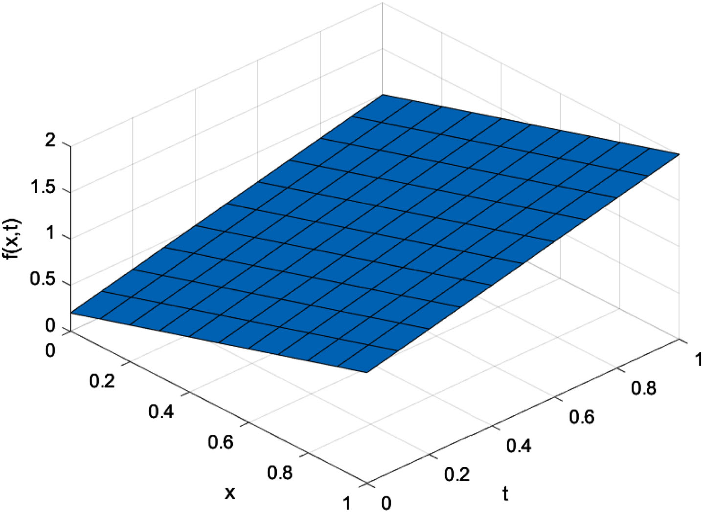
$\begin{matrix} f (x, t) = f_{0} (x, t) + f_{1} (x, t) + f_{2} (x, t) + f_{3} (x, t) + . . . \\ f (x, t) = x + 1 - α + t α . \end{matrix}$

Notice that as α → 1, we have f (x, t) = x + t which is the exact solution of the ordinary initial value problem.

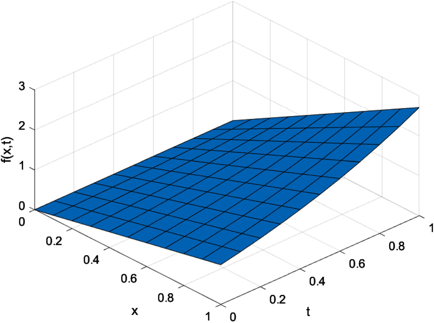
Figures 2 illustrate the graphs of analytic solutions at α = 1 and α = 0.8 for Example 1, respectively. It is clear from Figures 2 that the solution of Example 1 increases linearly as x and t increase.

Fig. 1

Truncated solution of Example 1 for α = 1.

Fig. 2

Truncated solution of Example 1 for α = 0.8.

Example 2. Let us consider the following linear TFIVP: $_{0}^{C F} D_{t}^{α} f (x, t) = - \frac{\partial}{\partial x} (x f (x, t)) + \frac{\partial^{2}}{\partial x^{2}} (\frac{x^{2} f (x, t)}{2}),$ (8) $f (x, 0) = x .$ (9) Utilization of the ARA transform for (8) produces the following: $\begin{matrix} G_{1} [f (x, t)] (s) = f (x, 0) + (1 - α + \frac{α}{s}) G_{1} \\ [- \frac{\partial}{\partial x} (xf (x, t)) + \frac{\partial^{2}}{\partial x^{2}} (\frac{x^{2} f (x, t)}{2})] (s) . \end{matrix}$ At this stage, applying the inverse ARA transform leads to the following:

$\begin{matrix} f (x, t) = G_{1}^{- 1} [f (x, 0)] + G_{1}^{- 1} [(1 - α + \frac{α}{s}) G_{1} \\ [- \frac{\partial}{\partial x} (xf (x, t)) + \frac{\partial^{2}}{\partial x^{2}} (\frac{x^{2} f (x, t)}{2})] (s)] \end{matrix}$ which implies the following recurrence relations:

$\begin{matrix} f_{0} (x, t) = G_{1}^{- 1} [f (x, 0)] = x, \\ f_{1} (x, t) = G_{1}^{- 1} [(1 - α + \frac{α}{s}) G_{1} [- \frac{\partial}{\partial x} ({xf}_{0} (x, t)) \\ + \frac{\partial^{2}}{\partial x^{2}} (\frac{x^{2} f_{0} (x, t)}{2})] (s)], \\ f_{1} (x, t) = x (1 - α + α t), \\ f_{2} (x, t) = G_{1}^{- 1} [(1 - α + \frac{α}{s}) G_{1} [- \frac{\partial}{\partial x} (x (f_{0} + f_{1})) \\ + \frac{\partial^{2}}{\partial x^{2}} (\frac{x^{2} (f_{0} + f_{1})}{2})] (s)] \\ - G_{1}^{- 1} [(1 - α + \frac{α}{s}) G_{1} [- \frac{\partial}{\partial x} ({xf}_{0}) \\ + \frac{\partial^{2}}{\partial x^{2}} (\frac{x^{2} f_{0}}{2})] (s)], \\ f_{2} (x, t) = x ((1 - 2 α + α^{2}) + \frac{t^{2} α^{2}}{2} + t (2 α - 2 α^{2})), \end{matrix}$

$\begin{matrix} f_{3} (x, t) = G_{1}^{- 1} [(1 - α + \frac{α}{s}) G_{1} \\ [- \frac{\partial}{\partial x} (x (f_{0} + f_{1} + f_{2})) \\ + \frac{\partial^{2}}{\partial x^{2}} (\frac{x^{2} (f_{0} + f_{1} + f_{2})}{2})] (s)] \\ - G_{1}^{- 1} [(1 - α + \frac{α}{s}) G_{1} [- \frac{\partial}{\partial x} (x (f_{0} + f_{1})) \\ + \frac{\partial^{2}}{\partial x^{2}} (\frac{x^{2} (f_{0} + f_{1})}{2})] (s)], \\ f_{3} (x, t) = x (1 - 3 α + 3 α^{2} - α^{3} + \frac{t^{3} α^{3}}{6} \\ + t^{2} (\frac{α}{2} + α^{2} - \frac{3 α^{3}}{2}) + t (1 + α - 5 α^{2} + 3 α^{3})), \\ f_{4} (x, t) = G_{1}^{- 1} [(1 - α + \frac{α}{s}) G_{1} \\ [- \frac{\partial}{\partial x} (x (f_{0} + f_{1} + f_{2} + f_{3})) \\ + \frac{\partial^{2}}{\partial x^{2}} (\frac{x^{2} (f_{0} + f_{1} + f_{2} + f_{3})}{2})] (s)] \\ - G_{1}^{- 1} [(1 - α + \frac{α}{s}) G_{1} [- \frac{\partial}{\partial x} (x (f_{0} + f_{1} + f_{2})) \\ + \frac{\partial^{2}}{\partial x^{2}} (\frac{x^{2} (f_{0} + f_{1} + f_{2})}{2})] (s)], \end{matrix}$

$\begin{matrix} f_{4} (x, t) = x (1 - 4 α + 6 α^{2} - 4 α^{3} + α^{4} + \frac{t^{4} α^{4}}{24} \\ + t (3 α - 10 α^{2} + 11 α^{3} - 4 α^{4}) \\ + t^{3} (- \frac{α^{3}}{6} + \frac{1}{6} (α^{2} + 4 α^{3} - 4 α^{4})) \\ + t^{2} (- \frac{α}{2} - \frac{3 α^{2}}{2} + \frac{3 α^{3}}{2} \\ + \frac{1}{2} (2 α + 6 α^{2} - 13 α^{3} + 6 α^{4}))) . \end{matrix}$ As a result, a truncated solution of the TFIVP (8)-(9) is established as follows: $\begin{matrix} f (x, t) = f_{0} (x, t) + f_{1} (x, t) + f_{2} (x, t) + f_{3} (x, t) + . . . \end{matrix}$

$\begin{matrix} f (x, t) = x + x (1 - α + α t) \\ + x ((1 - 2 α + α^{2}) + \frac{t^{2} α^{2}}{2} + t (2 α - 2 α^{2})) \\ + x (1 - 3 α + 3 α^{2} - α^{3} + \frac{t^{3} α^{3}}{6} \\ + t^{2} (\frac{α}{2} + α^{2} - \frac{3 α^{3}}{2}) + t (1 + α - 5 α^{2} + 3 α^{3})) \\ + x (1 - 4 α + 6 α^{2} - 4 α^{3} + α^{4} + \frac{t^{4} α^{4}}{24} \\ + t (3 α - 10 α^{2} + 11 α^{3} - 4 α^{4}) \\ + t^{3} (- \frac{α^{3}}{6} + \frac{1}{6} (α^{2} + 4 α^{3} - 4 α^{4})) \\ + t^{2} (- \frac{α}{2} - \frac{3 α^{2}}{2} + \frac{3 α^{3}}{2} \\ + \frac{1}{2} (2 α + 6 α^{2} - 13 α^{3} + 6 α^{4}))) + . . . \end{matrix}$

Notice that as α → 1, we have $\begin{matrix} f (x, t) = x (1 + t + \frac{t^{2}}{2} + \frac{t^{3}}{6} + \frac{t^{4}}{24} + . . .) = {xe}^{t} \end{matrix}$ which is the exact solution of the ordinary initial value problem.

Figures 4 illustrate the graphs of analytic and truncated solutions at α = 1 and α = 0.8 for Example 2, respectively. As it can be seen from Figures 4, the solution increases linearly as x increases and increases nonlinearly as t increases.

Fig. 3

Truncated solution of Example 2 for α = 1.

Fig. 4

Truncated solution of Example 2 for α = 0.8.

Now we compare truncated solution of example 2 with truncated solution, obtained by Laplace homotopy analysis method (LHAM) in Table 1.

It is obvius from Table 1 that the results of proposed method is much more better than the results of LHAM [24] which illustrates the accuracy and effectiveness of the proposed method.

Table 1

The results of proposed method and LHAM at x = 0.05, and their comparison at α = 1 for Example 2

	α = 1	α = 1	α = 1	α = 1	α = 1
t	Proposed method	LHAM	Exact solution	Proposed method	LHAM
				\|v_app - v_exact\|	\|v_LHAM - v_exact\|
0.01	0.050502508354167	0.0500025	0.050502508354208	4.172356904419416 × 10^-14	4.9502 × 10^-3
0.05	0.052563554687500	0.0500625	0.052563554818801	1.313011990800028 × 10^-10	2.5011 × 10^-3
0.1	0.055258541666667	0.0502502	0.055258545903782	4.237115713845441 × 10^-9	5.0083 × 10^-3
0.15	0.058091679687500	0.0505636	0.058091712136414	3.244891415288276 × 10^-8	7.5281 × 10^-3
0.2	0.061070000000000	0.0510033	0.061070137908009	1.379080084920603 × 10^-7	1.0066 × 10^-3

Example 3. Let us consider the following non-linear TFIVP: $_{0}^{C F} D_{t}^{α} f (x, t) = - \frac{\partial}{\partial x} ((\frac{4 f (x, t)}{x} - \frac{x}{3})) + \frac{\partial^{2}}{\partial x^{2}} (f^{2} (x, t)),$ (10) $f (x, 0) = x^{2} .$ (11) where α ∈ (0, 1] , x, t ∈ (0, 1). Utilization of the ARA transform for (10) produces the following: $\begin{matrix} G_{1} [f (x, t)] (s) = f (x, 0) + (1 - α + \frac{α}{s}) G_{1} [ \\ - \frac{\partial}{\partial x} ((\frac{4 f (x, t)}{x} - \frac{x}{3}) f (x, t)) \\ + \frac{\partial^{2}}{\partial x^{2}} (f^{2} (x, t))] (s) . \end{matrix}$ At this stage, applying the inverse ARA transform leads to the following: $\begin{matrix} f (x, t) = G_{1}^{- 1} [f (x, 0)] + G_{1}^{- 1} [(1 - α + \frac{α}{s}) \\ G_{1} [- \frac{\partial}{\partial x} ((\frac{4 f (x, t)}{x} - \frac{x}{3}) f (x, t)) \\ + \frac{\partial^{2}}{\partial x^{2}} (f^{2} (x, t))] (s)] \end{matrix}$ which indicates the following recurrence relations:

$\begin{matrix} f_{0} (x, t) = G_{1}^{- 1} [f (x, 0)] = x^{2}, \\ f_{1} (x, t) = G_{1}^{- 1} [(1 - α + \frac{α}{s}) G_{1} \\ [- \frac{\partial}{\partial x} ((\frac{4 f_{0}}{x} - \frac{x}{3}) f_{0}) + \frac{\partial^{2}}{\partial x^{2}} (f_{0}^{2})] (s)], \\ f_{1} (x, t) = x^{2} (1 - α + α t), \\ f_{2} (x, t) = G_{1}^{- 1} [(1 - α + \frac{α}{s}) G_{1} [ \\ - \frac{\partial}{\partial x} ((\frac{4 (f_{0} + f_{1})}{x} - \frac{x}{3}) (f_{0} + f_{1})) \\ + \frac{\partial^{2}}{\partial x^{2}} ({(f_{0} + f_{1})}^{2})] (s)] \\ - G_{1}^{- 1} [(1 - α + \frac{α}{s}) G_{1} \\ [- \frac{\partial}{\partial x} ((\frac{4 f_{0}}{x} - \frac{x}{3}) f_{0}) + \frac{\partial^{2}}{\partial x^{2}} (f_{0}^{2})] (s)], \\ f_{2} (x, t) = x^{2} (1 - 2 α + α^{2} + t (2 α - 2 α^{2}) + \frac{t^{2} α^{2}}{2!}), \end{matrix}$ $\begin{matrix} f_{3} (x, t) = G_{1}^{- 1} [(1 - α + \frac{α}{s}) G_{1} [ \\ - \frac{\partial}{\partial x} ((\frac{4 (f_{0} + f_{1} + f_{2})}{x} - \frac{x}{3}) (f_{0} + f_{1} + f_{2})) \\ + \frac{\partial^{2}}{\partial x^{2}} ({(f_{0} + f_{1} + f_{2})}^{2})] (s)] \\ - G_{1}^{- 1} [(1 - α + \frac{α}{s}) G_{1} [ \\ - \frac{\partial}{\partial x} ((\frac{4 (f_{0} + f_{1})}{x} - \frac{x}{3}) (f_{0} + f_{1})) \\ + \frac{\partial^{2}}{\partial x^{2}} ({(f_{0} + f_{1})}^{2})] (s)], \\ f_{3} (x, t) = x^{2} (1 - 3 α + 3 α^{2} - α^{3} \\ + (3 α - 6 α^{2} + 3 α^{3}) t + (2 α^{2} - 2 α^{3}) t^{2} + \frac{α^{3} t^{3}}{3}) . \end{matrix}$

As a result, a truncated solution of the TFIVP (10)-(11) is established as follows:

$\begin{matrix} f (x, t) = f_{0} (x, t) + f_{1} (x, t) + f_{2} (x, t) + . . . \\ f (x, t) = x^{2} + x^{2} (1 - α + α t) \\ + x^{2} (1 - 2 α + α^{2} + t (2 α - 2 α^{2}) + \frac{t^{2} α^{2}}{2!}) \\ + x^{2} (1 - 3 α + 3 α^{2} - α^{3} \\ + (3 α - 6 α^{2} + 3 α^{3}) t + (2 α^{2} - 2 α^{3}) t^{2} + \frac{α^{3} t^{3}}{3}) + . . . \end{matrix}$

Notice that as α → 1, we have $\begin{matrix} α \to 1, f (x, t) = x^{2} (1 + t + \frac{t^{2}}{2!} + \dots) = x^{2} e^{t} . \end{matrix}$ which is the exact solution of the ordinary initial value problem.

Figures 6 illustrate the graphs of analytic and truncated solutions at α = 1 and α = 0.8 for Example 3, respectively. It is obvious from Figures 6 that the solution of Example 3 increases nonlinearly as x and t increase.

Fig. 5

Truncated solution of Example 3 for α = 1

Fig. 6

Truncated solution of Example 3 for α = 0.8

5 Conclusion

A new method is proposed and analyzed by combining the ARA transform and iterative method. The existence of the ARA transform is investigated. Moreover, it is shown that the ARA integral transform of order n of a continuous function is well-defined. This proposed method is utilized to establish truncated or analytic solutions of linear or non-linear TFIVP with the Caputo-Fabrizio derivative. In this method, we first apply the ARA transform and its inverse transform to reduce the problem, and then the iterative method is applied to construct a truncated solution. ARA transform is an effective transformation for fractional differential equations, significantly contributing to the proposed method. Moreover, it can be concluded from illustrative examples with the Fokker-Planck equation that this method is applicable and effective compared to the other methods. In future research, the ARA transform will be combined with another numerical method to develop new methods for fractional differential equations with various fractional derivatives.

References

Kodal Sevindir

, Cetinkaya

and Demir

, On effects of a new method for fractional initial value problems, Advances in Mathematical Physics 2021 (2021), ArticleID7606442.

Cetinkaya

and Demir

, On the solution of Bratu’s initial value problem in the Liouville-Caputo sense by ARA transform and decomposition method, Comptes rendus de l’Academie bulgare des Sciences 74(12) (2021), 1729–1738.

El-Sayed

A.M.A.

, Elsaid

, El-Kalla

I.L.

, et al., A homotopy perturbation technique for solving partial differential equations of fractional order in finite domains, Appl Math Comput 218 (2012), 8329–8340.

Elsaid

, Homotopy analysis method for solving a class of fractional partial differential equations, Commun Nonlinear Sci 16 (2011), 3655–3664.

Turut

and Güzel

, On solving partial differential equations of fractional order by using the variational iteration method and multivariate pad'e approximations, Eur J Pure Appl Math 6 (2013), 147–171.

Cetinkaya

, Demir

and Kodal

, Sevindir, Solution of space-time-fractional problem by shehu variational iteration method, Advances in Mathematical Physics 2021 (2021), ArticleID5528928.

Khalouta

and Kadem

, Comparison of new iterative method andnatural homotopy perturbation method for solving nonlineartime-fractional wave-like equations with variable coefficients, Nonlinear Dyn Syst Theory 19 (2019), 160–169.

Podlubny

, Fractional Differential Equations, Academic Press, New York, 1999.

Saadeh

, Qazza

and Burqan

, A new integral transform: ARA transform and its properties and applications, Symmetry 12 (2020).

10.

Caputo

and Fabrizio

, A new definition of fractional derivative without singular kernel, Progress in Fractional Differentiation and Applications 1(2) (2015), 73–85.

11.

Ahmad

, Ullah

and Akgul

, Study of a fractional system of predator-prey with uncertain initial conditions, Mathematical Problems in Engineering 2022 (2022), ArticleID3196608.

12.

Gulalai , Ahmad

, Rihan

F.A.

, Ullah

, Al-Mdallal

Q.M.

and Akgul

, Nonlinear analysis of a nonlinear modified KdV equation under Atangana Baleanu Caputo derivative, AIMS Mathematics 7(5) (2022), 7847–7865.

13.

Ahmad

, Ullah

, Akgul

and Jarad

, A hybrid analytical technique for solving nonlinear fractional order PDEs of power law kernel: Application to KdV and Fornberg-Witham equations, AIMS Mathematics 7(5) (2022), 9389–9404.

14.

Alqahtani

R.T.

, Ahmad

and Akgul

, Dynamical analysis of bio-ethanol production model under generalized nonlocal operator in caputo sense, Mathematics 9(19) (2021), 1–21.

15.

Losada

and Nieto

J.J.

, Fractional integral associated to fractional derivatives with nonsingular kernels, Progr Fract Differ Appl 7(3) (2021), 137–143.

16.

Caputo

and Fabrizio

, On the singular kernels for fractional derivatives, some applications to partial differential equations, Progr Fract Differ Appl 7(2) (2021), 79–82.

17.

Fabrizio

and Pecoraro

, The yield effect in viscoplastic materials, A Mathematical Model, Zeitschrift Für Angewandte Mathematik und Physik 70(1) (2019), Articlenumber:25.

18.

Atanacković

T.M.

, Pilipović

and Zorica

, Properties of the Caputo-Fabrizio fractional derivative and its distributional settings, Fractional Calculus and Applied Analysis 21 (2018), 29–44.

19.

Enelund

and Olsson

, Damping described by fading memory–analysis and application to fractional derivative models, International Journal of Solids and Structures 36(7) (1999), 939–970.

20.

Singh , Kumar

, Purohit

S.D.

, Mishra

A.M.

and Bohra

, An efficient numerical approach for fractional multidimensional diffusion equations with exponential memory, Numerical Methods for Partial Differential Equations 37(2) (2021), 1631–1651.

21.

Phuong

N.D.

, Hoan

L.V.C.

, Karapinar

, Singh

, Binh

H.D.

and Can

N.H.

, Fractional order continuity of a time semilinear fractional diffusion-wave system, Alexandria Engineering Journal 59(6) (2020), 4959–4968.

22.

Singh , Kumar

and Baleanu

, A new analysis of fractional fish farm model associated with Mittag-Leffler-type kernel, International Journal of Biomathematics 13(2) (2020), Article2050010.

23.

Losada

and Nieto

J.J.

, Properties of a new fractional derivative without singular kernel, Progr Fract Differ Appl 1(2) (2015), 87–92.

24.

Korpinar

, Inc

and Baleanu

, On the fractional model of Fokker-Planck equations with two different operator, AIMS Mathematics 5(1) (2019), 236–248.

25.

Risken

, The Fokker–Planck Equation: Method of Solution and Applications, Springer, Berlin, 1989.