Handling similar looking disease symptoms in plants using dilation and feature reuse

Abstract

For the last decade, the use of deep learning techniques in plant leaf disease recognition has seen a lot of success. Pretrained models and the networks trained from scratch have obtained near-ideal accuracy on various public and self-collected datasets. However, symptoms of many diseases found on various plants look similar, which still poses an open challenge. This work takes on the task of dealing with classes with similar symptoms by proposing a trained-from-scratch shallow and thin convolutional neural network employing dilated convolutions and feature reuse. The proposed architecture is only four layers deep with a maximum width of 48 features. The utility of the proposed work is twofold: (1) it is helpful for the automatic detection of plant leaf diseases and (2) it can be used as a virtual assistant for a field pathologist to distinguish among classes with similar symptoms. Since dealing with classes with similar-looking symptoms is not well studied, there is no benchmark database for this purpose. We prepared a dataset of 11 similar-looking classes and 5, 108 images for experimentation and have also made it publicly available. The results demonstrate that our proposed model outperforms other recent and state-of-the-art models in terms of the number of parameters, training & inference time, and classification accuracy.

Keywords

Plant disease similar-looking symptoms shallow CNN models lightweight models agriculture

1 Introduction

Agriculture is considered an important portion of a country’s economy. To increase crop yield and ensure quality production, crop health monitoring and necessary remedial actions are inevitable. With recent developments in the field of precision agriculture [1], modern farming techniques and effective use of sensors [2] have improved agricultural production [3]. Adoption of new technology trends has become common among farmers around the globe to handle various issues inhibiting the growth of crops from both biotic and abiotic classes. The best defense a farmer has against such plant diseases is proper diagnosis, timely treatment, and control measures [4].

Right now, the most common diagnostic technique is to visually analyze the evident symptoms that may occur due to the presence of abiotic and biotic factors like pests or fungi but automatic diagnosis using computer vision techniques is also in practice for the last decade or so. Scientists have used various approaches based on conventional machine learning and deep learning to address this issue with the latter being more common. Famous deep learning approaches include but are not limited to compression [5] and implementation of efficient networks [6]. The first approach [7] uses quantization and pruning methods in the pre-trained networks and hence compresses the model several times. The others implement efficient structures to design lightweight networks that provide competitive accuracy on resource-constrained devices for plant disease recognition [8]. MobileNet [9], SqueezeNet [10] and Inception [11] or residual blocks are used for this purpose. In recent years, smartphones have immensely increased in almost every field. Moreover, with the success of computer vision techniques in the field of disease diagnosis especially in agriculture. State-of-the-art contributions have been made to improve the implementation of such effective methods for plant disease classification and detection [12]. Many researchers used feature, color, and texture information from parts of a plant suffering from various diseases [13]. Better detection performances were obtained by using already trained and modified CNN (Convolutional Neural Networks) models [14]. Remarkable progress has been made to classify and detect disease symptoms from real-world scenes. This led to the use of GPUs (Graphical Processing Units) or TPUs (Tensor Processing Units) to train deep models like VGG16 [15], ResNets [16], and DenseNet [17]. These models outperformed all other existing feature-engineered methods but are accompanied by the issues like large memory and computational cost issues.

Apart from the computational cost imposed by the deep learning models, plant disease recognition suffers from other challenges like similarity in the visual characteristics of images. In many practical situations, different diseases are presented with similar-looking symptoms which can confuse even an expert pathologist [18]. Figure 1 shows three cases where different diseases produce similar-looking symptoms for tomato, mango, and wheat plants. Mosaic virus (at an early stage) and nutrition deficiency look similar to each other on tomato leaves as shown in Fig. 1(a). Similarly, on mango plant, salt injury and anthracnose are presented with symptoms that look alike at varying disease stages (Fig. 1(b)). Moreover, Fig. 1(c) shows images of the leaves infected by three diseases namely stem rust, brown rust and yellow rust on wheat plant. It can be seen that the symptoms of the three are visually very close to each other.

Fig. 1

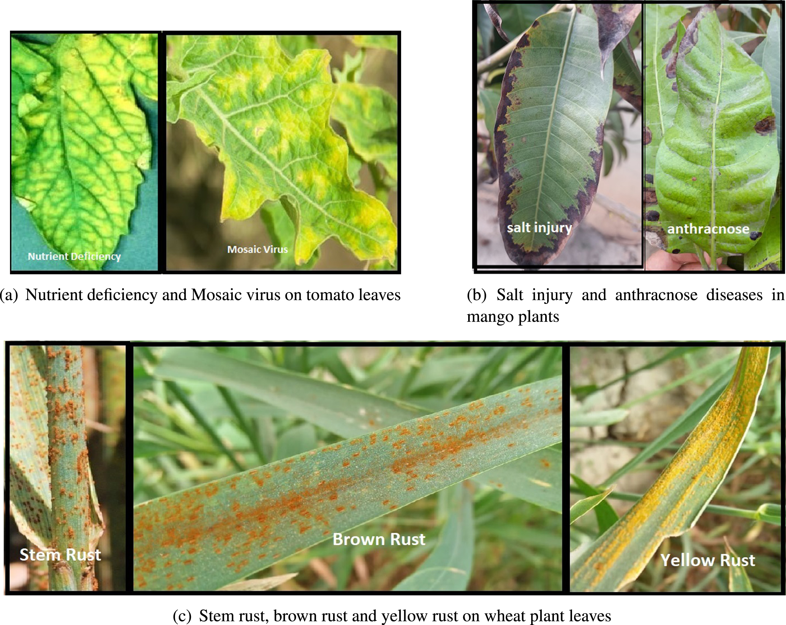
Visually similar-looking symptoms of disease (best seen in color).

A careful analysis of the recent and state of the art literature suggests that the problem of handling the case where different classes are presented with similar-looking symptoms is a least addressed topic. We, in this work, present a computationally efficient deep learning model to address the issue of similar-looking disease symptoms. We employ atrous convolutions and additive feature reuse to preserve intricate feature details. To achieve better performance and efficiency on limited computational resources the model is kept thin and shallow. The performance of the proposed model is evaluated to classify similar-looking plant diseased symptoms using a self-collected dataset. Major contributions of this research are as follows:

To propose a shallow thin model that could efficiently perform plant disease diagnosis. For this purpose, feature reuse and dilated convolution were explored to collect intricate features explicitly.

To collect and present a unique dataset that addresses a common yet least addressed problem i.e., similar-looking foliar symptoms of various plants.

The rest of this paper is organized in the following sequence. Section 2 summarizes the recent literature work related to our problem. The proposed methodology is discussed in Section 3. Experimentation and results are given in Section 5. Finally, Section 6 concludes the work and discusses future work.

2 Related work

There are two types of computer vision models applied by researcher to recognize plant leaf diseases namely machine learning and deep learning. The former are conventional methods but today have fairly been replaced by deep learning methods because of better accuracy and performance on specialized hardware.

Convolutional neural networks (CNNs), a special type of deep learning models especially designed for image processing, effectively extract robust features from input images instead of relying on manually selecting features. Transfer learning-based approaches (that utilize a pretrained CNN) have been extensively used by researchers [19–21]. Deeper networks like ResNets, VGG-16, DenseNets, and Inception models have been implemented to segment and visualize features related to plant stress and disease [14]. The fine-tuned or trained from scratch models have remarkable accuracies which come at computational cost [22]. Recent trends in plant disease recognition have drastically shifted towards achieving better computational efficiency. In a noticeable work by Hu et al. [23], a method was proposed to identify tea leaf diseases with low cost and high accuracy. Depthwise separable convolutions were used in addition to multiscale feature extraction methods to achieve better convergence CNN as compared to VGG16 and AlexNet. A pruned version of MobileNet was presented by Kamal et al. in [24]. The significance of the depthwise separable convolution in achieving better convergence and accuracy with reduced parameters was expressed using the PlantVillage dataset. Reasonable accuracy results along with low memory requirements were fulfilled by an efficient 8-layer deep CNN model proposed by Agarwal et. al [25]. The proposed light-weight model was obtained by compressing the VGG16 model. The attention-based deep residual network was designed to detect tomato diseases with an accuracy of 98% using effective feature extraction technique [26]. In another work, model compression based on tensor decomposition was performed to evaluate real-time grape leaf diseases. Model superiority was calculated based on memory occupancy and inference time.

CNN based models can either be learnt from scratch or can be transfer learned. All the above-mentioned works have focused on feature extraction using transfer learned deeper networks which require immense fine-tuning and computations. A recent trend is to train shallow and light networks from scratch. Yang et al. [27] combined a shallow CNN for feature extraction and machine learning classifiers to recognize plant leaf diseases. The model outperformed other deep CNN models based on several metrics. Also, a novel energy-efficient thin network is trained and validated for traffic sign recognition by Haque et al. [28]. Many authors have used transfer learned light-weight models for analysis on specific datasets [21, 29]. Inference time, trainable parameters, model size, and time to converge were considered as key evaluation metrics in designing low-power low-cost CNN models. To reduce the number of FLOPs and model size, several techniques have been adopted like weight quantization [30], pruning [31], low-rank decomposition, and knowledge-distillation. The latter technique has been effectively implemented by Wenjie et al. [32] to perform the recognition task of 38 crop diseases. The knowledge from trained teacher model VGG16 was transferred to the student MobileNet model; reducing the inference time of the distilled model for the same accuracy performance. A novel plant disease detection CNN was presented by Wang et al. [33] by compressing VGG and AlexNet. The scheme improvised pruning to remove redundant parameters, knowledge distillation to get accuracy, and weight compression to reduce model size. A lightweight CNN was developed for wheat disease classification using inverted residual block with attention mechanism [34]. The model with only 2.1M parameters identified diseased regions from real-field images with an accuracy of 94.1%. An efficiently scaled dilated convolution neural network was proposed by Poudel et al. [35] to classify similar looking colorectal disease images. The authors further used a DropBlock regularization with a transfer-learned Resnet-50 baseline architecture. The similarity of diseased symptoms is as common in biomedical imaging as it is in plants. Dilated convolutions were used to classify skin diseases having less inter-class variance [36]. The authors combined the advantages of the hybrid loss function and leaky ReLu to diagnose skin lesions with 94.7% accuracy.

Keeping in view the different approaches used by the researchers to achieve hardware compatibility and real-time latency for specific agricultural applications, we, in this work, propose a shallow model trained from scratch for our specific application. The proposed model utilizes additive feature reuse extracted by dilated convolutions from bottom layer. Global average pooling and smaller feature maps are effectively incorporated to combat overfitting [37]. The simpler thin model is validated and compared on the basis of various metrics. A dataset comprising of 11 classes of similar-looking diseases of mango, wheat, grapes, and potatoes was also collected and used for experiments.

3 The proposed methodology

A low-cost shallow model is trained from scratch for our application-specific task to efficiently identify visually similar-looking disease symptoms in plants. Instead of making the CNN deeper or wider, intricate spatial features are extracted using dilated convolutions and efficiently incorporating them by using skip connections and feature reuse in adjacent layers. The prime motivation is to address the problem of similar-looking symptoms by minimizing the number of parameters and computations. It is generally achieved either by reducing the feature map size or by limiting the number of convolution and hidden layers. By doing so, we tend to avoid overfitting that generally occurs because of over-parametrization in sequential layers. With the requirement to extract essential features with fewer computations, we have used a smaller kernel size fixed at 3 × 3 in all convolutional layers. The proposed architecture has only four stages of convolutional layers with a width of 48 feature maps. The model hence is shallow, thin [28] computationally efficient and accurate at the same time. The CNN architecture is trained from scratch and validated on our similar-looking plant disease dataset. The overall flow of the proposed approach in identifying diseased symptoms in plants is shown in Fig. 2.

Fig. 2

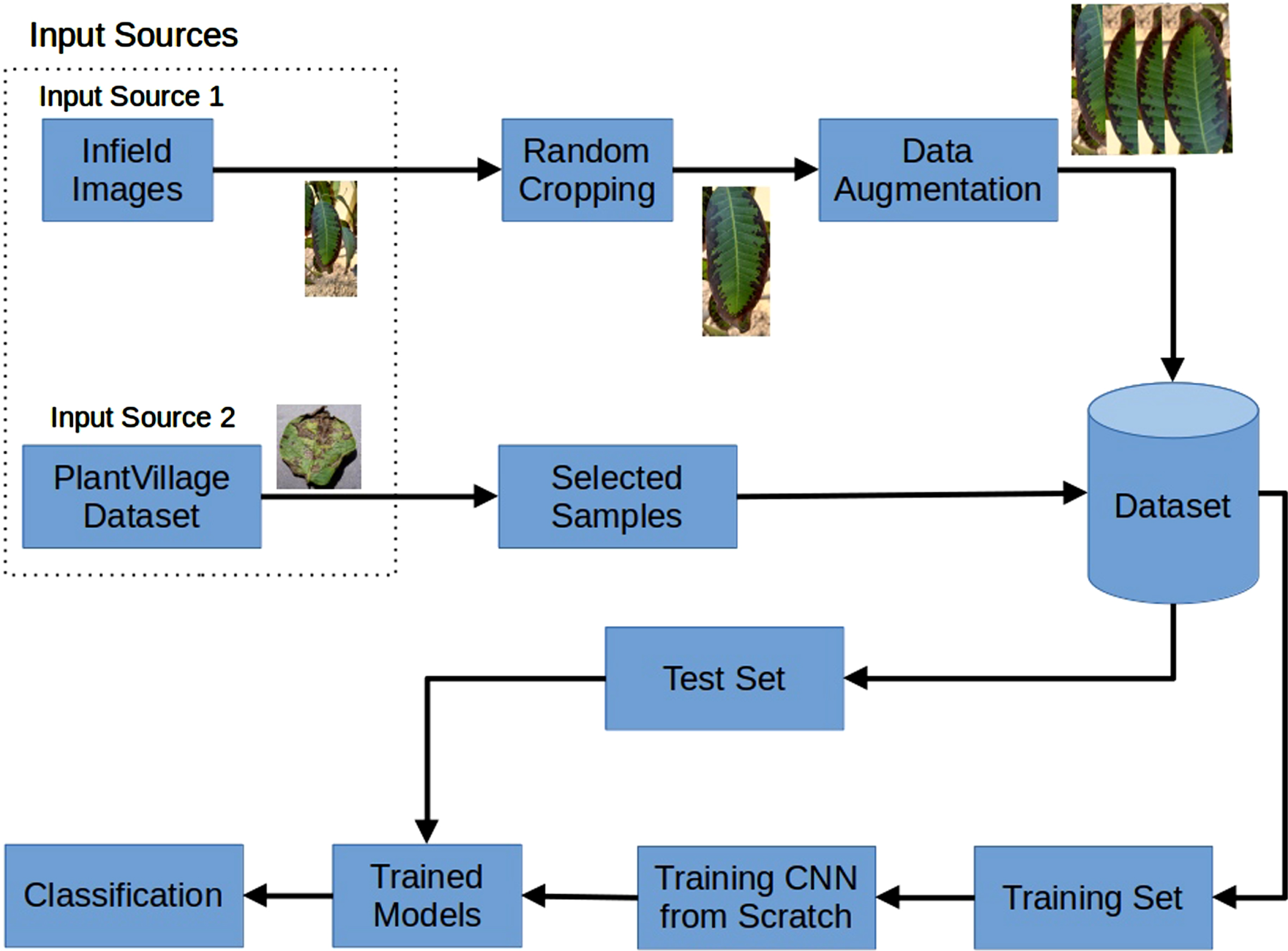
Overall flow diagram of the proposed CNN model.

Fig. 3

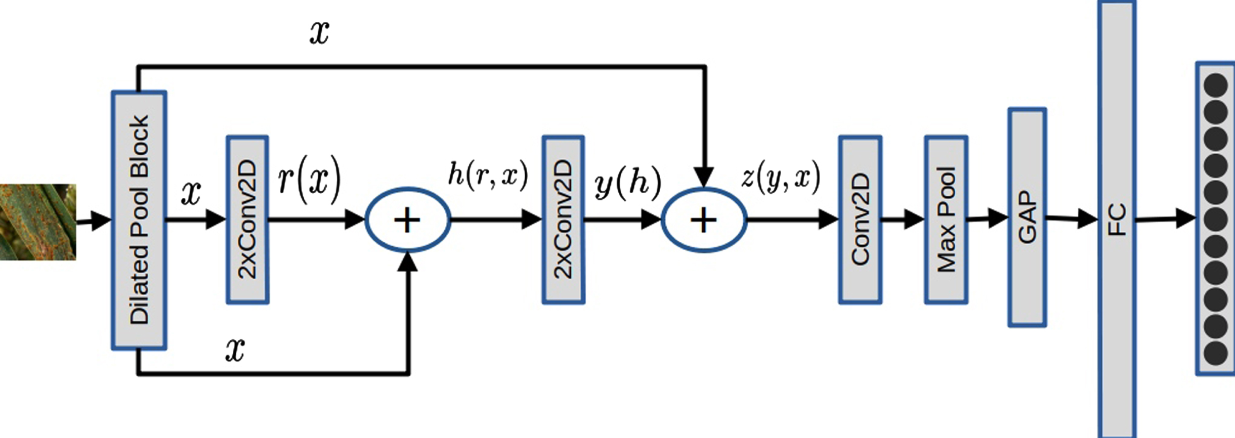
Block diagram of the proposed model, internal details of the Dilated Pool Block are given in Fig. 4.

3.1 Dilated convolution

In order to preserve spatial information of low-level features we have efficiently used dilation [38] with effectively reusing them in later layers [35]. In our four-layered model, the intricate features differentiating similar-looking classes are preserved and later systematically down-sampled. The receptive field of the input image, I, is increased by employing an expanded kernel f. The dilated kernel has holes between its consecutive elements. Convolutional operation is performed in the same way as traditional convolutional operation along with a parameter l showing the number of elements skipped in the kernel as shown in Equation (1). $(I_{* l} f) (p) = \sum_{(s + lt = p)} I (s) f (t)$ (1)

where input image I (s) is convolved with kernel f (t). l is dilation rate which l=1 for simple convolution giving output image I_*f (p) and I_*2f (p) for l=2. The receptive field of I₂ is produced from I₁ which is 1-dilated. The receptive field for dilated convolution can be calculated by Equation (2). $I_{(i + 1)} = (2^{i + 2} - 1) \times (2^{i + 2} - 1)$ (2)

The receptive field of dilated convolution block shown in Fig. 4 is given by Equation (3). We have used dilated convolution in first two convolutional layers with an atrous rate of 2. $I_{2} = (2^{1 + 2} - 1) \times (2^{1 + 2} - 1)$ (3)

As I₂ is derived from Equation (2) where, i = 1 for 2-dilated convolution, hence, the receptive field of each element in I₂ becomes 7 × 7. The method offers a wider field of view with approximately the same computational cost. The size of the receptive field increases exponentially as mentioned in Equation (2) and hence the cost increases linearly [38].

Fig. 4

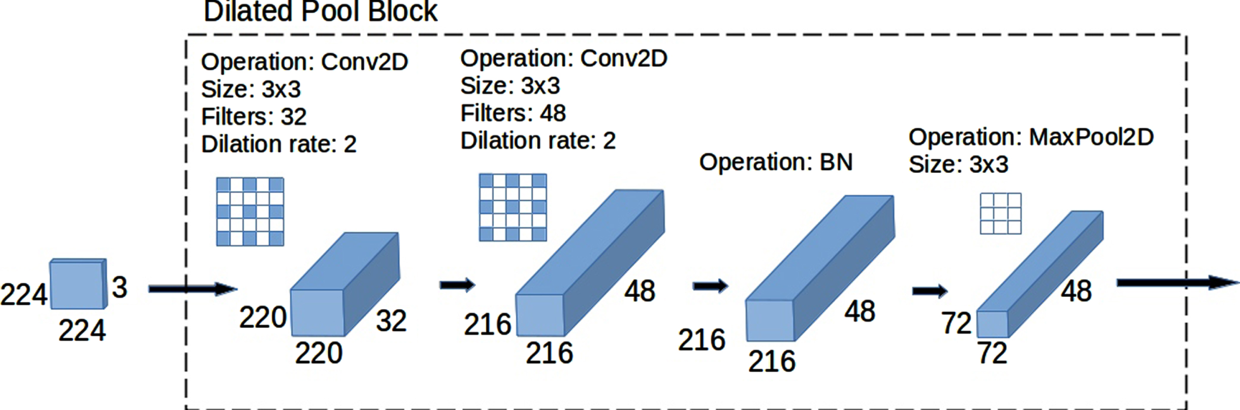
Illustration of the Dilated Pool Block employed in our proposed technique demonstrated in Fig. 3.

Our proposed dilated pool block as shown in Fig. 4 is comprised of two layers of convolution at a dilation rate of 2 along with the ReLu activation function. Valid padding is used in these convolutions as our images are captured in real conditions and padding will add noise to the extracted feature maps. The shape and size of convolutions will remain the same after applying the dilation. The first layer generates a feature map of 220 × 220 × 32 and after applying 48 filters in the next convolution it becomes 216 × 216 × 48. The feature map after applying the activation function is normalized by applying batch normalization as given in Equation (4). $N_{l}^{f} = \frac{I_{l}^{f} - μ_{B}}{\sqrt{σ^{2} + ϵ}}$ (4)

where $N_{l}^{f}$ is the normalized feature map, $I_{l}^{f}$ is the input feature map μ_B, and σ² are the mean and variance of mini-batch respectively used to perform standardization. ϵ is added as a very small number to avoid any zero in the denominator. Max pool operation highlights the most distinguishing feature in the respective patch. As for our case, we need to downsample our feature map for the next stage keeping the most discriminant information so we apply a 3 × 3 filter to generate a map of 72 × 72 × 48.

3.2 Feature reuse

The proposed model contains a dilated-pool block and three convolutional layers, a global average pooling layer, and one fully connected layer as shown in Fig. 3. The input to the model is in the form of a tensor which is represented as in Equation (5) $(image, I) = (η_{h}, η_{w}, η_{c})$ (5)

where h, w, and c are the height, width, and channel parameters of the image. C = 3 for an RGB image. A square kernel F with the same number of channels C is slided over the input image resulting in a 2-dimensional tensor G (x, y) as shown in Equation (6) $\begin{matrix} G (x, y) & = Conv (I, F)_{(x, y)} \\ = \sum_{i = 1}^{η_{h}} \sum_{j = 1}^{η_{w}} \sum_{k = 1}^{η_{c}} F_{i, j, k} I_{x + i - 1, y + j - 1, k} \end{matrix}$ (6)

The dimensions of output, G (x, y), is defined as: $[G (x, y)]_{(\frac{η_{h} + 2 p - f}{s} + 1) \times (\frac{η_{w} + 2 p - f}{s} + 1)}$ (7)

where p = padding, which is p = 0 for valid padding, s stands for stride that is generally 1 and f is kernel size that is 3. Convolution operation calculates a dot product of kernel receptive field values and its respective weights followed by ReLu activation which is one of the most commonly used function that returns the same value as input and zero for all values less than zero, i.e., g (x) = max (0, x). Learning process starts from input to output layer in forward propagation by setting weights and bias values. The process involves updating weights by applying any gradient decent algorithm by minimizing cost function J. $J (θ) = \frac{1}{n} \sum_{i = 1}^{n} (L y_{i}^{θ}, y_{i})$ (8)

n is the size of training set with ${\hat{y}}_{i}^{θ}$ is the predicted class computed for x_i and θ are the model parameters updated in every epoch i. The loss function L is the distance between real and predicted class values, which is calculated using cross-entropy loss expressed in Equation (9). $L (y_{i}^{θ}, y_{i}) = (y_{i} \log (y_{i}^{θ}) + (1 - y_{i}) \log (1 - y_{i}^{θ}))$ (9)

Gradient descent algorithms are applied to update the parameters with value, ω_i. $ω_{i}^{s} quo = ω_{i} + Δ ω_{i}$ (10) $Δ ω_{i} = - λ \frac{\partial L}{\partial Δ ω_{i}}$ (11)

λ is the learning rate and L is the loss function. The parameters of each layer are updated with the rule mentioned in Equation (11). During back-propagation, the loss function is iteratively optimized by adjusting the layer parameters. By performing these partial derivatives for several iterations, hence loss function is reduced enough. A vanishing gradient occurs when the gradient reaches a value where it further stops improving the weights. The phenomena commonly occur in deeper networks which researchers previously overcome by several methods like fine-tuning or stopping further training of the network. Skip connections provide a win-win situation for CNN to escape this decreasing gradient problem. ResNet was the first to use it [16]. The technique allows to preserve the gradient of few layers and later on reuse it either by addition or concatenation. Feature information can be preserved by performing concatenation operative in adjacent layers [17]. The residual block resulting from skip connections is given by H (x), which is the output of the block. R (x) is the output resulting from convolution operation performed in the preceding layer i, i.e., τr (x, W_i). where W_i is the weight matrix of the previous layers. $h (r, x) = r (x) + x$ (12)

where Equation (12) shows addition operation of any input x with transform function τ after non-linear operation in preceding layers. The resultant output vector learned will be y (h) input to the next transformation layer; which is again a convolution operation followed by ReLu activation. $z (y, x) = y (h) + x$ (13)

The skip and concatenated connections allow feature reusability effectively. Feature information extracted generally in starting layers is lost sometimes during down-sampling and may suffer from vanishing gradient problem. Hence such residual connection allows using the most important feature information at some later stage. The spatial information extracted by using atrous convolution in the dilated-pool block is later reused at layers 2 and 3 as shown in Fig. 3. Computational cost is preserved by restricting the feature maps. Further details of the architecture proposed in Section 3.3.

3.3 Low-cost shallow model

In this study, we designed a low-cost shallow network for our specific application i.e., to recognize and distinguish between images processing visually identical symptoms at varying disease stages. Layer-wise detailed architecture of our proposed system is depicted in Fig. 3. The network is only 4 layers deep and is designed with a small number of feature maps; hence making it thin at the same time. Less number of parameters and reduced complexity made the model be used on resource constraint devices. The specialized dilated pool block explained in Section 3.1 is used for the specific task of identifying discriminating features for the particular dataset. Following the dilated pool block, the pooled feature map is passed through two convolutional layers each followed by activation. We have zero-padded these two convolutional layers to avoid losing any spatial details from the boundaries. The output of these convolutional blocks is added with the feature map of dilated pool block using skip connection as shown in Fig. 3 and shown by Equation (12). In order to keep the model robust against gridding effects and noise, downsampling is necessary. Max-pooling operation is performed with a window of 2 × 2. Global Average pooling is used to convert the multidimensional feature map to 1D tensor. The individual elements in the feature map no longer contain any spatial arrangement of input features. Moreover, before the fully connected classification layers, we need to flatten our feature maps. Global average pooling performs the task of flattening by selecting a global mean value from the feature map. Hence the most distinguishable features are averaged out before softmax classification as shown in Fig. 5.

Fig. 5

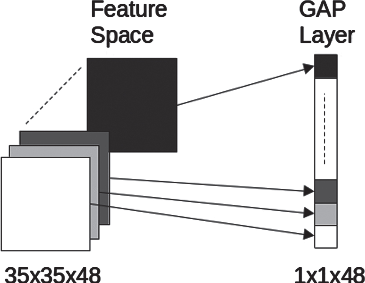
Global Average pooling as flatten layer.

To avoid the network from getting overfit, we have adopted a few traditional techniques. Apart from data augmentation, we have adopted dropout with the fully connected layers. By applying the dropout regularization, we chose L_N × P_N × k in the forward path inside the hidden layers (where L_N is the number of input layer neurons, P_N the output layer neurons and k is a parameter whose value varies from 0 to 1). To save the best model, we have used checkpoint callbacks after every epoch to save the best weights for maximum validation accuracy.

Cross-entropy loss was used as a performance measure and is calculated as: $loss = - \sum_{n = 1}^{N} \sum_{c = 1}^{C} t_{i_{c}} \log (y_{i}) c$ (14) where C denotes total number of classes and N shows total number of samples. Further, y_i is the probability that i^th sample belongs to an arbitrary class c and t_{i
_c} is a Boolean variable whose value is equal to 1 if it belongs to class c and 0 otherwise. The cross-entropy loss function is calculated for every iteration and weights are updated accordingly.

Algorithm 1. Algorithm to extract features for similarlooking symptoms.

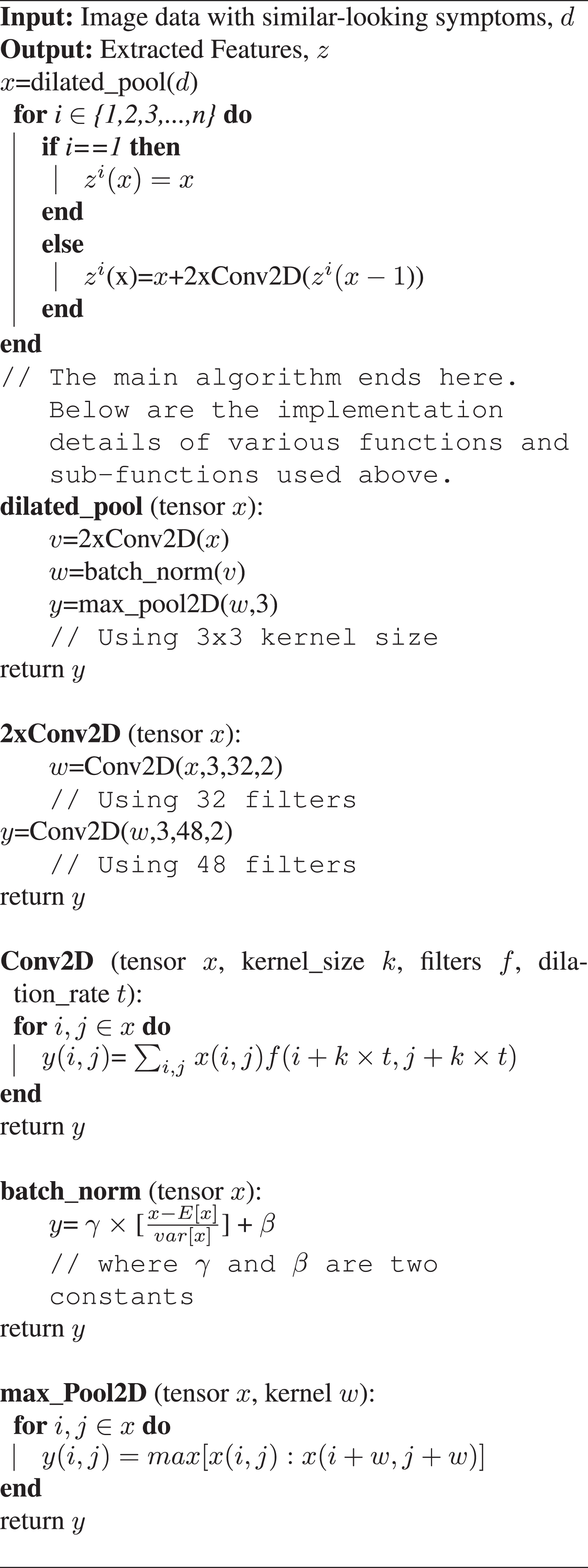
Finally, the proposed feature extraction technique, capable of generating discriminating features in the presence of similar-looking symptoms, is described as a pseudocode in Algorithm 1. Coarsely, it is a two step process i.e., dilated pooling followed by additive 2 × Conv2D recursively. The dilated pooling operation involves 2 × Conv2D, batch normalization and then a a max pooling operation. The operation 2 × Conv2D takes an image tensor as input and two conventional Conv2D operations are performed in series with 32 and 42 filters respectively. Kernel size is kept at 3 whereas the dilation rate is fixed at 2. Recursive additive-convolution mentioned in Algorithm 1 is an operation where the output of the dilated pool block is added to the 2 × Conv2D operation performed on current image tensor. The algorithm shows that the operation should be performed for values of n from 1 to any arbitrarily chose value n. However, for the sake of this study, we used n = 3 and found it empirically optimal. Increasing n beyond this value adds to the computational complexity of the algorithm and doesn’t provide any benefit as far as the overall performance is concerned.

4 Dataset

4.1 Image acquisition

The images obtained in our work are collected from Multan, Bahawalpur and Rawan cities of southern Punjab region, Pakistan. The image acquisition process was started from March 2021 to September 2021. The collection span was chosen based on wheat, mango growth characteristics and disease occurrence and its progress on the particular host. To replicate a real-time disease recognition system the image acquisition was only performed by hand held smartphones (Samsung A31s and A20) in varying lighting conditions i.e., the images were captured from 1.00pm to 4pm. Out of the 496 images in total, 452 were shortlisted after discarding blurred and poorly illuminated ones. Apart from these we have taken some images from PlantVillage dataset.

4.2 Image preprocessing and augmentation

Our proposed dataset captured wheat and mango leaf images in real-field conditions. Random cropping is performed by using bounding box information on the self collected dataset. In this data augmentation technique, random subset of image is collected. By using LabelImg tool for bounding box information, single leaf image was cropped from a real-field image containing complex information of background. The advantage of doing so will help our CNN learn object of interest, as our particular case focuses to distinguish between disease symptoms which require to use a cropped dataset that can be compared with PlantVillage images. By using this cropping technique we have created an augmented subset of original real-world dataset. It is because we want our deep learning model to learn details of disease symptoms not the cluttered background details. The cropped images are further enhanced by using data augmentation techniques. The image is cropped keeping the lesion region in focus as shown in Fig. 6.

Fig. 6

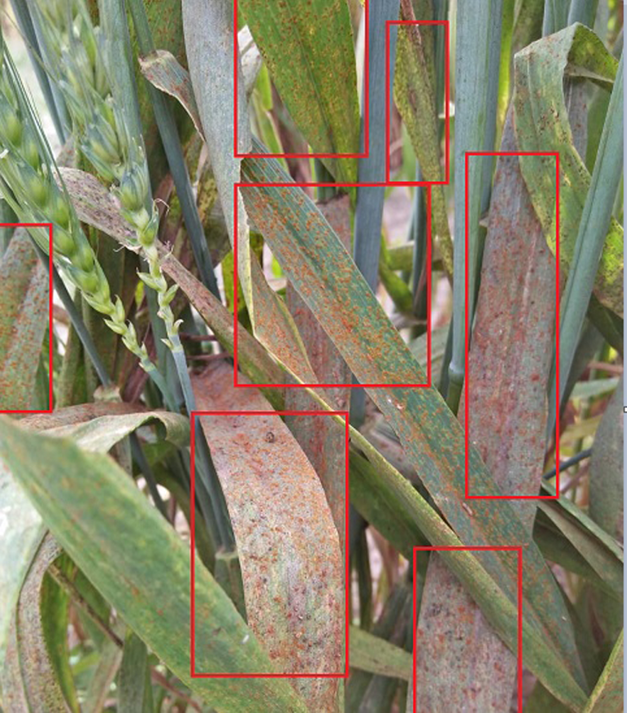
Cropped images from real-field captured scenario.

After applying cropping, contrast adjustment was performed. Images captured under natural & field conditions often suffer light/color intensity variations. We have collected 5 classes of wheat out of which 3 possess similar-looking features and 2 classes of mango explained in Tables 2. The number of collected images from field was limited because of human effort and limitations involved in collecting and annotating data samples. Hence, the training models were generalized by increasing the data. Offline transformations like horizontal & vertical flip and rotation [-15°, 0, 15°] were performed to diversify the training samples. To further diversify the dataset, 4 similar-looking classes of PlantVillage were also added. Table 1 describes those disease classes that look visually similar alongwith type of agent causing it. As the plantVillage images contain single leaf image so preprocessing is not applied on them. The sample images of our collected dataset is shown in Fig. 7. The 5, 108 cropped & augmented images were further divided into 70% training, 20% validation and 10% test data. The details of which are shown in Table 2.

Fig. 7

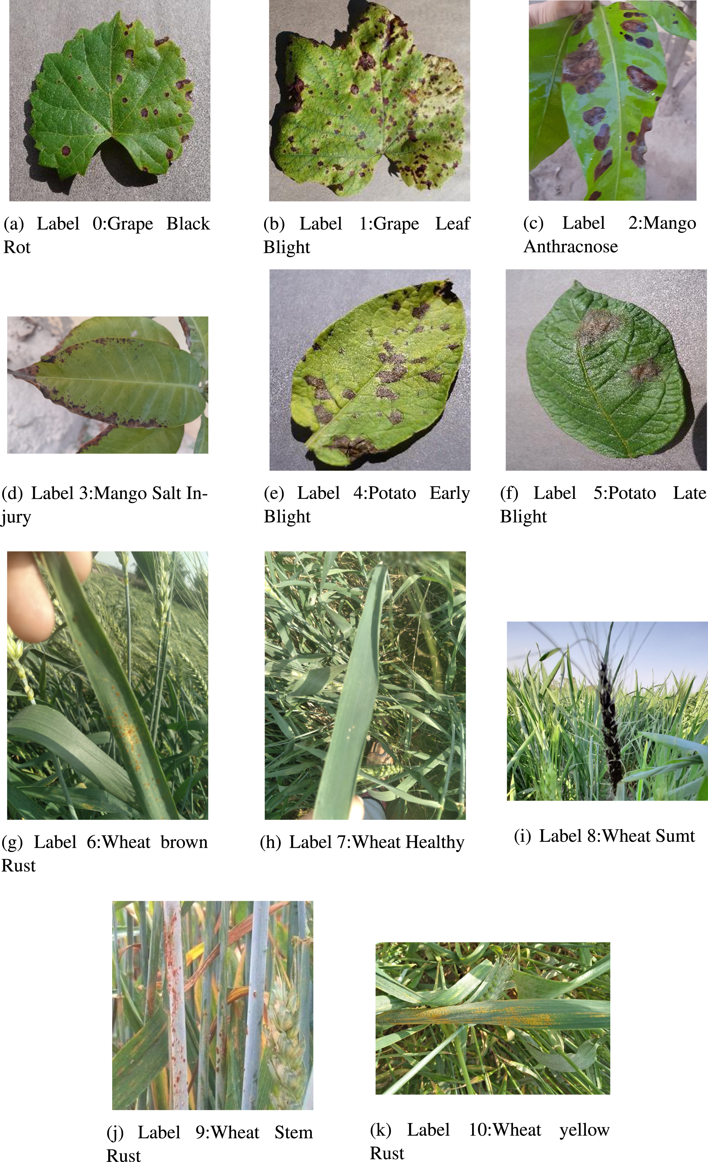
Sample images of Similar looking plant disease symptoms dataset.

Table 1

Details of the similar-looking symptoms of few plants covered in our dataset

Disease	Agent	Symptoms	Typical Host(s)	Affected Area
Brown rust	Puccinia triticina	Dusty reddish-orange to reddish-brown spots	Wheat, Maize, Barley	Leaf
Yellow rust	Puccinia striiformis	Yellow-orange pustles arranged in the form of stripes	Wheat, Maize, Barley	Leaf, Awns, Glumes
Stem Rust	Puccinia graminis	Orange-red elongated oval shaped lesions	Wheat, Maize, Barley	Stem, Leaf, Glumes, Awns
Anthracnose	Glomerella cingulata	Irregular blister like brown spots on tips, margins of leaves	Mango, Walnut, Maple	Twigs, Fruits
Salt injury	Water, Potassium deficiency, Salt excess	Tip burning in necrotic regions and edges	Mango, Corn, Tomato	Leaves, Stem
Black Rot	Guignardia bidwellii	Brown circular and elongated black lesions	Grape	Leaves, Fruits
Leaf Blight	Pseudocercospora vitis	Dull red lesions turns black	Grapes	Leaves, Fruit
Early Blight	Alternaria solani	Dark irregular lesions with yellow borders	Potato, Tomato	Leaves, Tubers
Late Blight	Phytophthora infestans	Dark blotches that later turn gray and reddish brown	Potato, Tomato	Leaves, Tubers

Table 2

Details of the dataset used in the proposed work

Label No.	Class	Training Images	Validation images	Test images
0	Grape Black Rot	347	99	50
1	Grape Leaf Blight	347	99	51
2	Mango Anthracnose	351	34	17
3	Mango Salt Injury	352	34	17
4	Potato Early Blight	322	92	46
5	Potato Late Blight	291	83	42
6	Wheat Brown Rust	427	40	21
7	Wheat Healthy	440	42	21
8	Wheat Smut	414	40	20
9	Wheat Stem Rust	354	34	17
10	Wheat Yellow Rust	426	41	20
	Total	4093	693	322

5 Experimental details

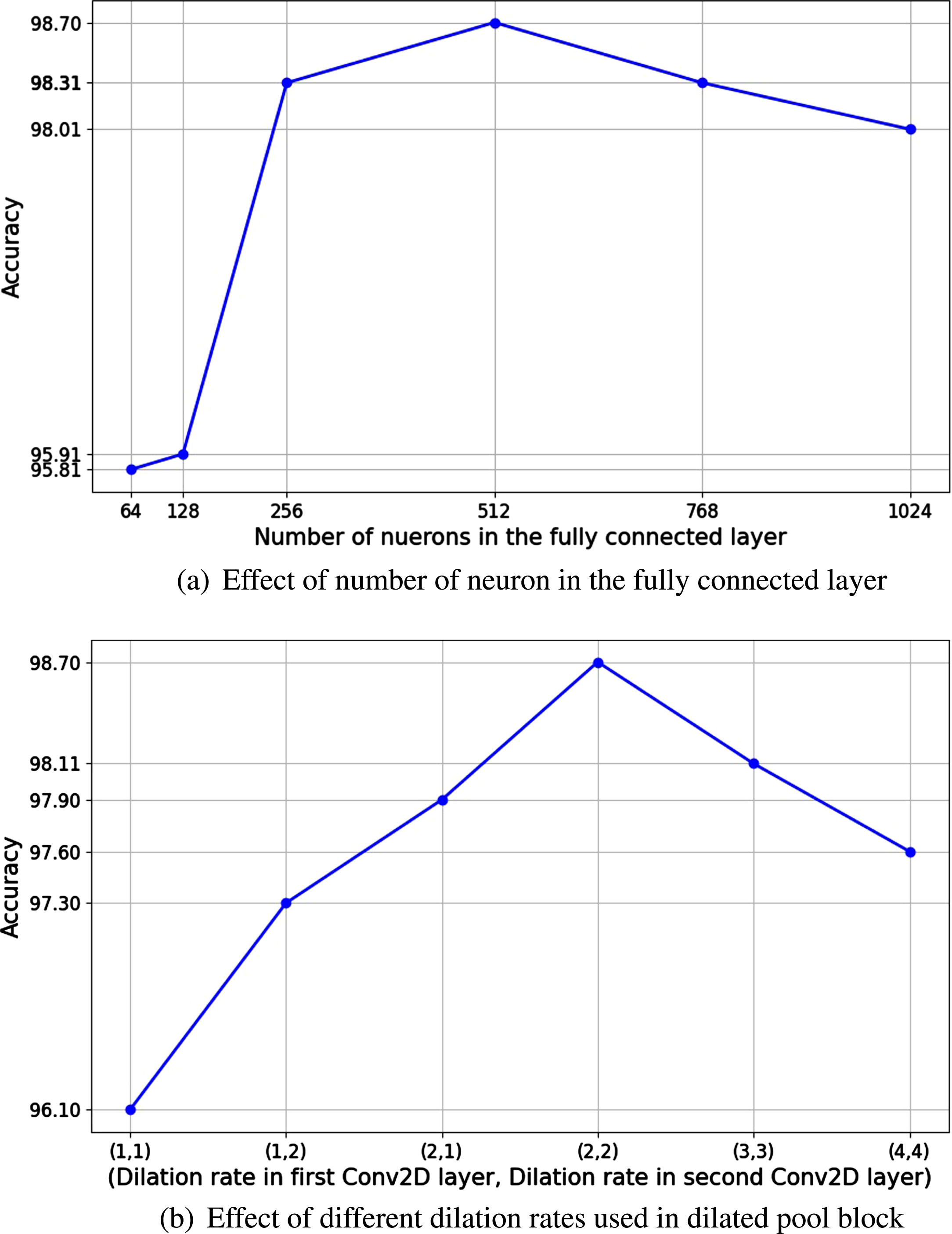
To validate the performance of the proposed CNN on our application, we used a self-collected dataset from the field discussed in Section 4. We performed several empirical calculations and conducted several experiments to reach an optimal architecture in terms of computations and classification accuracy. The essence of CNN architectures is that they need several tweaks in terms of hyper-parameters and the placement of several layers to get the best results. To make a shallow and thin network in pursuance to reach best results at a minimum cost we have performed the experiments with the following experimental settings:

The resolution of images and sizes may vary because of variation in shooting devices. The size of images at the input size is set to 224 × 224 × 3.

Filter size is set to 3 × 3 in all convolutional layers was empirically found to be the best option. We have stacked two convolutional layers to get the smallest features with a small kernel size. Instead of using a large kernel size on one convolutional layer. The technique not only helps us to achieve optimal classification performance but also balances the trainable parameters. However, the receptive field is increased by using dilation. Best results were obtained for dilation rate=2 in the dilated pool block. The effect of varying dilation rates on recognition accuracy is shown in Fig. 8(b).

Fig. 8

Analysis of proposed CNN architecture for varying parameters.

Number of filters in convolutional layers are optimally selected. The number of filters is limited to 48 in an attempt to make the architecture low cost and thin.

The proposed model uses only one fully connected layer to avoid overfitting in optimal training time. The number of neurons in the fully connected layer is fixed to 512. Global average pooling layer is used instead of Batch Normalization and fully connected layers. It is will make the network less prone to overfitting and lead to early convergence [39].

The proposed CNN model is trained on back-propagation learning using Adam optimizer. The learning rate is decreased using the annealing technique with starting value set to 1 × 10^-3. The overall summary of proposed deep learning model is shown in Table 3.

We have also compared our proposed model with other state-of-the-art models on the basis of depth, width, trainable parameters, and other evaluation metrics mentioned in Section 5.2 The training of proposed model for was performed in 895seconds.

After the model fine-tuning, we performed the model training and validation on the similar-looking symptoms dataset. The results obtained using 322 test images are compared with other deep transfer learned models based on accuracy.

Table 3

Summary of the proposed deep learning model

Layer Type	Kernel	Channels	Output size	Parameters
Input			224 × 224 × 3	0
Conv2D	3 × 3	32	220 × 220 × 32	896
Conv2D_1	3 × 3	48	216 × 216 × 48	13,872
Batch Normalization			216 × 216 × 48	192
MaxPool	3 × 3		72 × 72 × 48	0
2×Conv2D_2	3 × 3	48	72 × 72 × 48	41, 568
Add			72 × 72 × 48	0
Conv2D_3	3 × 3	48	72 × 72 × 48	20, 784
Add_1			72 × 72 × 48	0
Conv2D_4	3 × 3	48	70 × 70 × 48	20, 784
MaxPool	2 × 2		35 × 35 × 48	0
Global Avg Pool			1 × 1 ×48	0
Fully Connected			1 × 1 ×512	25,088
Dropout(50%)			1 × 1 ×512	0
Fully Connected (Classification)			1 × 1 ×11	5643
Total parameters: 128, 827
Trainable parameters: 128, 731
Non-trainable parameters: 96

The proposed framework is implemented, trained, and validated on Keras using 12 GB GPU on Intel Core i3 1.20GHz using 8.GB RAM.

5.1 Ablation study

To analyze the effect of network components and understand the result on model performance, an ablation study is performed whose results are given in Table 4. Accuracy and F1 values are examined by systematically considering experimental variables. These variables are kept as 512 number of neurons in the fully connected layer, dropout of 50%, dilation rate of 2, and feature reuse is performed on adjacent layers as shown in Fig. 3. In Table 4, "√" means the module is added and "×" means not added in the model. The best performance in terms of accuracy and F1 score can be seen in strategy 4 complying with the efficacy of our proposed technique to classify similar-looking classes. Moreover, Figs. 8(a) & 8(b) further elaborate the effect of varying number of neurons and dilation rates on model performance respectively.

Table 4
Results of the ablation study conducted on our proposed technique

Strategy 512 Neurons in FC Layer Feature Reuse Dropout 0.50 Dilation (2,2) Accuracy F1-score

1 √ × × × 95.12 0.94

2 √ √ × × 97.55 0.96

3 √ √ √ × 98.10 0.98

4 √ √ √ √ 98.70 0.99

Strategy	512 Neurons in FC Layer	Feature Reuse	Dropout 0.50	Dilation (2,2)	Accuracy	F1-score
1	√	×	×	×	95.12	0.94
2	√	√	×	×	97.55	0.96
3	√	√	√	×	98.10	0.98
4	√	√	√	√	98.70	0.99

5.2 Results and analysis

So far we have evaluated the model classification accuracy and its performance in evaluating classes having less inter-class variance. The proposed shallow & thin architecture is critically tuned and its parameters are adjusted considering varying filter size, dilation rates, and the number of neurons in fully connected layers. Experimentation concluded that Adam optimizer effectively calculates the optimal value for the model.

So now we can further proceed to extend our comparison to other existing deep learning approaches. For a fair comparison, we have considered deep networks like ResNet50 and VGG19; lightweight networks like MobileNet and MobileNetV2, and state-of-the-art DenseNet121 model which are deep as well as uses the concatenation approach in their architecture. The comparison of classification accuracy, trainable parameters, time, and depth of the model are also summarized in Table 5. For the case of VGG19, the network fails to converge and could not work well considering its baseline model. ResNet50 achieves 98.11 accuracy at the cost of trainable parameters. MobileNet V2 performed the best while achieving an overall accuracy comparable to our proposed model with the minimum number of parameters as can be seen in Fig. 9. Clearly, our proposed CNN achieves comparable classification results with minimum number of trainable parameters as other deep learningmodels.

Fig. 9

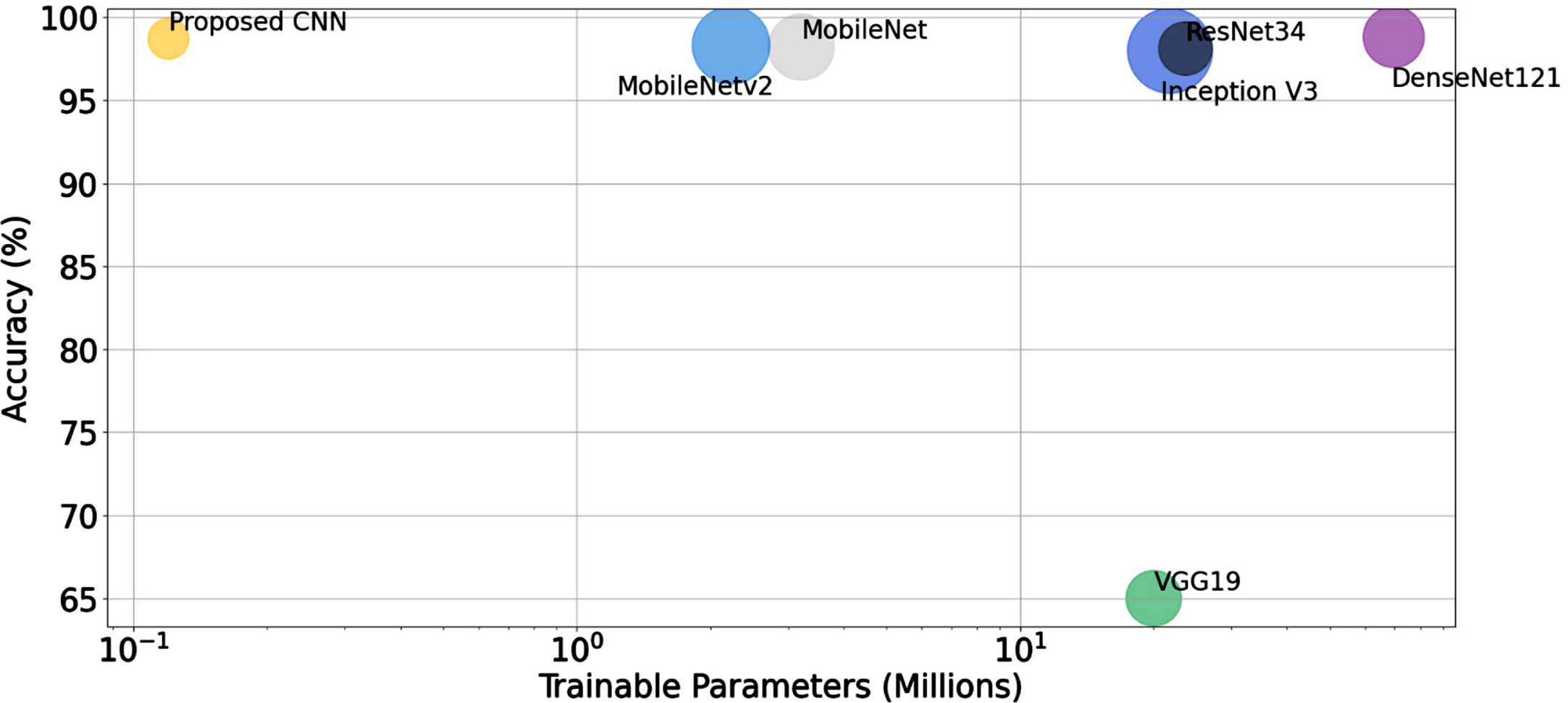
Comparison of trainable parameters and training accuracy of proposed CNN with other deep learning models.

The proposed model is trained for 60 epochs keeping in view the size and classes of the dataset, the batch size of 16 is used. Considering our specific application, the CNN model was expected to distinguish between similar-looking classes. For this purpose, various metrics were used to measure the performance of the model, and comparison was established with other deep learning transfer learned models. All the models chosen are trained on the imageNet weights with the top layer removed. Average pooling is performed and optimum weight selection is performed using Adam optimizer. Figure 10(a) shows confusion matrix of our proposed CNN model. Before identifying the False-positive and negatives, we must recall that class 0 & class 1 are similar-looking classes as shown by the yellow rectangular box in Fig. 10(a). Moreover, class 2 & class 3, class 4 & class 5 and class 6, class 9 & class 10 are the classes having less inter-class variance. A set of similar-looking classes are highlighted with the rectangular box to analyze mis-classifications amongst them. Our proposed model correctly classified between grape black rot & leaf blight and for potato early blight and late blight too; no false correlations are seen. Mango anthracnose is mis-classified only once with mango salt injury. Classes 6, 7, and 8 are similar-looking classes of wheat brown, stem, and yellow rust. Our model distinguishes among them having 2 false positives of class 6 with class 9 and class 10. Although the accuracy performance of MobileNetV2 is the same with a comparable number of parameters in the confusion matrix shown in Fig. 10(b), we see that more mis-classifications are observed between similar classes. It shows that our model has the capability to correctly discriminate and classify similar-lookingclasses.

Fig. 10

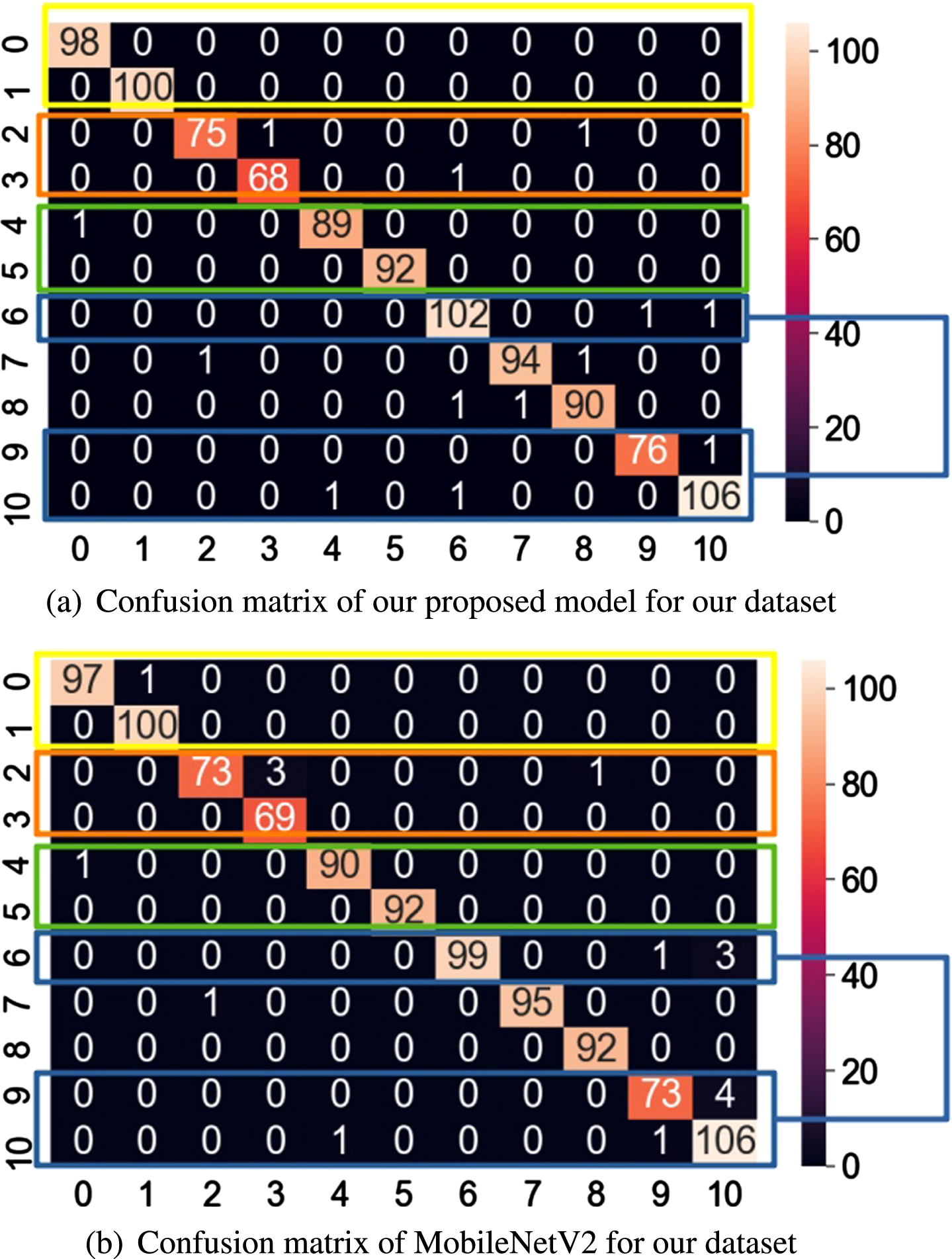
Classification performance analysis for similar looking classes.

Table 5

Comparison of the identification results of the proposed model with other deep learning models.

Model	Accuracy (%)	Trainable Parameters (M)	time/epoch (Sec)	depth
VGG19	65	20.03	46	26
ResNet34	98.11	23.61	28	20
DenseNet121	98.81	69.65	30	121
MobileNet	98.20	3.21	24	88
MobileNetV2	98.31	2.23	23	88
Inception V3	97.98	21.8	24	159
Proposed CNN	98.70	0.12	14	4

6 Conclusion and future work

In this work, a shallow thin CNN architecture was proposed for the classification of visually similar-looking plant disease symptoms that are often difficult to identify even by expert pathologists. Although the model is shallow but effective use of dilation in bottom layers and feature reuse in a sequenced manner made the model distinguish between classes having less inter-class variance. Since the field is least addressed in the literature, there is no public dataset comprising of disease classes with similar-looking inter class symptoms. We, as part of this work, have developed a rich dataset specific to this problem.

We intend to extend this work by effectively incorporating depth-wise separable convolutions to make the model more computationally lightweight. Moreover, the network parameters and architectures will be explored further to reduce the mis-classification between the classes. Further, we also intend to enhance our self collected dataset reported in this paper by adding images from various disease severity stages.

Footnotes

Appendix

References

Kamilaris

and Prenafeta-Boldú

F.X.

, Deep learning in agriculture: A survey, Computers and Electronics in Agriculture 147 (2018), 70–90.

and Yang

G.-H.

, Data-based distributed sensor scheduling for multiple linear systems with H performance preservation, IEEE Transactions on Automatic Control (2021).

Saleem

M.H.

, Potgieter

and Arif

K.M.

, Automation in agriculture by machine and deep learning techniques: A review of recent developments, Precision Agriculture (2021), 1–39.

Barbedo

J.G.A.

, Digital image processing techniques for detecting, quantifying and classifying plant diseases, Springer-Plus 2(1) (2013), 1–12.

Qin

, Liu

, Huang

, Wu

and Zhang

, LeanNet: An efficient convolutional neural network for digital number recognition in industrial products, Sensors 21(11) (2021), 3620.

, Zhang

, Li

, Lv

and Tong

, Efficient densely connected convolutional neural networks, Pattern Recognition 109 (2021), 107610.

Han

, Mao

and Dally

W.J.

, Deep compression: Compressing deep neural networks with pruning, trained quantization and huffman coding, arXiv preprint arXiv:1510.00149 (2015).

Thakur

P.S.

, Sheorey

and Ojha

, VGG-ICNN: A Lightweight CNN model for crop disease identification, Multimedia Tools and Applications 82(1) (2023), 497–520.

Howard

A.G.

, Zhu

, Chen

, Kalenichenko

, Wang

, Weyand

, Andreetto

and Adam

, Mobilenets: Efficient convolutional neural networks for mobile vision applications, arXiv preprint arXiv:1704.04861 (2017).

10.

Iandola

F.N.

, Han

, Moskewicz

M.W.

, Ashraf

, Dally

W.J.

and Keutzer

, SqueezeNet: AlexNet-level accuracy with 50x fewer parameters and <0.5 MB model size, arXiv preprint arXiv:1602.07360 (2016).

11.

Szegedy

, Ioffe

, Vanhoucke

and Alemi

A.A.

, Inception-v4, inception-resnet and the impact of residual connections on learning, in: Thirty-First AAAI Conference on Artificial Intelligence 2017.

12.

Noon

S.K.

, Amjad

, Qureshi

M.A.

and Mannan

, Use of deep learning techniques for identification of plant leaf stresses: A review, Sustainable Computing: Informatics and Systems 28 (2020), 100443.

13.

Pydipati

, Burks

and Lee

, Statistical and neural network classifiers for citrus disease detection using machine vision, Transactions of the ASAE 48(5) (2005), 2007–2014.

14.

Saleem

M.H.

, Potgieter

and Arif

K.M.

, Plant disease detection and classification by deep learning, Plants 8(11) (2019), 468.

15.

Yang

, Ni

, Gao

, Han

and Luan

, A novel method for peanut variety identification and classification by Improved VGG16, Scientific Reports 11(1) (2021), 1–17.

16.

, Zhang

, Ren

and Sun

, Deep residual learning for image recognition, in: Proceedings of the IEEE Conference on Computer Vision and Pattern Recognition 2016, pp. 770–778.

17.

Huang

, Liu

, Van Der Maaten

and Weinberger

K.Q.

, Densely connected convolutional networks, in: Proceedings of the IEEE Conference on Computer Vision and Pattern Recognition (2017), 4700–4708.

18.

Noon

S.K.

, Amjad

, Qureshi

M.A.

and Mannan

, Handling severity levels of multiple co-occurring cotton plant diseases using improved YOLOX model, IEEE Access 10 (2022), 134811–134825.

19.

Chen

, Chen

, Zhang

, Sun

and Nanehkaran

Y.A.

, Using deep transfer learning for image-based plant disease identification, Computers and Electronics in Agriculture 173 (2020), 105393.

20.

Mohanty

S.P.

, Hughes

D.P.

and Salathé

, Using deep learning for image-based plant disease detection, Frontiers in Plant Science 7 (2016), 1419.

21.

Noon

S.K.

, Amjad

, Qureshi

Ali M.

and Mannan

, Computationally light deep learning framework to recognize cotton leaf diseases, Journal of Intelligent & Fuzzy Systems (2021), 1–16.

22.

Liu

and Wang

, Plant diseases and pests detection based on deep learning: A review, Plant Methods 17(1) (2021), 1–18.

23.

, Yang

, Zhang

and Wan

, Identification of tea leaf diseases by using an improved deep convolutional neural network, Sustainable Computing: Informatics and Systems 24 (2019), 100353.

24.

Kamal

, Yin

, Wu

and Wu

, Depthwise separable convolution architectures for plant disease classification, Computers and Electronics in Agriculture 165 (2019), 104948.

25.

Agarwal

, Gupta

S.K.

and Biswas

, Development of efficient CNN model for Tomato crop disease identification, Sustainable Computing: Informatics and Systems 28 (2020), 100407.

26.

Karthik

, Hariharan

, Anand

, Mathikshara

, Johnson

and Menaka

, Attention embedded residual CNN for disease detection in tomato leaves, Applied Soft Computing 86 (2020), 105933.

27.

, Nie

and Chao

, Do we really need deep CNN for plant diseases identification? Computers and Electronics in Agriculture 178 (2020), 105803.

28.

Haque

W.A.

, Arefin

, Shihavuddin

and Hasan

M.A.

, DeepTh: A novel lightweight CNN architecture for traffic sign recognition without GU requirements, Expert Systems with Applications 168 (2021), 114481.

29.

Atila

Ü.

, Uçar

, Akyol

and Uçar

, Plant leaf disease classification using EfficientNet deep learning model, Ecological Informatics 61 (2021), 101182.

30.

De Ocampo

A.L.P.

and Dadios

E.P.

, Mobile platform implementation of lightweight neural network model for plant disease detection and recognition, in: 2018 IEEE 10th International Conference on Humanoid, Nanotechnology, Information Technology, Communication and Control, Environment and Management (HNICEM), IEEE, (2018), pp. 1–4.

31.

Too

E.C.

, Li

, Kwao

, Njuki

, Mosomi

M.E.

and Kibet

, Deep pruned nets for efficient image-based plants disease classification, Journal of Intelligent & Fuzzy Systems 37(3) (2019), 4003–4019.

32.

Wenjie

, Jin

, Liangqing

, Juan

, Qili

, Jianyou

and Wanmao

, Distilled-MobileNet model of convolutional neural network simplified structure for plant disease recognition, Smart Agriculture 3(1) (2021), 109.

33.

Wang

, Zhang

, Ding

, Xia

, Wang

, Rao

and Jiang

, Deep neural network compression for plant disease recognition, Symmetry 13(10) (2021), 1769.

34.

Bao

, Yang

, Liang

, Hu

and Yang

, Lightweight convolutional neural network model for field wheat ear disease identification, Computers and Electronics in Agriculture 189 (2021), 106367.

35.

Poudel

, Kim

Y.J.

, Vo

D.M.

and Lee

S.-W.

, Colorectal disease classification using efficiently scaled dilation in convolutional neural network, IEEE Access 8 (2020), 99227–99238.

36.

Goceri

, Diagnosis of skin diseases in the era of deep learning and mobile technology, Computers in Biology and Medicine 134 (2021), 104458.

37.

Noon

S.K.

, Amjad

, Qureshi

M.A.

and Mannan

, Overfitting mitigation analysis in deep learning models for plant leaf disease recognition, in: 2020 IEEE 23rd International Multitopic Conference (INMIC), IEEE, (2020), 1–5.

38.

and Koltun

, Multi-scale context aggregation by dilated convolutions, arXiv preprint arXiv:1511.07122 (2015).

39.

, Han

, Zhang

, Li

and Zhang

, Multi-scale residual network model combined with Global Average Pooling for action recognition, Multimedia Tools and Applications (2021), 1–19.

40.

Kingma

D.P.

and Ba

, Adam: A method for stochastic optimization, arXiv preprint arXiv:1412.6980 (2014).

Handling similar looking disease symptoms in plants using dilation and feature reuse

Abstract

Keywords

1 Introduction

3 The proposed methodology

4.1 Image acquisition

4.2 Image preprocessing and augmentation

Table 4 Results of the ablation study conducted on our proposed technique Strategy 512 Neurons in FC Layer Feature Reuse Dropout 0.50 Dilation (2,2) Accuracy F1-score 1 √ × × × 95.12 0.94 2 √ √ × × 97.55 0.96 3 √ √ √ × 98.10 0.98 4 √ √ √ √ 98.70 0.99

Footnotes

Appendix

References

Table 4
Results of the ablation study conducted on our proposed technique

Strategy 512 Neurons in FC Layer Feature Reuse Dropout 0.50 Dilation (2,2) Accuracy F1-score

1 √ × × × 95.12 0.94

2 √ √ × × 97.55 0.96

3 √ √ √ × 98.10 0.98

4 √ √ √ √ 98.70 0.99