
Abstract
Geo-localisation from a single aerial image for Uncrewed Aerial Vehicles (UAVs) is an alternative to other vision-based methods, such as visual Simultaneous Localisation and Mapping (SLAM), seeking robustness under GPS failure. Due to the success of deep learning and the fact that UAVs can carry a low-cost camera, we can train a Convolutional Neural Network (CNN) to predict position from a single aerial image. However, conventional CNN-based methods adapted to this problem require off-board training that involves high computational processing time and where the model can not be used in the same flight mission. In this work, we explore the use of continual learning via latent replay to achieve online training with a CNN model that learns during the flight mission GPS coordinates associated with single aerial images. Thus, the learning process repeats the old data with the new ones using fewer images. Furthermore, inspired by the sub-mapping concept in visual SLAM, we propose a multi-model approach to assess the advantages of using compact models learned continuously with promising results. On average, our method achieved a processing speed of 150 fps with an accuracy of 0.71 to 0.85, demonstrating the effectiveness of our methodology for geo-localisation applications.
Introduction
Safe and reliable geo-localisation without depending on the GPS is a challenging open problem in aerial robotics. GPS is widely used by Unmanned Aerial Vehicles (UAVs) in-flight operation when piloted by a human or during autonomous flight [1, 2]. However, the GPS signal could be compromised due to environmental and weather conditions. An alternative to address this problem exploits the fact that it is common for UAVs to carry a camera onboard nowadays. Hence vision-based methods have been proposed to enable aerial localisation, for instance, by using Simultaneous visual Localisation and Mapping (SLAM) [3, 4], feature-based methods [5, 6], and Deep Learning (DL) [7].
Nevertheless, learning-based methods generate a model only after training with a set of single aerial images associated with flight coordinates (i.e., GPS or 3D coordinates). This means the learned model may not be available in the same flight mission where the images are acquired because the training may take a long time. Under this scenario, online training provides a model trained incrementally during the flight, enabling the UAV to obtain a flight coordinate using a single aerial image of a revisited area. For this reason, we search continual learning (CL) methods to generate a model that can be ready during the same flight mission. Also, we explore the capability of the CL for applications where the UAV may need to fly over the same trajectory, such as missions in already visited areas, monitoring and inspection of critical infrastructure [4, 8].
Motivated by the above, in this work, we consider using a continual learning method based on a rehearsal strategy called latent replay [9] with a CNN based on MobileNetV1 [10]. This method allows us to continually train a model using a small set of new data in mini-batches and deal with the forgetting problem by using a latent replay layer. Therefore, our system aims to perform geo-localisation from a single aerial image when the GPS signal fails, assuming that the image contains visual information from a revisited area. Thus, our approach seeks to update the model as the mission progresses using groups of images with their mean flight coordinates to create the mini-batches used in training, see Fig. 1.
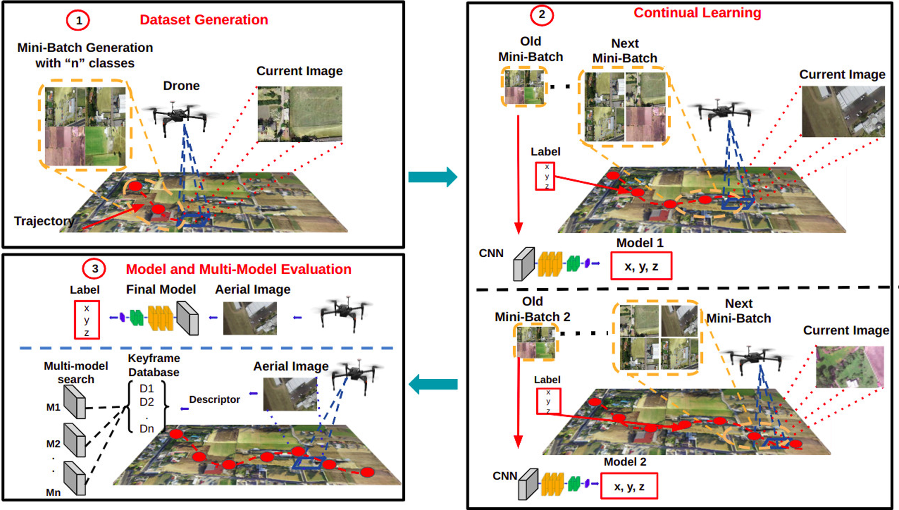
The continual learning approach consists of 3 steps: 1) Mini-batches generation during the UAV’s flight; 2) Continual training using previous mini-batches while new ones are created; 3) Model and multi-model evaluation to classify the current aerial image and get a flight coordinate in a sub-mapping fashion. We use a keyframe search based on a colour histogram to identify the corresponding model in a multi-model approach.
Our approach can be seen as a topological geo-localisation since the model will learn to predict the index of the mean flight coordinate of a single aerial image. Likewise, we propose a methodology for a sub-mapping-like approach using multiple models learned for each mini-batch rather than training a model for the whole trajectory. Finally, we argue that using mean flight coordinates helps localise the UAV and determine the flight’s course like an auxiliary localisation system.
To present our approach, the rest of this paper is organised as follows: Section 2 introduces continual learning approaches using images. Section 3 shows the methodology using the latent replay applied to a topological geo-localisation with aerial images and a multi-model implementation. The experimental design and comparison results are conveyed in Section 4, and the discussions about them are in Section 5. Finally, conclusions and future work are outlined in Section 6.
Camera localisation is an effective technique to estimate its poses in an environment using visual methods and image processing. In traditional visual positioning, features and the Nearest Neighbours method are used to get the localisation with matching strategies [11]. On the other hand, SLAM systems are popular methods used for robotics and navigations tasks [12], creating a map of the environment to obtain the camera poses and re-localise through bag-of-words (BOW) and Vision Fusion [13]. Besides, SLAM systems like ORB-SLAM2 [14] get a re-localisation using feature matching and BOW when the tracking is lost. At the same time, the work [15] presents a technique of rapid re-localisation for mobile robots, improving the ORB-SLAM2 system and adding an off-line map.
Some geo-localisation and navigation methods using agricultural robots in crop fields are based on satellite images and edge-matching to be localised [16]. Due to the impact of localisation systems, [17] suggests that retrieving a set of quality 2D-3D points can be used for re-localisation using a quick search that reduces the number of visual descriptors. Also, existing works like [18] propose a method using overlaps between frames to retrieve nearest pose neighbours with high accuracy. Likewise, the author in [19] presents a re-localisation approach that combines vision and CNN, improving the accuracy in regression to relocate mobile robots in indoor scenarios [20].
In the literature, we can find a wide variety of techniques for localisation based on deep learning. For example, the work in [7] proposes to use a PoseNet to predict GPS coordinates from a single image [21]. This CNN network uses a model training created from a single-image dataset to regress a camera pose associated with 3D or GPS coordinates. Furthermore, a study in [22] evaluates position accuracy and the processing speed in estimation networks against a compact network. Nevertheless, these works require collecting the dataset on a flight mission to train and test on another flight after the model is available.
Due to traditional learning methods, continual learning aims to perform online training on a CNN with small batches of incoming data without forgetting the previous ones. The latter was addressed by [23], which presents an architectural strategy called Elastic Weight Consolidation (EWC) to learn handwritten digits incrementally. In addition, Deep Neural Networks (DNNs) play an important role in batch learning settings, reducing errors and updating the model’s parameters [24]. Likewise, [25] uses a Hedge Backpropagation (HBP) method for updating the model parameters, as well as in [26] that uses a multi-layer LSTM as input for the same purpose.
Another group of techniques uses shared networks to pass the parameters throughout the architecture and learn incrementally [27]. Other methods include distillation, where a model incrementally learns new tasks while sharing the knowledge and updating its parameters [28]. Furthermore, Less Forgetting Learning [29] and Learning without Forgetting [30] focus on keeping the decision boundary unchanged, whereas the latest targets are updated. On the other hand, some examples are applied to specific vision tasks like object recognition using rehearsal strategies that allow replaying the old data and learning new ones [31, 32]. Finally, [9] presents a method based on MobileNet with latent layers to store activations instead of a portion of data, learning new classes and accelerating the performance and the training of the CNN.
In this context, continual learning for localisation has been studied for new developments such as [33] that use the latent replay method for a multi-camera localisation approach. Furthermore, some use continual learning in combination with SLAM systems for sequential deployments in different environments [34, 35]. Finally, IMAP [36] is a work for 3D representations with a neural network and SLAM system applying continual learning to fill data in previously unseen places. Nonetheless, it is unsuitable for long scenarios due to the limited memory buffer, making it difficult to recover the location in long trajectories.
Motivated by these works, we decided to use CL for UAV geo-localisation in outdoor scenarios using a CNN that is being trained on the fly from new streaming data. We also built a frame search based on histogram colour and keyframes to identify the corresponding model to a part of the flight trajectory, reducing the time and speed performance computational.
Methodology
Our continual learning approach aims to get flight coordinates from a single aerial image using a latent replay method presented in [9]. We adapted this method to learn from aerial images related to flight coordinates, training thus during the flight mission and making the learned model available. Besides, we carry out a multi-model continual learning framework to indicate which model corresponds with the image to evaluate using a colour histogram and keyframe searching.
Dataset generation
We collected aerial images with GPS information using the Robotic Operating System (ROS) for software management between the UAV and our Ground Control Station (GCS). The aerial images were captured with a Zenmuse X3 camera onboard the Matrice 100 with GPS coordinates and altitude converted to metres. Thus, we carried out 4 flight missions to obtain the dataset where a pilot flew the UAV manually, acquiring the images to 128 × 128. The images depend on each trajectory, having between 600 to 7800 to train and 300 to 650 to validate. Note that with the use of continual learning, do not matter whether the amount of data is balanced. This is an advantage for continual learning since it works with little data to create a fast learning model, avoiding underfitting and overfitting in the training step.
We used the method in [37] based on featured matching to automatically select these images in the aerial image sequence under this criteria. Thus, we selected the images based on an amount of coincidence in terms of visual information w.r.t. other images, for instance, could coincide in 80% of the visual content, and we applied a data augmentation for each class. We refer to a class as a group of images captured with GPS coordinates in a part of the UAV’s trajectory. Thus, we calculate the mean of the coordinates to establish it as a label and save it in a text file where the network will learn the indexes associated with the classes and the aerial images. Finally, we show dataset examples in Fig. 2, corresponding to Areas 1, 2, 3 and 4, shown in the first, second, third and fourth rows. In addition, for a better understanding of the labels and the indexes, we offer the information in Tables 1, 2, 3 and 4.

Examples of the training dataset: Each row contains examples of images representing each of the flight areas. This dataset is available at link.
Distribution of classes’ index associated with 9 labels as discrete GPS coordinates for Area 1
Distribution of classes’ index associated with 7 labels as discrete GPS coordinates for Area 2
Distribution of classes’ index associated with 14 labels as discrete GPS coordinates for Area 3
Distribution of classes’ index associated with 26 labels as discrete GPS coordinates for Area 4
In Fig. 3, we obtained the coordinates in Google Maps from the trajectories in blue waypoints. Each waypoint represents the point where we collected the aerial images with the label expressed in latitude and longitude; red and green waypoints consist of the start and end of the trajectory. Finally, Fig. 4 shows the paths travelled by the UAV for each of the four areas. We depicted the training dataset trajectory in red for each flight and the testing dataset in green. Red and green squares indicate flight coordinates, and yellow circles correspond to the mean flight coordinate.
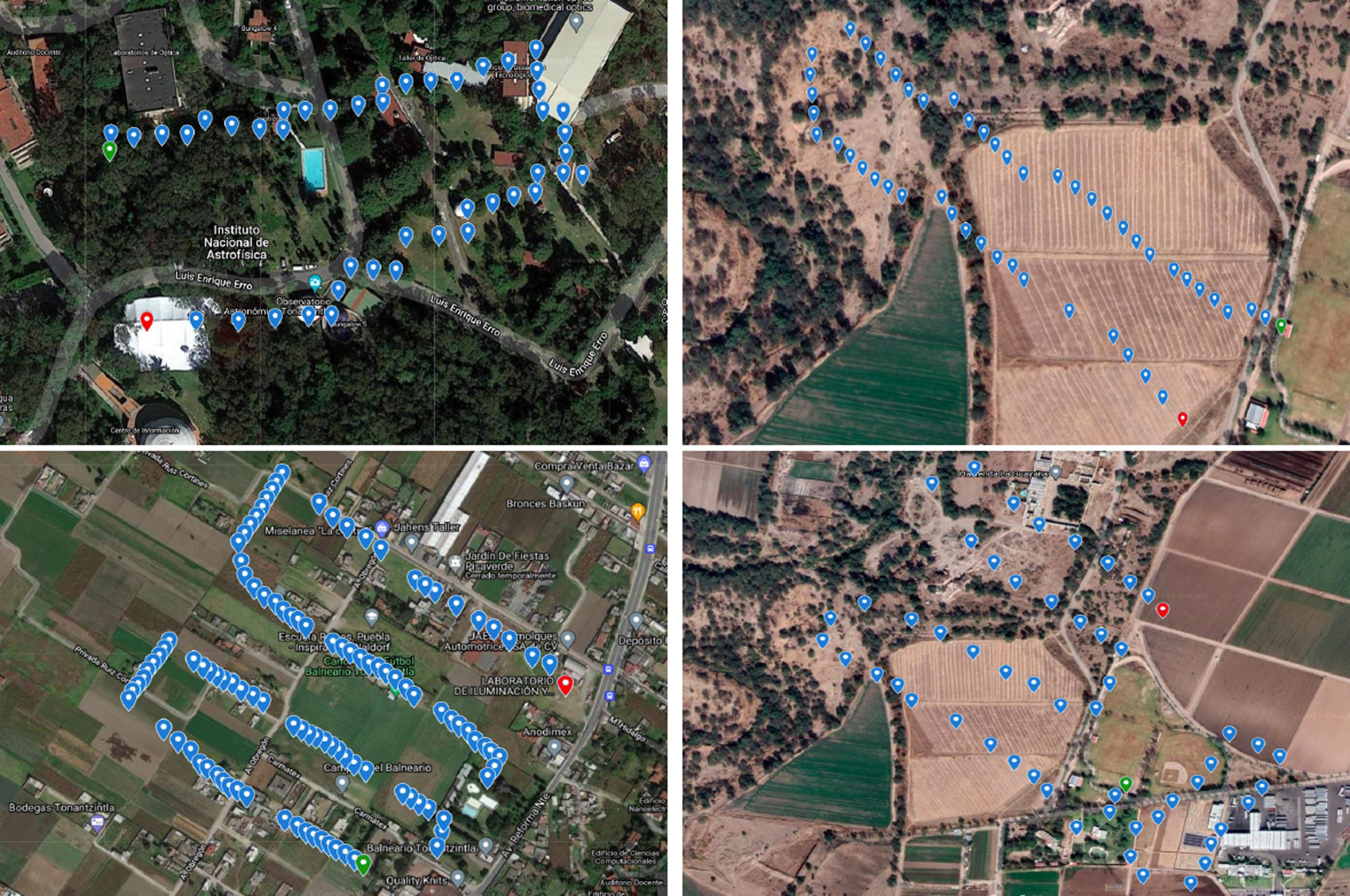
Trajectories into Google Maps where each waypoint consists of a GPS coordinate. The red waypoint represents the start of the path, and the green waypoint is the end.
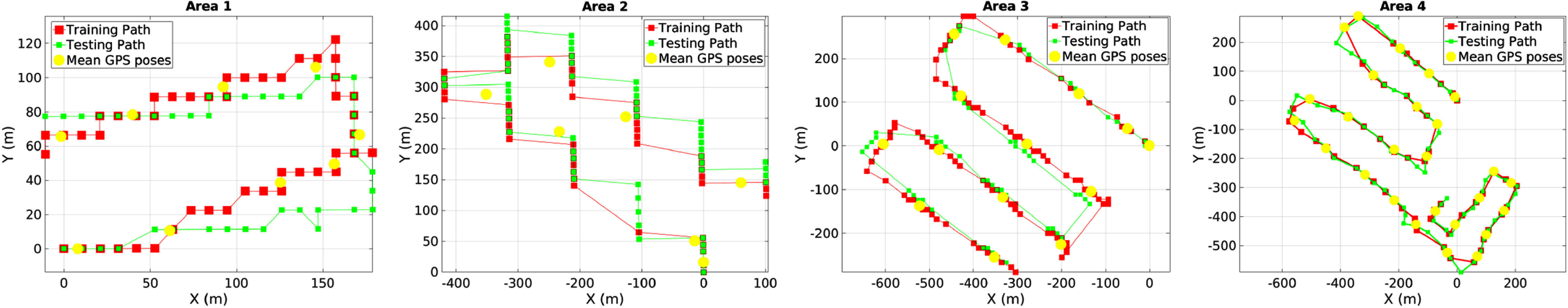
Mean GPS coordinates for each area where the total trajectory length flown by the UAV is as follows a) 1 km; b) 3.0 km; c) 4.6 km; d) 6.4 km. These trajectories include the training and evaluation path, both performed in the same flight.
The latent replay is an efficient technique for continual learning of new classes and new instances of known tasks from mini-batches. The process involves storing a portion of activations volumes at some intermediate layer, allowing slow-down learning at the layers below and leaving the layers above free. This increases the performance speed and reduces the training time compared to traditional learning methods. Hence, we proposed to slow down the learning at all the layers below the pooling6 layer, saving a small fraction of patterns for each class. In this manner, when the training is slow, an external memory rejuvenates the previous patterns to update with the new ones obtained from the following classes. Thus, we merge incoming patterns in the input layer with activations in the external memory.
We opted for using the same protocol and hyper-parameters introduced in [9] and the rehearsal memory of 1500 patterns for the first training. Then, we apply the continual training with 9 classes for area 1, 7 classes for the second, 14 for the third, and 26 for the largest trajectory in Area 4. Besides, each class contains 124 aerial images for Area 1, 92 images for Area 2, 40 for Area 3 and 301 for Area 4. We also apply data augmentation to increase the number of examples to train. Table 5 shows the total number of images for training (before data augmentation), the number of images used for validation (acquired during the return flight) and the number of mini-batches generated.
Datasets per area include training and validation sets, the number of classes, and the number of mini-batches. Each mini-batch can have data of 2 to 4 different classes.
Datasets per area include training and validation sets, the number of classes, and the number of mini-batches. Each mini-batch can have data of 2 to 4 different classes.
To show the latent replay method efficacy for a geo-localisation from a single aerial image, we propose increasing the number of patterns for storage and the epoch number shown in Table 6. Thus, we generated three models by varying the number of epochs and the number of patterns in the rehearsal memory. In addition, other training parameters are set to 1) SGD Optimiser; 2) Batch size: 128; 3) Epochs: 4 to 10; 4) Cross-Entropy as loss function; and 5) Learning Rate: 0.001.
Amount of patterns and epochs used to train three different models
We increased the number of patterns stored in external memory in the latent replay layer, which could improve the accuracy of training models. Nevertheless, the training updates the weights in the model when new data arrives, generating a single model with all the information learned and avoiding forgetting the previous data. To take advantage of the fact that each mini-batch updates the model, we propose generating a model for each small dataset in a multi-model approach, enhancing the accuracy of the final result rather than using a single one.
As indicated at the end of the previous session, we propose using a multi-model approach corresponding to each part of the trajectory. To do this, we create a search engine that allows us to choose the model for the evaluation using a simple descriptor based on a colour histogram of the images. Besides, we changed the network’s output to deliver a model per each mini-batch, thus having a model with information of 2 or 4 classes depending on the dataset. We also created a set of keyframes per trajectory, where each keyframe selected is the intermediate image between classes in a mini-batch. That is, the last image of a class is also the first image of the set of images of the next class.
For the search engine, we compute a histogram from the colour distribution in the image. Firstly, we convert the image colour space from RGB to HSV to improve the robustness of the histogram. Then, we define eight bins for the Hue channel, 12 for saturation and three for value. The total feature dimension vector is 8 × 12 × 3 =288. Then, we calculate a mask from a patch of 64 × 64 pixels placed at the centre of the image and coinciding with the four corners of the image, getting five regions to compute the histogram. Finally, we concatenated the five histograms to a vector of 1440 values between 0 and 255, representing the colour descriptor.
To find the model corresponding to a current image, we compute the histogram of the query image and the keyframes associated with each model. Then, we use the χ2 distance to compare the histograms [38] where a value closer to zero represents more similarity. Once the keyframe with the best match is found, we load the model associated with this keyframe for the evaluation step. A diagram to load the corresponding model is depicted in Fig. 5.
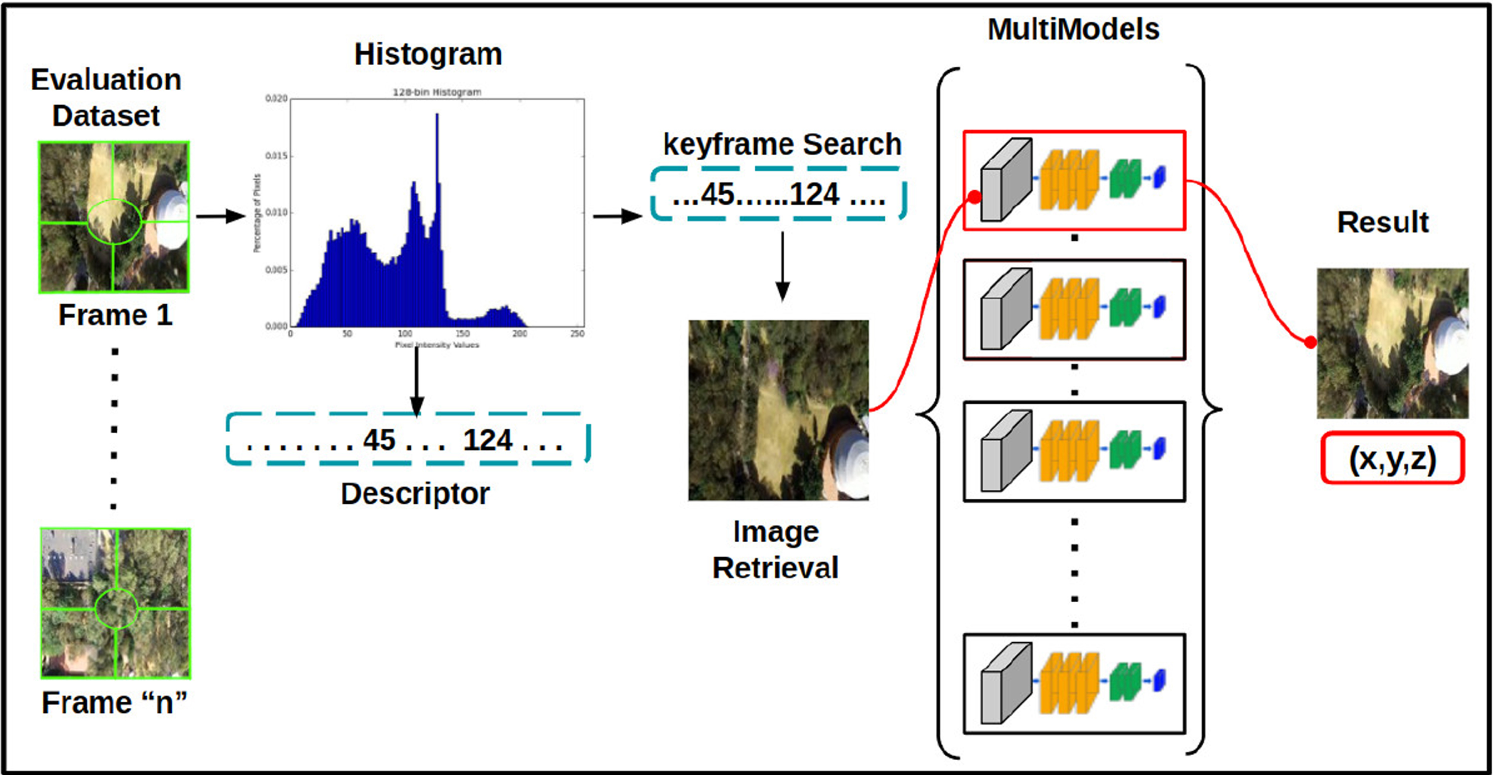
Overview: Keyframe searching with a current aerial image using the descriptor to identify the corresponding model.
This section shows the experiments and results obtained with the topological geo-localisation system using the latent replay method and aerial images. The experimental framework was carried out on Ubuntu 20.04, using PyTorch 1.4.0, Opencv 3, and Nvidia Geforce 960M, where all the processes ran on ROS. Firstly, we evaluated the three training models presented in the methodology to classify the images of each area. Then, we compare the accuracy obtained with the ORB-SLAM2 re-localisation module, the three models of the first experiment, the multi-model approach, and the EWC method adapted to the PoseNet architecture. Also, we show each method’s processing speed expressed in frames per second (fps).
In the first experiment, we tested the efficiency and accuracy of the three models using different training parameters with their respective testing datasets. These datasets correspond to aerial images acquired during a return home trajectory, i.e. when the UAV flies its way back home. The accuracy results are shown in Table 7, indicating that model 2 maintains better accuracy of the previous classes’ patterns without forgetting them in areas 1 and 2, model 3 achieves a better result than the others in area 3, and model 1 in area 4. In this way, we can use the best model to re-localise the UAV using only the aerial imagery associated with the mean flight coordinate. In this way, model 2 has a better performance whose training parameters offer fast mission-ready learning, using fewer data than traditional learning methods.
Accuracy result using the test dataset. The best results are highlighted in bold
Accuracy result using the test dataset. The best results are highlighted in bold
On the other hand, we argue that having a mission-ready learning model is an advantage for a localisation task in which a UAV loses its GPS signal, using this approach like an emergency return home system. To show the model’s performance regarding the flight coordinate estimation during the evaluation trajectory, we present an illustrating video of geo-localisation in trajectories 3 and 4 . Also, we show in Table 8 the traversed trajectory length of flight for each area expressed in km.
Traversed flight trajectory length for each area
Hereafter, we present the second experiment to compare the accuracy and processing speed results with a single learning model, a multi-model approach, ORB-SLAM2 and EWC. For a multi-model process, a search engine for a keyframe using a descriptor based on the colour histogram of the image is essential to establish the chosen model. Also, for the EWC approach [23], we adapt this strategy using PoseNet architecture based on the regularisation of weights to avoid catastrophic forgetting. Thus, this strategy uses policies that regulate the transfer of weight parameters and avoid overfitting the new information and forgetting previous knowledge.
The EWC slows down the learning of weights using a penalty applied to the parameters of a layer, a kernel, bias or optimisation functions. Therefore, this penalty optimises the network parameters giving a probability of the information approximating the previous distribution. Finally, we also compared the re-localisation method of a robust state-of-the-art visual SLAM system known as ORB-SLAM2 [14]. ORB-SLAM2 uses its re-localisation module when tracking is lost, recovering the camera’s position in the environment using feature matching and binary descriptor correspondences with the image. To get the re-localisation with the ORB-SLAM2 module, we performed the following steps:
We use the training dataset to make the map in the SLAM system. In this sense, we create and store ORB descriptors and the map for future re-localisations when the tracking is lost. We use the evaluation dataset to call the ORB-SLAM2 re-localisation module to get the flight coordinates and re-localise the camera into a scenario. Finally, we store the poses in a file text for future analysis. We use the evaluation dataset and activate the mapping to continue to create the map. In this way, we get the position of the evaluation dataset and compare this result with the re-localisation module given to us. Finally, we evaluate the ORB-SLAM2 localisation module using a threshold between the positions of the mean coordinates. This threshold represents the distance between classes, so if an image is re-localised in its respective class threshold, it is taken as a valid result; otherwise, it is incorrect.
Using the above approaches, we show a comparison in Table 9, obtaining a lower accuracy with the EWC method and the ORB-SLAM2 w.r.t our results using a single model or multi-model in Area 1. We attribute this to the fact that ORB-SLAM2’s re-localisation is affected by descriptor mismatching due to rotation and illumination changes that vary from the training images. Although for trajectories 2 and 3, ORB-SLAM2 improved its performance, having a similar result to our single and multiple model approach.
Accuracy results over the four trajectories using the Models, EWC, ORB-SLAM2 re-localisation module, and multi-model approach
Accuracy results over the four trajectories using the Models, EWC, ORB-SLAM2 re-localisation module, and multi-model approach
It is worth noting that some of the similarities of our work with ORB-SLAM2 are the type of descriptor search to establish the re-localisation. While ORB-SLAM2 does this with a BoW and feature matching between a query image and keyframe, we search the histogram colour using the χ2 distance between a query image and a keyframe, allowing find and load a model corresponding to the part of the trajectory. On the other hand, the main difference is that ORB-SLAM2 obtains the camera pose through similar descriptors between the current image and the keyframe within the map. And we get the camera pose using the model’s classification, thus giving the mean flight coordinate.
Note that EWC fails in Areas 2 to 4, meaning that the method needs to learn more information to solve the task, thus returning incorrect values only. However, our approach works better than ORB-SLAM2 in Areas 3 and 4. Furthermore, ORB-SLAM2 requires the camera’s calibration to perform the re-localisation, whereas our method does not.
In Table 10, we show the processing speed expressed in fps for all the methods evaluated in this work. In this regard, our multi-model method outperforms all the other approaches with better accuracy, encouraging the development of continual learning methods for real-time re-localisation with a multi-model system. Finally, to better understand the results obtained, we present in Table 11 the RMSE metric to observe how far the obtained values are from the ground truth. In this way, a minimum value represents a better fit to the accuracy measure with which the algorithm performs the evaluations, getting a better performance for the multi-model approach.
Fps results over the test trajectories using Model 1, 2, 3, EWC, ORB-SLAM2, and multi-model approach
Comparison results using the RMSE metric
To better understand, we discussed the results regarding complexity and training time with the comparison works. Firstly, for training time, our work has a time between 40.4 to 48.7 sec per mini-batch, in contrast to traditional training, which can take much longer. For the EWC method, the training time using the PoseNet architecture is around 57.4 to 86.5 sec per mini-batch. Nonetheless, the accuracy is lower than our work, so if we trained with a larger dataset, its accuracy and training time increased, but this is not the purpose of the comparison. Besides, we would need to create the dataset previously and not in the same flight mission.
On the one hand, in terms of complexity, we observed that SLAM systems rely on storing and updating the descriptors within the map at each time step [39]. Under the assumption that the whole map needs to be updated, the operations require a complexity approximate of O(n3) for n cameras [40]. On the other hand, the complexity of the architecture of deep learning is linked to the expressiveness or representability of the limit of a model, thus measuring the degree of fit of random noise in a hypothesis space. According to work [41], the complexity of a deep learning network is the Rademacher complexity [42]. This mentions that the complexity of deep learning architectures varies depending on the size of the data, the depth, its optimisation process, and the size of the model itself.
Given this analysis, the complexity depends on its parameterisation in the learning models, having an estimated train-time complexity of O(p2× (n+p)) for regression architectures such as PoseNet, even with the EWC method. While for a classification model, its train-time complexity is around O(np) where n is the number of observations and p are the number of predictors or features.
Overall, our approach has an average training time of 44.5 sec upper to the EWC method with PoseNet, and a train-time complexity of Rademacher. In addition, we do not need to create a map of the place, neither to calibrate the UAV camera nor to have a dataset a priori to carry out the geo-localisation of the flight mission.
Finally, we present a qualitative comparison of the geo-localisation obtained by our approach and the ORB-SLAM2 module. In Fig. 6 and Fig. 7, we can appreciate the results obtained from trajectories, where the training trajectory is highlighted in red, the testing trajectory in green and the yellow circles represent the classes. Likewise, if an image is correctly localised, it is linked to the corresponding class with a blue line; otherwise, we mark it in black. In Fig. 8, we show the re-localisation obtained with ORB-SLAM2 in green circles corresponding to aerial images re-localised. Nonetheless, in some parts of the testing trajectory, ORB-SLAM2 does not achieve localisation (e.g., in Area 1, just ten images are localised correctly). We argue that this is for the lack of features in the mapping that do not correspond to the image, giving a wrong location or even no localisation.
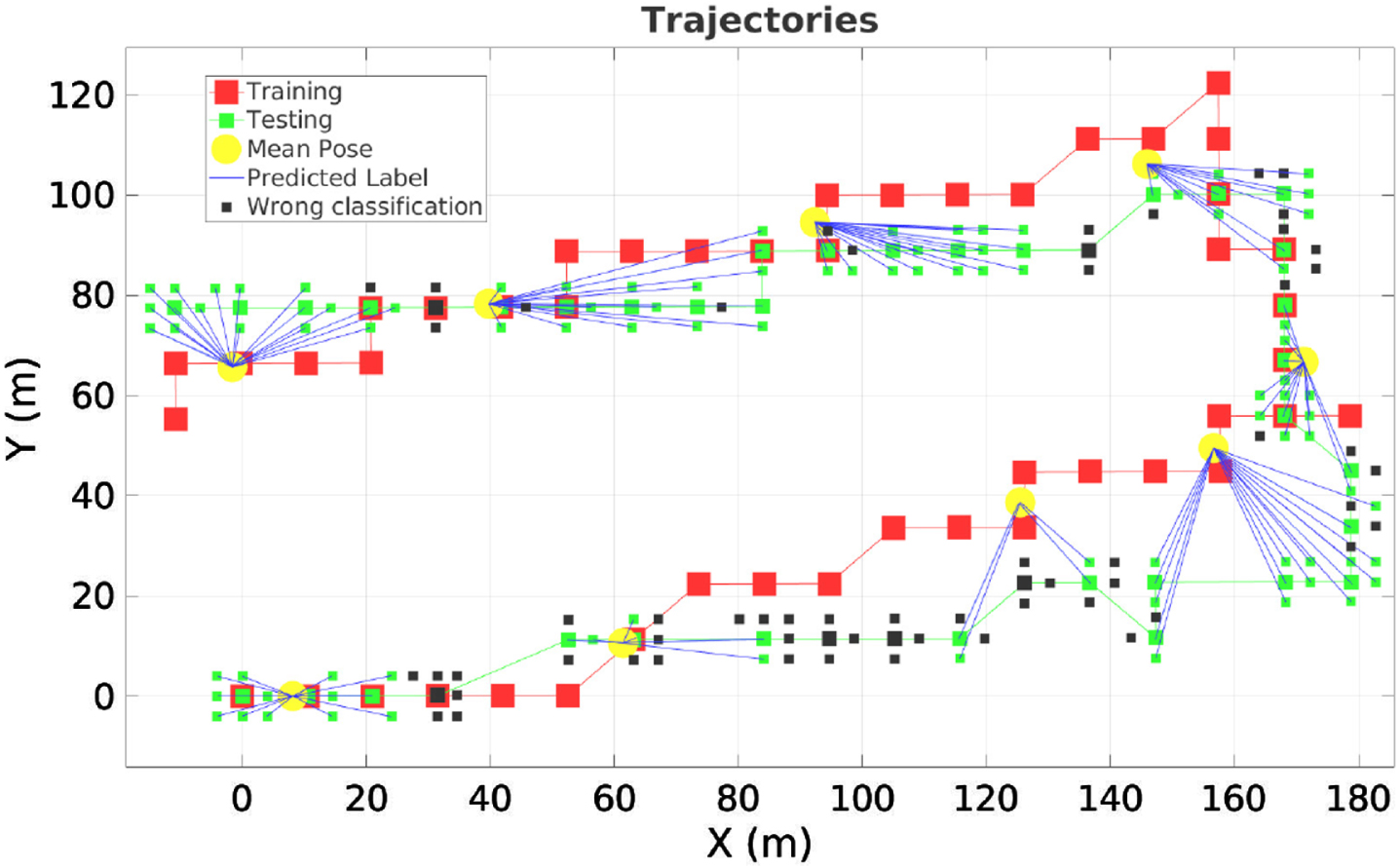
Geo-localisation using our approach to Area 1. Incorrect classifications are shown in black and correct in green with a blue line towards the class.
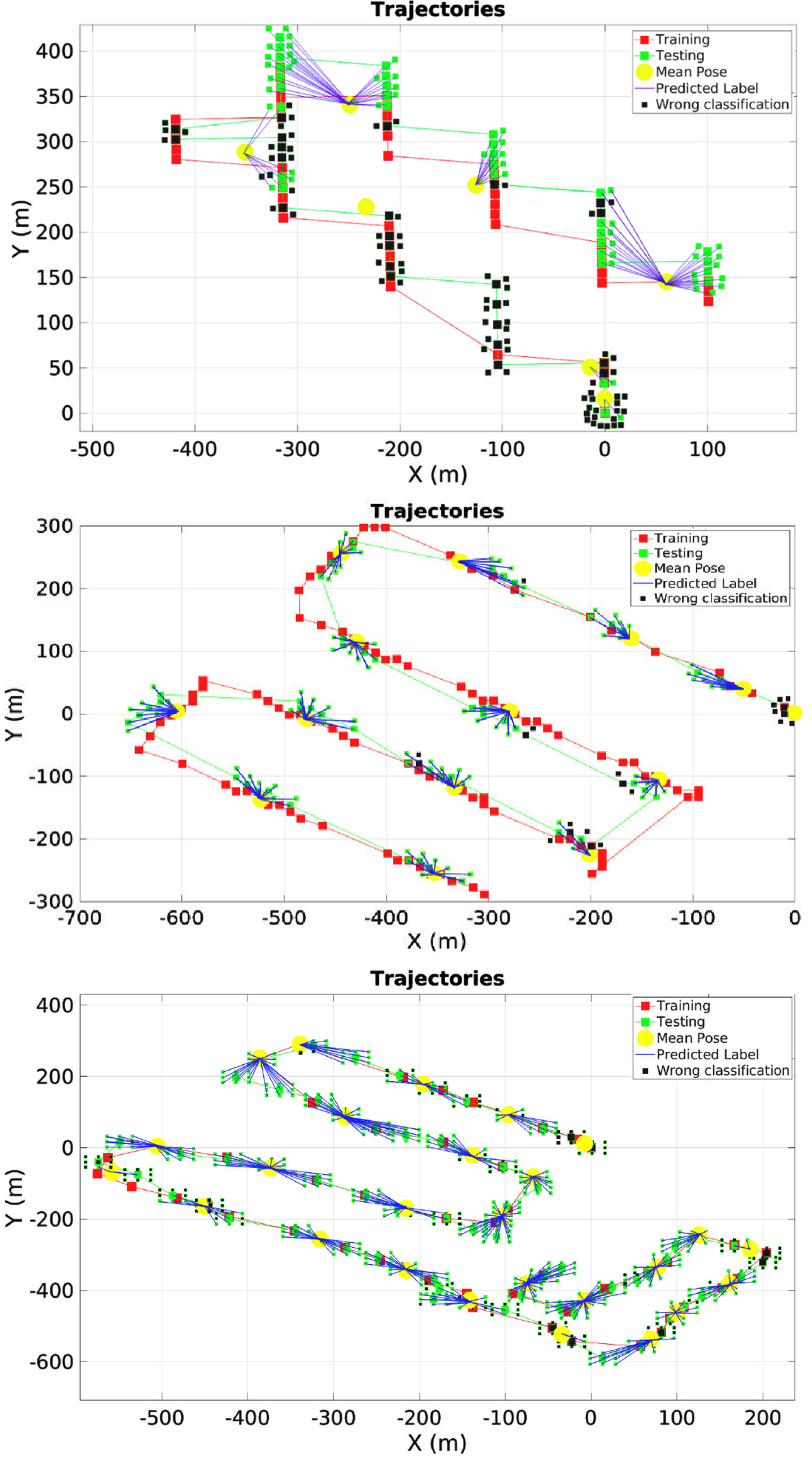
Geo-localisation using our approach into Areas 2, 3, and 4. Incorrect classifications are shown in black and correct in green with a blue line towards the class.
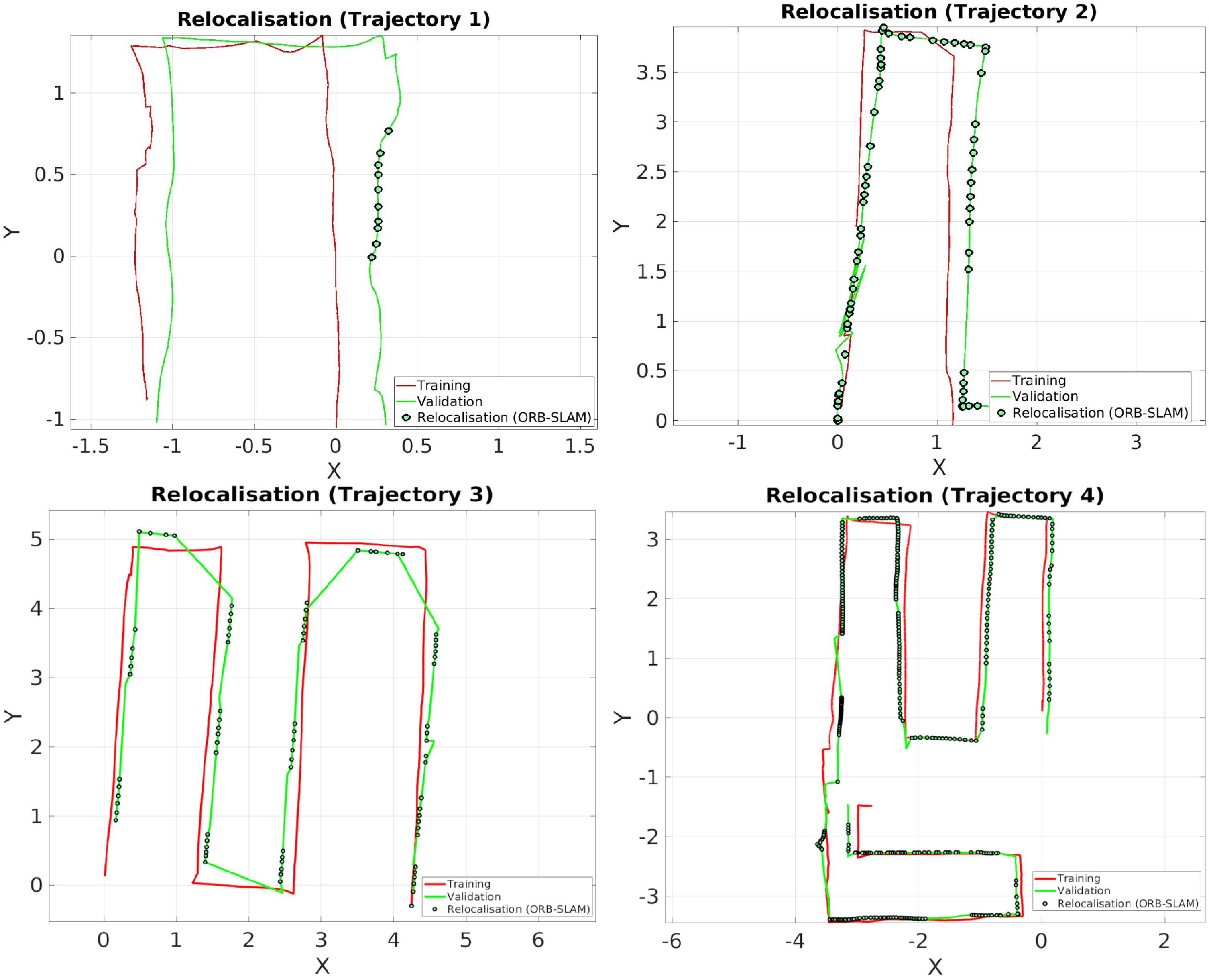
Re-localisation using ORB-SLAM2. We indicate the training trajectory in red and the validation trajectory in green. The correct localisation is present in green circles.
We have presented a continual learning approach to address the problem of geo-localisation from a single image and a multi-model camera localisation using a keyframe search, thus seeking to extend the former methodology in a sub-mapping fashion. Furthermore, we have explored a continual learning technique based on a rehearsal strategy using a latent replay method to train data with a sequence of aerial images. The advantage of this method is that of being able to increase the model’s knowledge from new instances without forgetting the old ones using a latent layer to store the classes’ patterns.
We have evaluated our proposed methodology with different real-world flight trajectories. On average, the accuracy result of the best model is around 0.75 with a processing speed of 111 fps. These results encourage the development of robust aerial systems capable of learning a model online that associates aerial images with GPS information, which could be helpful in the case of GPS failure during a flight mission.
Likewise, our multiple models learned with continual learning exhibits a better performance than using a single continual model in terms of accuracy. We attribute the latter to the fact that the multiple models are kept compact with less information that could clarify the model inference. Overall, this approach achieves an average accuracy result of 0.77 while maintaining a fast processing speed of 150 fps.
Our geo-localisation method based on latent replay is currently limited to 1000 classes to be learned. Thus, in our future work, we will investigate new strategies to overcome this limit, including regressing aerial images directly to GPS coordinates. Regarding the multiple model module, we will investigate a more sophisticated image search engine to find the best image associated with the corresponding model.
Acknowledgments
The first author is thankful for his scholarship funded by Consejo Nacional de Ciencia y Tecnologia (CONACYT) under grant 802791.