Forecasting cholera disease using SARIMA and LSTM models with discrete wavelet transform as feature selection

Abstract

Throughout history, cholera has posed a public health risk, impacting vulnerable populations living in areas with contaminated water and poor sanitation. Many studies have found a high correlation between the occurrence of cholera and environmental issues such as geographical location and climate change. Developing a cholera forecasting model might be possible if a relationship exists between the cholera epidemic and meteorological elements. Given the auto-regressive character of cholera as well as its seasonal patterns, a seasonal-auto-regressive-integrated-moving-average (SARIMA) model was utilized for time-series study from 2017 to 2022 cholera datasets obtained from the NCDC. Cholera incidence correlates positively to humidity, precipitation, minimum temperature, and maximum temperature with r = 0.1045, r = 0.0175, r = 0.0666, and r = 0.0182 respectively. Improving a SARIMA model, autoregressive integrated moving average (ARIMA), and Long short-term memory (LSTM) with the k-means clustering and discrete wavelet transform (DWT) for feature selection, the improved model is known as MODIFIED SARIMA Outperforms the LSTM, ARIMA, and SARIMA and also outperformed both the modified LSTM and ARIMA with an RSS = 0.502 and an accuracy = 97%.

Keywords

Cholera forecasting SARIMA K-means clustering discrete wavelet transform

1 Introduction

Cholera, which is caused by the microorganisms Vibrio cholerae 01 or 0139, manifests as watery diarrhea and severe intestinal illness [1–3]. The exotoxin produced by Vibrio can cause serious symptoms such as electrolyte imbalance, dehydration, and circulatory failure [4]. If the chain reaction is allowed to continue without appropriate medical intervention, consequences like myocarditis, acidosis, tubular necrosis, heart failure, and death may occur [5].

The fecal-oral pathway is the most prevalent way for cholera to spread, and it is brought on by tainted food and beverages caused by a lack of basic hygiene [1, 6]. In developed nations, consuming contaminated food is the main means of cholera infection transmission. On the other hand, cholera is typically spread through contaminated water in undeveloped countries [7].

Worldwide, 28 to 150 thousand cholera deaths and 3 to 5 million cholera illnesses are estimated and recorded each year. Yet, the occurrence is more common in undeveloped countries with significant levels of human poverty in the tropical and subtropical areas [2, 8]. The authors in [3] claims that there have been seven cholera pandemics since 1817, with the seventh pandemic causing the majority of the world’s infections. In the majority of African countries, cholera has spread to be an endemic illness in less than five years [9].

In 2012, 86% of cholera deaths and 71% of all reported cases were found in Sub-Saharan Africa [5]. Although 129,064 cases and 2102 deaths were reported in 2013 by 47 nations, the World Health Organization (WHO) indicated that the exact disease epidemic is just 5–10% of the cases that are officially reported. The disparity between reported data and the estimated illness burden might be attributed to inadequate monitoring and laboratory systems. A total of 52812 (83%) of the 63658 cholera deaths documented by the WHO between 2000 and 2015 were in sub-Saharan Africa, but this figure is likely an underestimate. The number of nations reporting indigenous cases of cholera has increased from 24 in 1971 to 30 in 1998 and 36 in 2008, and decreased to 27 in 2011 [6, 10, 11]. Sub-Saharan Africa accounted for 1,080,778 of the 4,426,844 (24%) cholera cases reported to the WHO between 2010 and 2019 from 34 countries [12, 13].

The first cholera cases in Nigeria were discovered in a community close to Lagos State in 1970, with an unknown total of cases and a case fatality rate (CFR) [14]. This outbreak resulted in 22,931 cases, 2,945 fatalities, and a CFR of 12.8% in a population of 1,477,000 in 1971 [15]. The latest 2018 cholera epidemic in Nigeria, which resulted in over 45,000 cases and a 1.9% CFR, shows the country’s high cholera burden [15].

Furthermore, except for Liberia, which reported just two cases, it was only Nigeria that recorded cholera cases in 2021 in the West African sub-region, with 93,362 cholera incidents reported and 3,283 cholera-related deaths resulting in a CFR of 3.5%; 32% of the Federal Capital Territory (FCT) had the most cholera cases [16]. In line with global epidemiology, the primary indicators of cholera spread is the unavailability of clean drinking water and unhygienic situations [17]. Several variables are potential aids in the transmission of cholera in Nigeria, including lack of safe drinking water, unclean surroundings, natural disasters, illiteracy, and internal conflicts that cause people to flee to internally displaced people (IDP) camps [18].

Water is likely a major factor in cholera epidemics in Africa [19]. Floods, which are caused mainly by high rainfall, enhance the spread of water-borne illnesses by hindering access to safe drinking water, contaminating safe water sources, causing sanitary issues, and restricting access to essential health services [20]. Water becomes easily contaminated during and after rains due to the washing of open-air defecation grounds or spills from pit toilets, both of which contribute to a worsening of sanitary conditions and an increased risk of cholera transmission. It is also observed another contributing reason has been discovered: a lack of efficient sewage disposal, because of the contamination of the food and water in the area from individuals buying and selling food close to trash bins, the cholera pandemic may happen if people ingest contaminated food and water [3].

Another enabling factor that enhances cholera transmission is increasing the pressure on already congested sanitation facilities; a densely populated area with informal and low-quality housing also impacts cholera occurrence and epidemic intensification. In Harare, cholera attack rates in 2008–2009 varied from 1.2 cases per 1,000 persons in a less dense residential areas to 90.3 cases per 1,000 in an overpopulated environs, with Ghana and Uganda showing similar trends [1]. According to a research in Kenya and Yemen, rising violent conflicts can have a global impact on recurrent cholera transmission [21].

Climate conditions, particularly tropical rain, have a well-established relationship with cholera outbreaks as significant climatic elements that aid to the spread of cholera in Nigeria [22]. According to [22], the Southern Oscillation Index (SOI) and Sea Surface Temperature (SST) also aid in the spread of cholera in Africa. A detailed analysis of the relationship between cholera incidence and climate factors using various statistical techniques in various parts of the world has been done [23].

According to the review, there is a statistically significant correlation between the prevalence of cholera in different nations and climate factors including Nigeria’s average temperature, relative humidity and precipitation [22]; The authors used generalized additive modeling (GAM) and multiple linear regression (MLR) and found that the temperature and rainfall have a dynamics in the spread of cholera disease.

In another study conducted by [24], strong coherence was found between cholera epidemic resurgences in Ghana and climatic/environmental characteristics. After cross-correlation analysis, rainfall and SOI correlate with the number of cholera incidences. A strong correlation also exist between rainfall and cholera cases in Senegal after a Cross-correlation analysis [24].

In order to evaluate the relationship between the rise in number of incidence weekly and the mean of the daily maximum temperature and rainfall on a weekly basis, a Poisson autoregressive model for trend control was designed in Zambia, there has been a 2.5% rise in the number of cholera cases with a 50 mm rise in rain 3 weeks earlier and a 5.2% increase in cholera incidence with a 1 °C rise in temperature 6 weeks prior [25].

In addition, cholera cases increased 2 times with a 1°C temperature RISE and a 4-month delay, but only by 1.6 times with a 200 mm increase in rainfall and a 2-month delay. At a 1-month lag, Zanzibar’s temperature and rainfall increased, producing a positive association (P = 0.04) [26].

A Poisson regression model was employed in southeastern African nations to examine the probable relationship between cholera incidence rates and yearly variations of temperature and sea surface temperature (SST) [27]. During the research period, the results showed that cholera rates in individuals had significantly increased and the analysis of the annual average air temperature and the SST revealed a significant relationship between these variables and cholera occurrences [27].

The WHO-led Global Task Force on Cholera Control (GTFCC) released their “Roadmap to End Cholera by 2030” in 2017. Rapid response to outbreaks is a key part of the road map. This objective would be greatly facilitated by a low-cost, reliable rapid diagnostic test (RDT). There are a number of commercial RDTs that are being used for surveillance or during outbreaks. These tests are portable and suitable for almost any setting [28]. However, the accuracy and dependability of the tests that are currently available can vary depending on the user and the circumstances. Public health experts have been reluctant to declare an epidemic based only on the results of an RDT because they have little confidence in the existing cholera RDTs. This may lengthen the time it takes to respond to an outbreak [4, 29].

A form of artificial intelligence uses algorithms to find patterns in data called Machine Learning (ML), are used to create a data model that can make predictions that are more accurate [30]. Machine learning has been employed in a number of ways to predict, identify, and prevent the development of severe infectious disease epidemics [31]. In recent decades, there have been numerous research and significant advances in the development of commonly used models and methodologies for precise cholera prognosis and forecasting.

In Hanoi, three distinct forecasting models called the complete (CP), the weather-independent (WI), and the geographically independent (GI) were developed. The weather and prior cholera cases from the entire region are used as supplementary predictors for each model’s lagged parameter (l), measured in days. The RF regression technique was used to develop a machine learning (ML) model. With the CP model being the best model, the adj-R² measure was reduced with 0.0076, and the 95% confidence interval is [0.0095, 0.0057] if all other variables are held constant and the forecasting duration is increased by a day [32].

The author in [33] proposed a new method to enhance the accuracy of cholera cases prediction in Hanoi, Vietnam, by using solar terms, which is an ancient Chinese idea that signifies an exact point of season change in lunisolar calendars; and the training data being resampled. Results from the research validate the research, by combining solar nomenclature with random oversampling example and random forest obtaining an area under the curve (AUC)=0.84 and very strong sensitivity and specificity [33].

In order to predict the prevalence rate of the most recent cholera outbreaks in a Yemeni governorate, the authors in [34] proposed the cholera artificial learning model, which is made up of four (4) extreme gradient-boosting machine learning proto-types. Using previous cholera data, fatality rates, civil war casualties, and interconnections across governorates depicted over many years, CALM is a revolutionary ML approach.

In another research, the authors in [35] proposes ML methods the adaptive synthetic sampling approach (ADASYN) with principal component analysis (PCA) methods are used for dealing with the imbalanced dataset problem and restoring the dimensionality of the dataset’s sample balance. The researchers also compared other ML approaches and discovered that the XGBoost algorithm performed better than the RF classifier for predicting cholera cases in Tanzania, with a sensitivity of 0.805 and 0.645, respectively. The XGBoost was selected as the best model for the study on the basis of the model’s characteristics [35].

The cholera pandemic has been predicted in previous research using key climate factors from satellites, such as atmospheric, terrestrial, and oceanic data. The authors [36] used a novel approach to test if a machine learning system could predict an environmental cholera pandemic. 89.5% of outbreaks were classified by the RF classifier as having accuracy = 0.89, sensitivity = 0.89, and F1 scores = 0.942 [36].

The cholera forecast model employed simple stochastic time-series SARIMA. The temporal clustering of cholera at lags of 1 month and 12 months were detected by the SARIMA model. Their research indicates that a minimum temperature change of 100°C causes a 6% increase in cholera infections during this time of year. When the sea surface temperature (SST) rises by 10°C, cholera incidence increase by 18% and 25%, respectively, in the present month and after two months. Over the research period, rainfall had no impact on the incidence of cholera. The model did reasonably well in forecasting the variability in cholera cases, with a root mean square error (RMSE)=0.108. Therefore, the ambient and SST-based models can be utilized to forecast cholera epidemics [37].

A correlation between climatic factors and cholera cases was found in [23]. According to their research, the two factors that affect cholera prevalence the most are rainfall and maximum temperature. A cholera incidence time series study was conducted from 2000 to 2013 using a SARIMA technique because of the auto-regressive and the seasonal behavioral pattern of the illness. Models A, B, C, and D were created as single variables SARIMA models (SVM) and multiple variables SARIMA models (MVM). These models were then compared and their relationship to cholera outbreaks was assessed. An Akaike information criterion (AIC)=21 and Bayesian information criterion (BIC)=39 was obtained, where the MVM outperformed the SVM with RMSE = 16.2 and MAE = 13.2, with RMSE = 14.7 and Mean Absolute Error (MAE)=11, respectively. In addition, it had BIC = 36 and AIC = 15.

The method’s drawback is that feature extraction and selection were not used, which is thought to increase the accuracy of the outcome and bring the error rate of the model down to a minimum [23]. In order to use SARIMA for cholera forecasting, the proposed research will thus employ a unique method that combines the DWT as a feature selection method and outlier detection using the K-means clustering. The aim of this research was to develop a Modified SARIMA model with the following objectives:

To determine whether incorporating DWT will improve the performance of the model?

To determine whether the detection and removal of outliers in the data using K-means clustering will have an effect on the performance of the model?

Establishing a link between cholera incidence and climate factors.

To compare different time series models and select the best fit.

2 Materials and methods

DWT and time series forecasting were used to build the proposed model. According to [38], DWT can quickly identify abrupt signal changes and minimizes noise as well as reducing the size of the data and its dimensionality. The modified SARIMA, ARIMA, and LSTM models were built after applying the feature extraction in order to narrow the selection so that only relevant features were used before the outcome are analyzed and evaluated.

2.1 Data collection

The dataset utilized and its source are described in this section. The dataset used in this study is a cross-sectional data set that spans the months of January 2017 and May 2022 and contains monthly cholera cases and climatic factors.

2.1.1 Cholera cases

The weekly epidemiological reports made accessible to the public in portable document format (PDF) from January 2017 to May 2022 obtained from the Nigerian Center for Disease Control (NCDC) contained information on cholera outbreaks at the state level in Nigeria. Each report offers thorough details on the illness including the states, the number of cases recorded, CFR, number of deaths, culture, and rapid diagnostic test (RDT). Over the years 2017 through 2021, there were 172135 reported cases in total, with 2021 having the most cases. A Microsoft Excel (.xls) file was created from the whole dataset. Figure 1 shows the reported cholera cases to the NCDC.

Fig. 1

Time series pot for reported cholera cases.

2.1.2 Weather variables

The source of all climatic data is the European Center for Medium-Range Weather Forecasting (ECMWF). The systems’ resolution ranges from 0.1 to 0.25, and it has over 1.8 temperature billion data points. Data on precipitation, temperature, humidity, and Sun hours were collected for many countries between 1991 and 2021 using daily, weekly, monthly, and yearly records which are calculated for each state in Nigeria as well as the Federal Capital Territory (FCT) using the monthly average for each state. In Figs. 2–4, the maximum monthly average temperature (0°C), total accumulated rainfall (mm), and relative humidity (%) are all displayed.

Fig. 2

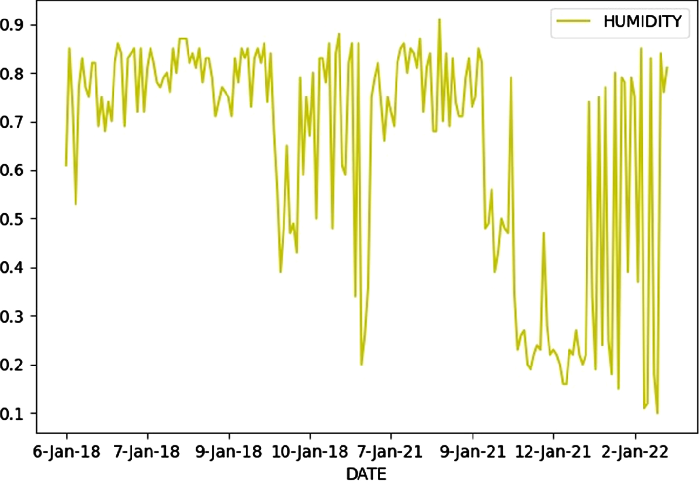
Time series plot relative humidity (%).

Fig. 3

Time series plot maximum temperature (°C).

Fig. 4

Time series plot for minimum temperature (°C).

2.2 System implementation

Anaconda 3, an open-source program that is compatible with Python 3.8 was used to implement the proposed model (Modified SARIMA) on a Windows 8 PC with 16 GB RAM and a core i5 CPU. The steps were used in building the forecasting model are discussed in the subsections below.

2.2.1 Data preprocessing

It the process of cleaning, incorporating, choosing, modifying, normalizing, and extracting features [39]. Everyday data is typically inadequate, unclean, inconsistent, and untrustworthy. The efficacy, correctness and accuracy are boosted if any data irregularities are identified, repaired, and rectified at an initial stage of data pre-processing, which result in a very effective and reliable decision-making process. Data quality is vital for ML-based sickness prediction. To improve the usability and application of the first dataset for cholera forecasting, the two data acquired were integrated, and multiple preprocessing procedures were used.

2.2.2 Feature extraction using DWT

Feature extraction is defined as process of generating a significant sets of attributes from real time-series dataset and removing unnecessary variables. Feature vectors are another name for this collection of features [40].

Because DWT samples’ wavelets are at distinct intervals, it is often used for feature extraction and functions as an effective feature extractor [41]. Simply by discretizing the scaling variables logarithmically and coupling them to the step size implemented between the translational variable values (t), the insertion of discrete scale and translation variables values during wavelet transformation enable it to reduce the redundant signal data [42]. This exhibits how hidden frequencies can be processed to produce extremely distinctive, useful attribute for classification, regression, pattern recognition, and other ML algorithms that evaluates discrete signal time frequency. The method also approximates and details original signals using low- and high-frequency filters [43]. Equation (1) defines DWT using wavelets and scaling for a certain k-level DWT function and an f(r) signal.

$\begin{matrix} f (r) = \sum_{n} b_{J} (n) φ (r - n) \\ + \sum_{n} \sum_{j = 0}^{j - 1} c_{j} (n) 2^{j / 2} Ψ (2^{j} r - n) \end{matrix}$ (1)

Where b_J, defines the J^th scaling coefficient, c_j, defines the j^th coefficient of the wavelet, Ψ(t) defines the wavelet function, φ(t) defines a scaling function, t defines the time, and J define the largest level of WT. A wavelet function and a scaling function are used in a multi resolution decomposition to separate the sign at different resolution levels. Wavelet function details, the filter coefficients, and the scaling function technique are shown in Equations (2) and (3). $b_{j + 1} (n) = \sum_{k} q (h - 2 n) b_{j} (n)$ (2) $c_{j + 1} (n) = \sum_{k} s (h - 2 n) c_{j} (n)$ (3) where s defines the high pass filter coefficients, q defines the low pass filter coefficients, and h defines the integer scale of the number of ranks [38].

2.2.3 k-means clustering

This is a clustering approach based on partitioning that makes use of the quick and effective unsupervised classification method [44, 45].

By using clustering, a significant number of datasets are divided into distinct groups based on their proximity to one another. This is accomplished by computing and comparing their distances. Outliers are identified using k-means clustering, and then the dataset is cleaned in the manner described below.

Step 1: Initially, kis declared to be k = 5. To determine the similarity measure to identify the closest k given input data the Manhattan distance was utilized.

Step 2: Recalculating the average for all the assigned values in the cluster to update the centroid. Steps 1 and 2 are continued until the cluster’s mean value converges.

Step 3: Outliers are removed from the results, and new data is built.

2.3 ARIMA model

ARIMA a Box-Jenkins model, is developed to evaluate events which happens across given time-frame which is used to interpret past data or predict future trend in data. It is used when data is at regular intervals, such as every few seconds or minutes, or once a day, once a week, or once a month [46].

It is defined as a “ARIMA(p,d,q)” model, whereby p denoting the autoregressive components, d denoting non-seasonal differences required for model stationarity, and q denoting the delays in the prediction error equation [47]. It is built by combining autoregressive (AR) and moving average (MA) functions, and ARMA model [46] expressed mathematically in Equation (4) below: $Y_{t} = α + β_{1} Y_{t - 1} + β_{2} Y_{t - 2} + \dots + β_{P} Y_{t - P} + ɛ_{1}$ (4) According to the MA model, the time series’s present the residuals of occurrence are a linear function of their present and past occurrences. Equation (5) depicts the model as follows: $Y_{t} = α + ɛ_{t} + θ_{1} ɛ_{t - 1} + θ_{2} ɛ_{t - 2} \dots θ_{q} ɛ_{t - q}$ (5) The AR and MA models are merged giving rise to the ARMA model as shown in Equation (6)

$\begin{matrix} Y_{t} = α + β_{1} Y_{t - 1} + β_{2} Y_{t - 2} + \dots + β_{p} Y_{t - p} \\ + θ_{1} ɛ_{t - 1} + θ_{2} ɛ_{t - 2} + \dots + θ_{q} ɛ_{t - q} \end{matrix}$ (6)

The model is recognized for its forecasting reliability and adaptability under different time-series conditions [47]. Being a basic equation, ARIMA is constrained in its capacity to address nonlinear problems like predicting which is projected to perform better at short-term period as opposed to long-term [48, 49].

2.4 SARIMA model

This is another ARIMA variation that obviously tackles seasonality issues in time series using data that are univariate. ARIMA (p, d, q)(P,D,Q)s are often used to represent the SARIMA model. The non-seasonal moving-average process is denoted by the letters q, whereas non-seasonal autoregressive elements are represented by the letters p, d, and differencing. P stands for the order of the seasonal autoregressive component, D for the order of seasonal differencing, Q for the order of the seasonal moving average process, and s for the duration of the seasonal cycle [50]. SARIMA is mathematically defined in Equation (7).

$\begin{matrix} φ_{P} (B^{s}) φ (B) {(1 - B^{s})}^{D} {(1 - B)}^{d} y_{t} \\ = θ_{Q} (B^{s}) θ_{q} (B) w_{t} \end{matrix}$ (7)

With φ (B) defines the non-seasonal autoregressive polynomial, y_t represent the time-series that are non-stationary, w_t denotes Gaussian white noise, θ (B) denotes non-seasonal moving average polynomial and S denotes the seasonal differencing term [51].

2.5 Long short-term memory (LSTM)

The sequential relationship in a time series dataset is captured using the LSTM method which was initially proposed by Hochreiter [52]. The unique architecture of recurrent neural networks (RNN) created to better accurately illustrate orders and their distant links than ordinary RNNs. The recurrent hidden layer is made of memory blocks. This blocks are dedicated units containing self-connecting memory blocks that houses the gates. In addition to the self-connecting memory cells that store the network’s temporal state with each memory block, there is also an input gate and an output gate [49]. The input gate delays the transfer of input activation and the output cell controls how cell activations moves from the cell to the rest of the network. The forget gate is designed to overcome the issue with the method that prohibit the processing of continuous input streams that have not been separated into smaller sequences [53]. In order to obtain precise output timing, the modern LSTM design has peephole connections that is between the gates and the internal cells in the same cell [47, 52]. An LSTM cell’s architecture is seen in Fig. 6. A sequence of Equations (8)–(12) define the LSTM computation:

Fig. 5

Time series plot for precipitation (mm).

Fig. 6

LSTM Architecture.

$i_{t} = σ (W_{xi} x_{t} + W_{hi} h_{t - 1} + W_{ci} C_{t - 1} + b_{i})$ (8) $f_{t} = σ (W_{xf} x_{t} + W_{hf} h_{t - 1} + W_{cf} c_{t - 1} + b_{f})$ (9) $c_{t} = i_{t} tanh (W_{xf} x_{t} + W_{hc} h_{t - 1} + b_{c}) + f_{t} c_{t - 1}$ (10) $o_{t} = σ (W_{xo} x_{t} + W_{ho} h_{t - 1} + W_{co} c_{t} + b_{o})$ (11) $h_{t} = o_{t} tanh c_{t}$ (12)

The input, output, forget gates, and cell are denoted by i,o,f, and c, respectively, while the logistic sig-moid activation function is denoted by c. The b terms denote bias vectors (b_i is the input gate bias vector), and W stands for weight matrices, and the diagonal weight matrices for peep-hole connections are W _ci , W _hc , W _co , W _cf , and W _xi [53].

2.6 Performance metrics

Various evaluation techniques were used to measure the performance of all the methods used as discussed in sections 2.3, 2.4, and 2.5. The SARIMA, ARIMA, and LSTM are compared to the Modified SARIMA, Modified ARIMA, and Modified LSTM: Accuracy (%), Mean Absolute Percentage Error (MAPE), Mean Absolute Error (MAE), Residual Sum of Squares (RSS) and Root Mean Square Error (RMSE), and are all measures of precision. Where n number of dataset, A_r is the real value, F _r is the forecasted value, ${\bar{A}}_{r}$ is the mean actual value [54] as discussed in the subsections below.

2.6.1 Mean absolute percentage error

The mean absolute percentage error (MAPE) is a metric used to assess the precision of a forecasting system. It is the mean or average of the absolute percentage errors of forecasts as defined in Equation (13). $MAPE = \frac{1}{n} \sum_{r = 1}^{N} (\frac{| A_{r} - F_{r} |}{A_{r}}) \times 100$ (13)

2.6.2 Root mean squared error

RMSE is the residuals’ standard deviation (prediction errors). In other words, it tells how closely the data clusters around the line of best fit. RMSE is commonly used to confirm experimental results in regression analysis and forecasting. RMSE is mathematically defined in Equation (14). $RMSE = \sqrt{\frac{1}{n}} {\sum_{i = 1}^{n} {(A_{r} - F_{r})}^{2}}$ (14)

2.6.3 Mean absolute error

MAE is a statistic used to measure a regression model’s performance. It is defined as the average the difference between the predicted values and the data’s true values. Equation (15) mathematically defines MAE. $MAE = \frac{1}{n} {\sum_{i = 1}^{N} | A_{r} - F_{r} |}$ (15)

2.6.4 R Squared

R-squared is a statistical measure that measures a regression model’s goodness of fit. It is a metric that indicates the closeness of the data points to the fitted line. It is mathematically defined in Equation (16): $R^{2} = 1 - {\frac{\sum_{r}^{n} {(A_{r} - F_{r})}^{2}}{\sum_{r}^{n} {(A_{r} - {\bar{A}}_{r})}^{2}}}$ (16)

2.6.5 Adjusted R Squared

Is a statistical measure of the variation of a dependent variable that is explained by an independent variable (Equation (17) defines the $R_{adj}^{2}$ mathematically). $R_{a d j}^{2} = \frac{1 - (1 - R^{2}) (n - 1)}{n - p - 1}$ (17)

2.6.6 Residual sum of squares

The RSS is a statistical method for calculating the proportion of a data set’s variance that is not explained for by the regression model itself. Instead, it calculates the error term’s or residuals’ variance. Equation (18) defines RSS mathematically. $RSS = \sum_{i = 1}^{n} {(A_{i} - F_{i})}^{2}$ (18)

2.6.7 Accuracy

Accuracy is defined as the ratio of correct predictions to total predictions made using the false positives (FP) are actual negatives incorrectly categorized as positives; True Positives (TP) are the number of actual positives accurately identified as positives. The number of actual negatives correctly categorized as negatives is known as true negative (TN), while the number of actual positives wrongly classified as negatives is known as FN (false negative). Equation (19) provides a mathematical representation of the accuracy. $Accuracy = \frac{TP + TN}{TP + TN + FP + FN};$ (19)

The accuracy metrics were used to evaluate the model’s prediction ability, which took into consideration all components.

3 Experimental results

Summarization of the outcomes of the research is explained in this section. After modifying the model with DWT and k-means clustering, outliers were found and deleted from the dataset at a rate of 0.062%.

A lower value for MAE, MAPE, and RSME indicates a regression model that is more accurate [55]. A number of 0 indicates that the model fits the data precisely, and a lower RSS value indicates how well the model matches the data. However, a higher adj R2 demonstrates how well the model matches the data. If the answer is 1, the model fits perfectly [56].

The logarithmic adjustments was required to stabilize the variation in cholera incidence when plotting the mean-range for each seasonal period (12 months) (Figs. 7–9). The logarithmically scaled cholera case data was used in all statistical analyses.

Fig. 7

Non-transformed data.

Fig. 8

Square root transformed data.

Fig. 9

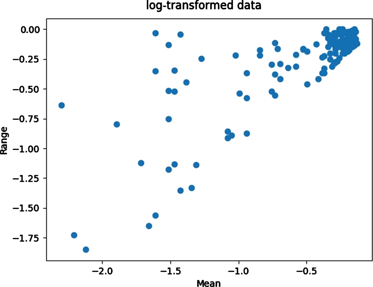
Log transformed data.

It is discovered that the data required 1-month non-seasonal differencing and 12-month seasonal differencing to achieve stationarity using the Augmented Dickey-Fuller Unit Root Test (test statistic=–7.14, and critical values at 0.01=–3.46, 0.05=–2.87, 0.1=–2.57) and evaluating ACF and PACF (Figs. 10, 11) [57]. Eventually, the SARIMA (0, 1, 2) (0, 1, 1)₁₂ model was chosen to be the best fitted for the data used with the lowest AIC = 1526.2759.

Fig. 10

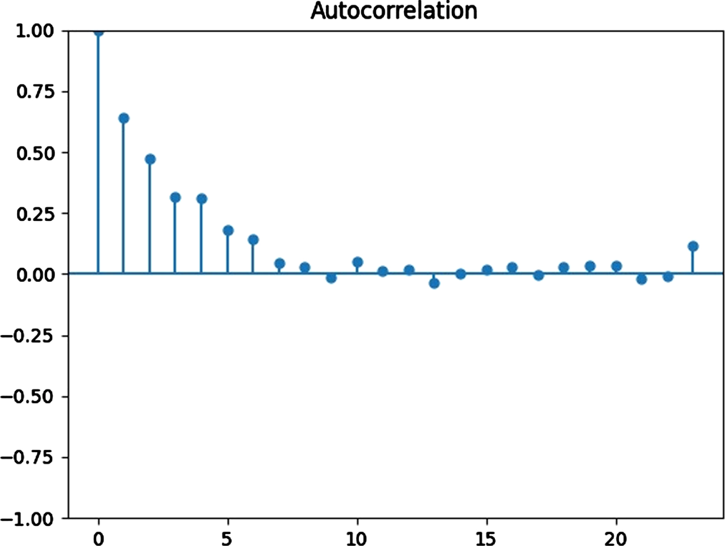
Autocorrelation function plots.

Fig. 11

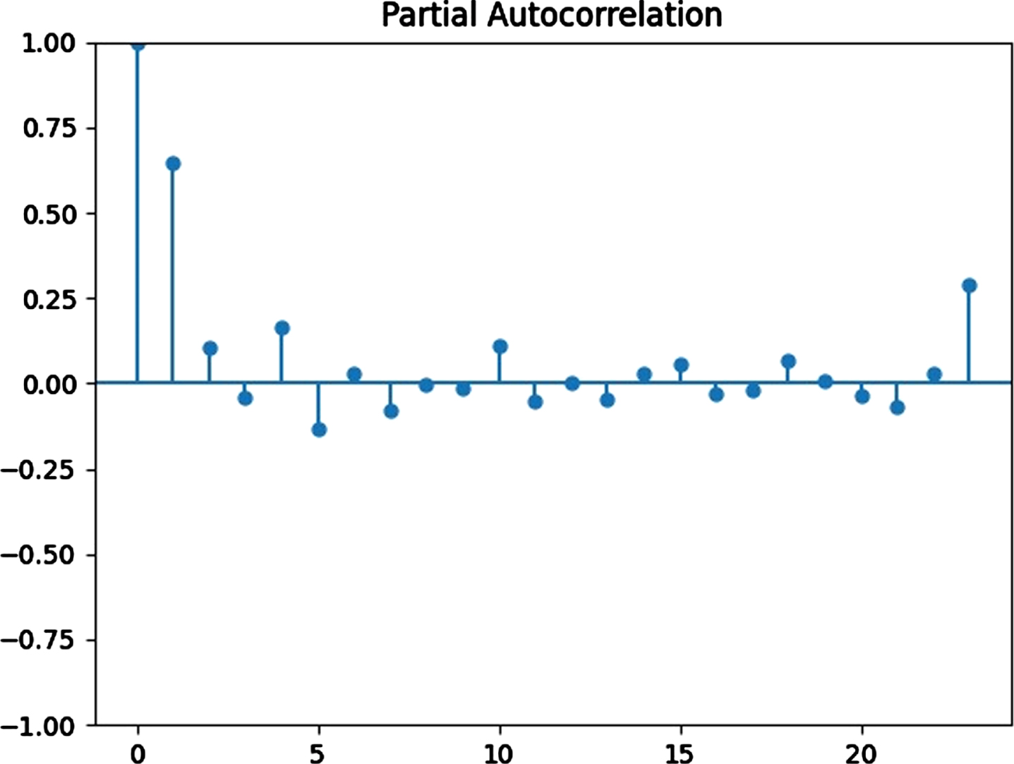
Partial autocorrelation function plots.

Using Pearson’s correlation coefficient, the cross correlation among the independent variables shows that all the variables correlated significantly with each other. The minimum and maximum temperatures were significantly associated with each other, with r = 0.2679. Precipitation and humidity were significantly and negatively correlated with maximum temperature with r = -0.7797 and r = -0.7035 respectively. The results of the cross-correlations also shows that precipitation and humidity correlate positively with r = 0.8159. r = 0.1045, r = 0.0175, r = 0.0666, and r = 0.0182 respectively. Ljung Box Q statistics was 39.67 (p = 0.635), this signifies the regression model is acceptable.

3.1 RSS score

After implementing the forecasting methods described in Sections 2.3, 2.4, and 2.5, time series models SARIMA, ARIMA, and LSTM have RSS values 0.60, 0.91, and 0.72 respectively. This demonstrates that the SARIMA model, as opposed to the ARIMA and LSTM, fits the cholera and climate data the best. In comparison to Modified ARIMA and Modified LSTM, the Modified SARIMA model outperformed all other methods with an RSS = 0.502, making it the model that fits the dataset used the best. The Modified SARIMA makes use of SARIMA because it is more effective at forecasting complicated data with seasonality as a measure because cholera outbreak is a seasonal illness.

3.2 Performance metrics score

The time series model on Cholera namely ARIMA, SARIMA, and LSTM were evaluated by using the performance metrics given in Section 3.1, and the results are presented in Table 1. It is evident that the LSTM model an accuracy = 93% and a MAPE = 0.074, outperforming other models with the best accuracy and the lowest MAPE. When feature extraction using DWT was implemented in all of the methods, the performance of all the models increased. The modified model is termed as Modified LSTM, Modified ARIMA and Modified SARIMA. According to Table 2, MODIFIED SARIMA is more accurate and has a lower error rate than LSTM. With accuracy = 97%, a MAPE = 0.0300, ME = 0.235, MAE = 0.321, and an RMSE = 0.19, the Modified SARIMA model has the least amount of error among all modified models. As a consequence, it was determined that the Modified SARIMA approach is the best way under time series methods for cholera forecasting. Finally, the related parameters are plugged into Equation 7 above and the fitted model SARIMA (0, 1, 2) (0, 1, 1)₁₂ could be written as Equation 20:

$\begin{matrix} (1 - B) (1 - B^{12}) Y_{t} = \\ (1 + θ_{1} B + θ_{2} B^{2}) (1 + θ_{1} B^{12}) w_{t} \end{matrix}$ (20)

Table 1

Comparison of the performance of the models

	Accuracy (%)	MAPE	ME	MAE	RMSE	R-Squared (R²)	Adj R²	RSS
SARIMA Model	91.61	0.084	0.475	1.12	0.054	0.295	0.291	0.60
ARIMA Model	81.76	0.182	0.458	1.18	0.045	0.262	0.258	0.91
LSTM Model	93.0	0.074	0.499	1.00	0.16	0.262	0.258	0.72

Table 2

Comparison of the performance of the modified models

	Accuracy (%)	MAPE	ME	MAE	RMSE	R-Squared (R²)	Adj R²	RSS
Modified SARIMA	97.0	0.0300	0.235	0.321	0.19	0.867	0.864	0.502
Modified ARIMA	96.71	0.0329	0.608	0.671	0.55	0.858	0.855	0.551
Modified LSTM	95.0	0.0482	0.512	0.952	0.23	0.867	0.864	0.600

3.3 Normality test

Quantile-quantile plots (Q-Q plots) and formal normality tests have historically been two popular methods for testing the normality assumption [58]. A common and useful visualization technique for comparing the empirical probability distribution of a random variable to any proposed theoretical distribution is the Q-Q plot. The residuals are approximately normally distributed, according to the Q-Q plot in Fig. 12, since they lie along the 45⁰ line. For the formal normality test, the Shapiro-Wilk test which evaluates the combined hypothesis that the data are independent and identically distributed and normal [59] was used to test for normality. The result shows that the residuals were distributed normally (p = 0.164).

Fig. 12

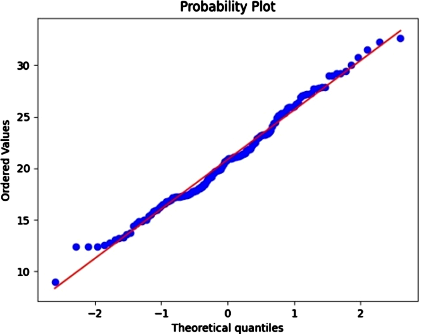
The residual plot of the fitted model and the resulting Q–Q plot.

4 Conclusion

Three time series models, ARIMA, SARIMA, and the LSTM, have employed and assessed. Later, the methods were improved using the DWT in order to have a higher forecasting accuracy and little error. The modified models shown greater promise by offering more precise findings and low error rates. Because it has been improved using DWT, which eliminates duplicated data, and k-means clustering, used to finds and discard outliers that may impair the performance of the model, Modified SARIMA was better than the SARIMA.

The study advises the use of various clustering methods for efficient outlier detection and the addition of socioeconomic data for improved outcome predictions because these factors also affect cholera epidemics and further the disease’s spread.

The result of this research will be important to epidemiologists and health professionals interested in the curtailing of cholera cases by preparing and creating Response Plans. Health professionals can prepare potential coping and adaptation strategies for potential health risks associated with climate change in Nigeria which will aid in fulfilling the Global Taskforce on Cholera Control (GTFCC) 2030 mandate on cholera “Roadmap to End Cholera by 2030”.

Footnotes

Funding and conflicts of interests

This research is not funded by any agency. The authors declare no conflict of inter.

References

Mengel

M.A.

, Delrieu

, Heyerdahl

and Gessner

B.D.

, Cholera Outbreaks in Africa, (2014), 117–144, doi: 10.1007/82.

Asunduwa

et al., Descriptive analysis of a cholera outbreak in 14 LGAs of Sokoto State – Nigeria, Int. J. Infect. Dis. 101 (2020), 363, doi: 10.1016/j.ijid.2020.09.951.

Deen

, Mengel

M.A.

and Clemens

J.D.

, Epidemiology of cholera, Vaccine, vol. 38. Elsevier Ltd, pp. A31–A40, Feb. 29 2020, doi: 10.1016/j.vaccine.2019.07.078.

Elimian

et al., Epidemiology, diagnostics and factors associated with mortality during a cholera epidemic in Nigeria, October 2020-October 2021: a retrospective analysis of national surveillance data, BMJ Open 12(9) (2022), 1–16, doi: 10.1136/bmjopen-2022-063703.

Dan-Nwafor

C.C.

et al., A cholera outbreak in a rural north central Nigerian community: An unmatched case-control study, BMC Public Health 19(1) (2019), 1–7, doi: 10.1186/s12889-018-6299-3.

Bwire

et al., Epidemiology of cholera outbreaks and socio-economic characteristics of the communities in the fishing villages of Uganda: 2011-2015, PLoS Negl. Trop. Dis. 11(3) (2017), 2011–2015, doi: 10.1371/journal.pntd.0005407.

Teri

, Musa and O. Samuel Olayemi, APPLICATION OF LOGISTIC REGRESSION MODELS FOR THE EVALUATION OF CHOLERA OUTBREAK IN ADAMAWA STATE NIGERIA, Int. J. Math. Stat. Stud. 8(1) (2020), 32–54.

Dalhat

M.M.

et al., Descriptive characterization of the cholera outbreak in Nigeria, BMC Public Health 14(1) (2014), 1–7, doi: 10.1186/1471-2458-14-1167.

Bompangue

et al., Cholera epidemics, war and disasters around Goma and Lake Kivu: an eight-year survey, PLoS Negl. Trop. Dis. 3(5) (2009), doi: 10.1371/journal.pntd.0000436.

10.

Marin

M.A.

et al., Cholera Outbreaks in Nigeria Are Associated with Multidrug Resistant Atypical El Tor and Non-O1 / Non- O139 Vibrio cholerae, 7(2) (2013), doi: 10.1371/journal.pntd.0002049.

11.

Min

X.U.

, Chunxiang

C.A.O.

, Duochun

, Biao

K.A.N.

, Huicong

J.I.A.

and Yunfei

X.U.

, District prediction of cholera risk in China based on environmental factors, 58(23) (2013), 2798–2804, doi: 10.1007/s11434-013-5776-4.

12.

Perez-Saez

et al., The seasonality of cholera in sub-Saharan Africa: a statistical modelling study, Lancet Glob. Heal. 10(6) (2022), e831–e839, doi: 10.1016/S2214-109X(22)00007-9.

13.

Zheng

et al., Cholera outbreaks in sub-Saharan Africa during 2010-2019: a descriptive analysis, Int. J. Infect. Dis. 122 (2022), 215–221, doi: 10.1016/j.ijid.2022.05.039.

14.

Wilson

A.M.

, The spread of cholera to and within Nigeria 1970-71, J Clin Pathol. 24(8)(768) (1970), 1970, doi: Doi:10.1136/jcp.24.8.768-c.

15.

Lessler

et al., Mapping the burden of cholera in sub-Saharan Africa and implications for control: an analysis of data across geographical scales, Lancet 391(10133) (2018), 1908–1915, doi: 10.1016/S0140-6736(17)33050-7.

16.

Babatimehin

O.I.

, Uyeh

J.O.

and Onukogu

A.U.

, Analysis of the Re-emergence and Occurrence of Cholera in Lagos State, Nigeria, Bull. Geogr. 36(36) (2017), 21–32, doi: 10.1515/bog-2017-0012.

17.

Salubi

E.A.

and Elliott

S.J.

, Geospatial analysis of cholera patterns in Nigeria: findings from a cross-sectional study, BMC Infect. Dis. 21(1) (2021), doi: 10.1186/s12879-021-05894-2.

18.

Rebaudet

, Sudre

, Faucher

and Piarroux

, Environmental determinants of cholera outbreaks in inland africa: A systematic review of main transmission foci and propagation routes, J. Infect. Dis. 208(SUPPL. 1) (2013), doi: 10.1093/infdis/jit195.

19.

Usmani

, Brumfield

K.D.

, Jamal

, Huq

, Colwell

R.R.

and Jutla

, A review of the environmental trigger and transmission components for prediction of cholera, Trop. Med. Infect. Dis. 6(3) (2021), doi: 10.3390/tropicalmed6030147.

20.

Agarwal

and Verma

, Modeling and Analysis of the Spread of an Infectious Disease Cholera with Environmental Fluctuations, 7(1) (2012), 406–425.

21.

Stoltzfus

J.D.

et al., Interaction between climatic, environmental, and demographic factors on cholera outbreaks in Kenya, Infect. Dis. Poverty 3(1) (2014), 1–9, doi: 10.1186/2049-9957-3-37.

22.

Leckebusch

G.C.

and Abdussalam

A.F.

, Climate and socioeconomic influences on interannual variability of cholera in Nigeria, 107–117, Heal. Place 34 (2015), doi: 10.1016/j.healthplace.2015.04.006.

23.

Daisy

S.S.

, Islam

A.K.M. Saiful

, Akanda

A.S.

, Faruque

A.S.G.

, Amin

and Jensen

P.K.M.

, Developing a forecasting model for cholera incidence in Dhaka megacity through time series climate data, J. Water Health 18(2) (2020), 207–223, doi: 10.2166/wh.2020.133.

24.

de Magny

G. Constantin

, Cazelles

and Guégan

J.-F.

, Cholera Threat to Humans in Ghana Is Influenced by Both Global and Regional Climatic Variability, Ecohealth 3(4) (2006), 223–231, doi: 10.1007/s10393-006-0061-5.

25.

Fernández

M.Á. Luque

, Bauernfeind

, Jiménez

J.D.

, Gil

C.L.

, Omeiri

N. El

and Guibert

D.H.

, Influence of temperature and rainfall on the evolution of cholera epidemics in Lusaka, Zambia, 2003–2006: analysis of a time series, Trans. R. Soc. Trop. Med. Hyg. 103(2) (2009), 137–143, doi: 10.1016/j.trstmh.2008.07.017.

26.

Reyburn

, Kim

D.R.

, Emch

, Khatib

, Von Seidlein

and Ali

, Climate variability and the outbreaks of cholera in Zanzibar, East Africa: A time series analysis, Am. J. Trop. Med. Hyg. 84(6) (2011), 862–869, doi: 10.4269/ajtmh.2011.10-0277.

27.

Paz

, Impact of Temperature Variability on Cholera Incidence in Southeastern Africa, 1971–2006, Ecohealth 6(3) (2009), 340–345 doi: 10.1007/s10393-009-0264-7.

28.

Wierzba

T.F.

, Oral cholera vaccines and their impact on the global burden of disease, 15(6) (2019), 1294–1301.

29.

Shaikh

, Lynch

, Kim

and Excler

J.L.

, Current and future cholera vaccines, Vaccine 38 (2020), A118–A126, doi: 10.1016/j.vaccine.2019.12.011.

30.

Kotsiantis

, Kanellopoulos

and Pintelas

P.E.

, Handling imbalanced datasets: A review Handling imbalanced datasets: A review, no. May 2014, 2005.

31.

Alfred

and Obit

J.H.

, The roles of machine learning methods in limiting the spread of deadly diseases: A systematic review, Heliyon 7 no. 6. Elsevier Ltd, Jun. 01, 2021, doi: 10.1016/j.heliyon.2021.e07371.

32.

Nguyen

C.H.

, Thi

and Anh

, Using Local Weather and Geographical Information to Predict Cholera Outbreaks in Hanoi, Vietnam Using Local Weather and Geographical Information to Predict Cholera Outbreaks in Hanoi, Vietnam, no. October 2017, 2016, doi: 10.1007/978-3-319-38884-7.

33.

Chau

N.H.

, Enhancing Cholera Outbreaks Prediction Performance in Hanoi, Vietnam Using Solar Terms and Resampling Data, LNAI 10448 (2017), 266–276, doi: 10.1007/978-3-319-67074-4_26.

34.

Badkundri

, Valbuena

, Pinnamareddy

, Cantrell

and Standeven

, Forecasting the 2017-2018 Yemen Cholera Outbreak with Machine Learning, pp. 1–27, Feb. 2019, [Online]. Available: http://arxiv.org/abs/1902.06739.

35.

Leo

, Luhanga

and Michael

, Machine Learning Model for Imbalanced Cholera Dataset in Tanzania, Sci. World J. 2019 (2019), doi: 10.1155/2019/9397578.

36.

Campbell

A.M.

, Racault

M.F.

, Goult

and Laurenson

, Cholera risk: A machine learning approach applied to essential climate variables, Int. J. Environ. Res. Public Health 17(24) (2020), 1–24, doi: 10.3390/ijerph17249378.

37.

Ali

, Kim

D.R.

, Yunus

and Emch

, Time Series Analysis of Cholera in Matlab, Bangladesh, during 1988-2001, 31(1) (2013), 11–19.

38.

Gursoy

M.İ.

, Ustun

S.V.

and Yilmaz

A.S.

, An Efficient DWT and EWT Feature Extraction Methods for Classification of Real Data PQ Disturbances, 2018.

39.

Kotsiantis

S.B.

and Kanellopoulos

, Data preprocessing for supervised leaning, Int. J. Comput. Sci. 1(2) (2006), 1–7, doi: 10.1080/02331931003692557.

40.

Alegeh

, Thottoli

, Mian

and Longstaff

, Feature Extraction of Time-Series Data Using DWT and FFT for Ballscrew Condition Monitoring, (2021), 402–407 10.3233/ATDE210069.

41.

Rinky

B.P.

, Mondal

, Manikantan

and Ramachandran

, DWT based feature extraction using edge tracked scale normalization for enhanced face recognition, 6 (2012), 344–353, doi: 10.1016/j.protcy.2012.10.041.

42.

Chaovalit

, Gangopadhyay

, Karabatis

and Chen

, Discrete Wavelet Transform-Based Time Series Analysis and Minin, 43(2) (2011), doi: 10.1145/1883612.1883613.

43.

Batal

and Hauskrecht

, A Supervised Time Series Feature Extraction Technique using DCT and DWT, (2009), doi: 10.1109/ICMLA.2009.13.

44.

Santhanam

and Padmavathi

M.S.

, Application of K-Means and genetic algorithms for dimension reduction by integrating SVM for diabetes diagnosis, Procedia Comput. Sci. 47(C) (2015), 76–83, doi: 10.1016/j.procs.2015.03.185.

45.

Afrin

and Tabassum

, Comparative Performance Of Using PCA With K-Means And Fuzzy C Means Clustering For Customer Segmentation, Comp. Perform. Using PCA With K-Means Fuzzy C Means Clust. Cust. Segmentation 4(10) (2015), 70–74.

46.

Box

, Box and Jenkins: Time Series Analysis, Forecasting and Control BT - A Very British Affair: Six Britons and the Development of Time Series Analysis During the 20th Century, T.C. Mills, Ed. London: Palgrave Macmillan UK (2013), 161–215 .

47.

Elmasdotter

, LSTM and ARIMA for sales A comparative study between LSTM and ARIMA for sales forecasting in retail, 2018.

48.

Shih

and Rajendran

, Comparison of Time Series Methods and Machine Learning Algorithms for Forecasting Taiwan Blood Services Foundation’s Blood Supply, J. Healthc. Eng. 2019 (2019), doi: 10.1155/2019/6123745.

49.

Arunkumar

K.E.

, Kalaga

D.V.

, Mohan

, Kumar

and Brenza

T.M.

, Comparative analysis of Gated Recurrent Units (GRU), long Short-Term memory (LSTM) cells, autoregressive Integrated moving average (ARIMA), seasonal autoregressive Integrated moving average (SARIMA) for forecasting COVID-19 trends, Alexandria Eng. J. 61(10) (2022), 7585–7603, doi: 10.1016/j.aej.2022.01.011.

50.

Liu

et al., Forecast of the trend in incidence of acute hemorrhagic conjunctivitis in China from – using the Seasonal Autoregressive Integrated Moving Average (SARIMA) and Exponential Smoothing (ETS) models, J. Infect. Public Health 13(2) (2020), 287–294, doi: 10.1016/j.jiph.2019.12.008.

51.

Bowerman

B.L.

, O’Connell

R.T.

Forecasting and time series: an applied approach, 3rd ed. Belmont, Calif. SE -: Duxbury Press, 1993.

52.

Hochreiter

and Schmidhuber

, Long Short-term Memory, Neural Comput. 9 (1997), 1735–1780, doi: 10.1162/neco.1997.9.8.1735.

53.

Lee

et al., Long short-term memory recurrent neural network-based acoustic model using connectionist temporal classification on a large-scale training corpus, China Commun. 14(9) (2017), 23–31, doi: 10.1109/CC.2017.8068761.

54.

Mamudu

, Yahaya

and Dan

, Application of Seasonal Autoregressive Integrated Moving Average (SARIMA) For Flows of River Kaduna, 28(2) (2021).

55.

and Chang

E.Y.

, KBA: kernel boundary alignment considering imbalanced data distribution, IEEE Trans. Knowl. Data Eng. 17(6) (2005), 786–795, doi: 10.1109/TKDE.2005.95.

56.

and

and Cheng

H.T.U.

, On residual sums of squares in non-parametric autoregression, Stoch. Process. their Appl. 48 (1993), 157–174.

57.

Dickey

D.A.

and Fuller

W.A.

, Distribution of the Estimators for Autoregressive Time Series with a Unit Root, J. Am. Stat. Assoc. 74(366a) (1979), 427–431, doi: 10.1080/01621459.1979.10482531.

58.

Huang

K.-W.

, Qiao

, Liu

, Dai

, Liu

, Computer Vision and Metrics Learning for Hypothesis Testing: An Application of Q-Q Plot for Normality Test, 2019.

59.

Shapiro

S.S.

and Wilk

M.B.

, An analysis of variance test for normality (complete samples)†, Biometrika 52(3–4) (1965), 591–611, doi: 10.1093/biomet/52.3-4.591.