Aero-engine residual life prediction based on time-series residual neural networks

Abstract

In order to address the timing problem, invalid data problem and deep feature extraction problem in the current deep learning based aero-engine remaining life prediction, a remaining life prediction method based on time-series residual neural networks is proposed. This method uses a combination of temporal feature extraction layer and deep feature extraction layer to build the network model. First, the temporal feature extraction layer with multi-head structure is used to extract rich temporal features; then, the spatial attention mechanism is applied to improve the weights of important data; finally, the deep feature extraction layer is used to process the deep features of the data. To verify the effectiveness of the proposed method, experiments are conducted on the C-MAPSS dataset provided by NASA. The experimental results show that the method proposed in this paper can make accurate predictions of the remaining service life under different sub-datasets and has outstanding performance advantages in comparison with other outstanding networks.

Keywords

Time sequential resnet temporal feature extraction layer spatial attention module deep feature extraction layer remaining useful life Introduction

1 Introduction

With the rapid development of modern industry, there is an increasing demand for the safety of large instruments, prognostic and health management (PHM) [1, 2] is gaining unprecedented interest and generating huge market demand in areas such as aerospace, automotive manufacturing, wind power and many others. PHM includes fault diagnosis [3], abnormal state detection, and remaining useful life prediction (RUL) [4], and so on. It has a great prospect in engineering applications.

The current mainstream approach to life prediction is to use neural networks to extract features from the data and predict the remaining life of the target by building a predictive model. Zhao et al [5]. proposed the fitting curve derivative method of maximum power spectrum density to extract target performance degradation characteristics from historical data, then the life prediction model is constructed to realize the remaining life prediction. Cheng et al [6]. adopted transferable convolutional neural network to learn regional invariant features, and used convolutional neural network to extract degradation features, so as to predict the remaining life. Qin et al [7]. proposed taking the root mean square at different times as a health indicator, and then using the double-gated attention unit to predict the future health indicator sequence. Ma et al [8]. extracted several classical time and frequency domain features, respectively, and used the isometric mapping method to extract the backbone components of these features, the fused feature information is filtered through a microscopic attention mechanism and then fed into a long and short term memory network for prediction. Li et al. [9] used particle filter to fuse multi-sensor signals to estimate the system state, and used the priority sensor group selection algorithm to select the information sensors. The algorithm first prioritized the sensors according to their single performance in RUL prediction, and then selected the optimal sensor group according to their comprehensive performance. Wen et al. [10] proposed a nonlinear data fusion method based on genetic programming to construct a better composite HI. In this way, multiple condition monitoring signals are fused together to provide better predictive capabilities. Li et al. [11] proposed an intelligent remaining useful life prediction method based on deep learning, which uses time-frequency domain information for prediction, and uses convolutional neural network to realize multi-scale feature extraction. Liu et al. [12] decomposed the original battery capacity data into some intrinsic mode functions and a residual after adopting the empirical mode decomposition method. Then, the LSTM submodel is used to estimate the residual and the Gaussian process regression submodel is used to fit the uncertainty. Wang et al. [13] studied the bearing fault diagnosis method based on wavelet transform, analyzed the bearing early defect features, and used the health index algorithm to fuse the extracted features to characterize the bearing defect state. The empirical physics knowledge and statistical model under the Bayesian framework are used to predict the remaining useful life of bearings with uncertainty quantification by recursive particle filtering. Ren et al. [14] proposed a multidimensional feature extraction method based on an autoencoder model to characterize battery health degradation. Ren et al. [15] proposed a feature vector based on time-frequency wavelet joint features to effectively characterize the bearing degradation process. Wang [16] used relevance vector machine regression with different kernel parameters to sparsely represent the degradation data of bearings.

From the above analysis, it can be seen that the research of data-driven residual life prediction mainly focuses on the extraction method of performance degradation features, and ignores the time series problems, complex and useless data problems and difficult to extract deep features caused by too large data sets, such as aero-engine data sets. Time series problems increase with the amount of input data, and the inability to correlate current moment data features with historical features leads to unsatisfactory network results. The problem of useless data refers to that when processing large data sets, not all the data is related to RUL research, and the useless data will increase the complexity of the network. In a network with certain computational power, the useless data will often make the neural network unable to extract features correctly. The difficulty in extracting deep features mainly occurs in large data sets. Due to the large amount of data, generally shallow network cannot effectively extract features, and deep network will bring gradient explosion problem. To solve these problems, this paper proposes a new forecasting method of aero-engine residual life based on Time Sequental residual network (TSresnet). The innovations of this paper are as follows: (1) We propose to use a temporal feature extraction layer with multi-head structure for data extraction, which avoids the temporal problem limited by the size and shape of the convolution kernel. (2) The attention mechanism is used to improve the weights of effective data and reduce the impact of invalid data on the network. (3) The residual connection between the network layers is used to avoid the problem of deep feature extraction and gradient explosion caused by the limitation of the number of network layers when extracting deep features.

2 Residual life prediction model based on time-series residual networks

2.1 Time-series feature extraction layer

The TSresnet proposed in this paper is inspired by the convolutional neural network and dilated causal convolution. Aiming at the problem that the existing methods have defects in the receptive field and fail to demonstrate their capabilities and characteristics in other fields, it is improved, so that its scope of use is not limited to the field of image processing, and it also has excellent results in the field of fault prediction and diagnosis and remaining life prediction.

Convolutional neural networks [17 –19] are very important network structures in deep learning and are widely used in many industries such as image processing, fault prediction and diagnosis, CNN obtains the feature map of the next layer through the convolution operation of the convolution layer. The key calculation formulas are given in Equations (1), (2), and (3). $W_{out} = \frac{(W_{in} + 2 P - w)}{s} + 1$ (1) $H_{out} = \frac{(H_{in} + 2 P - h)}{s} + 1$ (2) $D_{out} = k$ (3)

W_in and H_in are the width and height of the input feature map, W_out and H_out are the width and height of the output feature map, s is the moving step, P is the padding parameter, and k is the number of convolution kernels.

Using images as input, CNN can effectively extract a large number of features from the input feature map, avoiding complex feature extraction work. But as their applications become more widespread, their limitations arise.Because its receptive field is relatively fixed, time-series problems arise when working with large data sets, where current features are not well correlated with historical features. In order to solve the temporal problem of large data sets, dilated causal convolution(DCC) [20, 21] has been proposed.

The flexible receptive field of DCC can capture rich temporal features. The number of layers, the size of convolution kernel, and the expansion coefficient of DCC can be freely selected according to different environments. Compared with other structures, its memory consumption is lower, which makes it have high performance-price ratio and generalization ability. The DCC receptive field is shown in Fig. 1.

Fig. 1

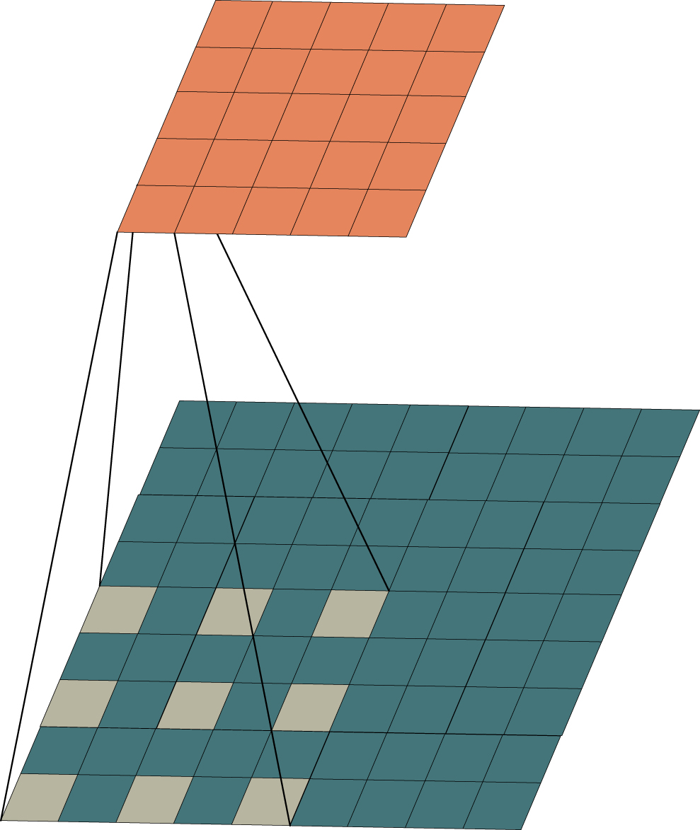
The DCC receptive field.

The existence of the expansion coefficient can effectively increase the receptive field of DCC, making DCC more flexible than CNN. At the same time, the design of the convolution kernel size can make DCC focus on specific areas for feature extraction, which is one of the advantages of DCC. The key calculation formulas are given in Equations (4), (5), and (6). $k^{'} = k + (k - 1) \times (d - 1)$ (4) ${RF}_{i + 1} = {RF}_{i} + (k_{i}^{'} - 1) \times S_{i}$ (5) $S_{i} = \prod_{j = 1}^{i} {Stride}_{j} = S_{i - 1} \times {Stride}_{i}$ (6)

Where k′ is the equivalent convolution kernel size; k is the size of convolution kernel; d is the expansion coefficient; RF_i is the receptive field of layer i; RF_i+1 is the receptive field of layer i + 1; S_i is the product of all steps up to layer i; Stride_j is the step size of the j layer. Its RF_i+1 is affected by three aspects: S_i, k′, and d. The larger the three parameters of S_i, k′, and d, the larger the DCC receptive field will be.

The expansion of DCC receptive field brings richer time-series features, but at the same time, holes are inserted in the convolution kernel, and the holes also have feature information, which leads to the loss of some features when DCC extracts features. In response to the above problems, this paper proposes a timing feature extraction layer with a multi-head structure, which has both the flexible feeling field of DCC and avoids the loss of information in the empty part, and has been verified through several experiments that this structure has significant advantages in the ability of extracting data time-series information, and is more capable of extracting time-series features than the single-head structure. Its specific structure is shown in Fig. 2.

Fig. 2

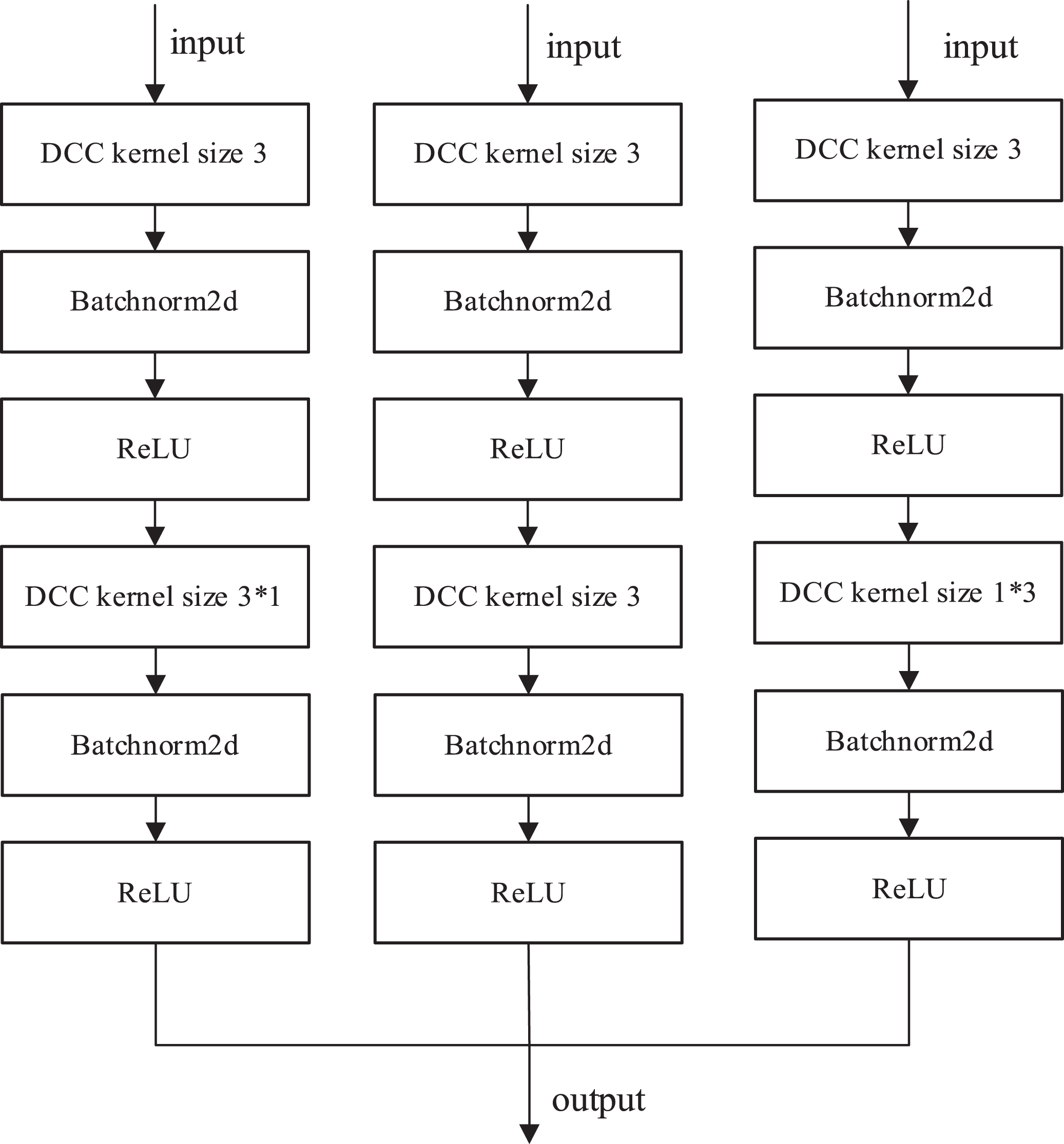
Time-series feature extraction layer.

The first DCC of the three heads in the time series feature extraction layer uses the DCC with the convolution kernel size of 3×3, stride of 3, and dilation factor of 1, the dimensionality of the data is reduced into a feature matrix. Then Batchnorm2d is used to normalize the data, which can limit the data to a range of mean 0 and variance 1, so that the data distribution is consistent to avoid the disappearance of the gradient. The calculation formula is given in Equation (7). $y = \frac{x - E [x]}{\sqrt{V_{ar} [x] + ɛ}} * γ + β$ (7)

Where x is the input; y is the output, E [x] is the input mean; V_ar [x] is the input variance; ɛ is 1e^-5 and its function is mainly to prevent the denominator from being zero; γ is 1; β is 0.

ReLU is the activation function, which is essentially a piecewise linear function. Using ReLU can make the network simpler and faster in calculation, and the use of Batchnorm2d and ReLU can greatly simplify the complexity of calculation. The parameters of the second layer DCC from left to right are the DCC with convolution kernel size 3×1, stride 1, and dilation factor 2, the DCC with convolution kernel size 3×3, stride 1, and dilation factor 1, and the DCC with convolution kernel size 1×3, stride 1, and dilation factor 2. The design of three different convolution kernels can fill the features of the hole part in DCC and expand its receptive field to capture rich time-series features. 3×1 is mainly used for feature extraction of column data, and combined with the actual data set, it is to extract the features of a single sensor over time. 1×3 is mainly used for feature extraction of row data, and combined with the actual data set, it is to extract features of different sensors at the same time. 3×3 aims at the feature extraction of global changes, and the superposition of the three feature structures can obtain a matrix with rich time-series features. Its receptive field display on the dataset is shown in Fig. 3.

Fig. 3

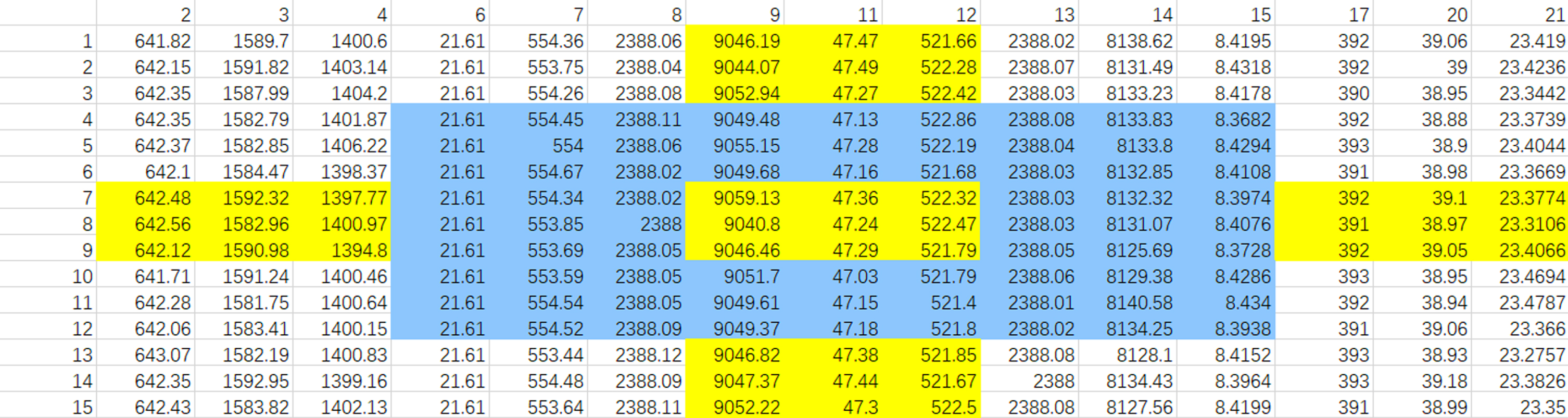
Schematic representation of the receptive field of the dataset.

In the figure, the first column is the time serial number, and the first row is the sensor number. When extracting features from the central yellow area, the three-head structure of the time-series feature extraction layer can extract features from a larger area. Compared with the feature range extracted by a single head, the three-head structure covers all the row features and column features in the blue part of the figure.

The network structure parameters in this paper are the optimal results obtained through multiple experiments. The first layer DCC selection experiment is shown in Fig. 4.

Fig. 4

DCC kernel size parameter selection experiment.

The experiment used different kernel_size for loss function experiments, set the number of iterations to 200, and compared the size of the loss function, the experimental results show that the loss function of the first layer DCC decreases to the lowest when kernel_size is 3, which indicates that the loss function decreases the fastest when kernel_size is 3, and the performance is more stable, so kernel_size is determined to be 3.

2.2 Deep feature extraction layer

In order to solve the problem that it is difficult to extract deep features caused by large datasets, two aspects are dealt with in this paper. (1) In the data preprocessing stage, the data that does not change in the whole life of the system will be removed, leaving the relatively pure data that changes with the degradation of the system. (2) An attention mechanism (AM) [22] is added to the deep feature extraction layer.

AM has made significant contributions to image fault detection and other fields, and has been proved to be beneficial to improve the performance of neural networks. AM is a mechanism to focus local key information. In principle, AM is classified into three types: Spatial Attention Module (SAM), Channel Attention Module (CAM) and Spatial Channel Hybrid (SCAM). SAM is to find the data that is most sensitive to the change of results in the data and increase its weight. SAM is selected to join the network in this experiment, and SAM can improve the weight of a single data to realize the enhanced extraction of important features. The structure of SAM is shown in Fig. 5.

Fig. 5

Spatial attention mechanism.

The incoming data is first dimensioned down to a two-channel feature by using a max pooling layer and an average pooling layer, and then the two-channel feature is convolved using a convolution layer to form a single-channel feature, which is then passed into a Sigmoid function. The role of the Sigmoid function is to map the real input to the interval (0,1), so that it becomes a weight for the individual feature values. The Sigmoid function is expressed in Equation (8): $σ (z) = \frac{1}{1 + e^{- z}}$ (8)

The data features are reset by SAM and then connected to the Dropout layer and residual block, which together form the deep feature extraction layer structure. The Dropout layer can randomly set the hidden layer neurons to zero according to the coefficients, and the zero neurons are not fixed in each batch, so that the network parameter update does not have to propagate completely according to a certain path. The benefit of this design is to prevent the network from overfitting, increase the robustness of the network, and make the network output more accurate. This is shown in Fig. 6.

Fig. 6

Dropout.

Part of the features of the residual block [23] will be divided into two branches, one branch enters the convolutional layer to operate with the activation function, and the other branch directly adds the matrix with the participating branches without processing, and then activates after addition, which requires that the output size of the two branches must be consistent. This structure can effectively avoid the problem of gradient disappearance caused by the improvement of network depth. By wrapping the input information around the output of the network, it not only extracts the characteristics of the input but also protects the integrity of the input information. The residual block structure is shown in Fig. 7.

Fig. 7

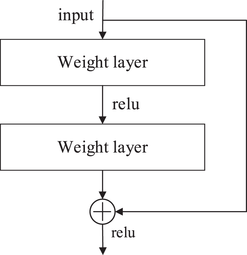
Residual blocks.

The parameters of the deep feature extraction layer composed of SAM, Dropout and residual block are shown in Table 1.

Table 1

Deep feature extraction layer structure

Network layer name	Parameter
SAM	*
Dropout	0.2
ConvBlock 1	5×5, 64, strider 1 3×3, max pool, strider 2
ConvBlock 2	$[\begin{matrix} 3 \times 3 & 64 \\ 3 \times 3 & 64 \end{matrix}] \times 2$
ConvBlock 3	$[\begin{matrix} 3 \times 3 & 128 \\ 3 \times 3 & 128 \end{matrix}] \times 2$
ConvBlock 4	$[\begin{matrix} 3 \times 3 & 256 \\ 3 \times 3 & 256 \end{matrix}] \times 2$
ConvBlock 5	$[\begin{matrix} 3 \times 3 & 512 \\ 3 \times 3 & 512 \end{matrix}] \times 2$
Dropout	0.2
Classification	Average pool 131Fc

In order to prevent the network from overfitting, a Dropout layer is added to the network, and the Dropout layer coefficient is set to 0.2. ConvBlock1, ConvBlock2, ConvBlock3, ConvBlock4 and ConvBlock5 are residual blocks of different convolution sizes and number of channels, which are connected by way of residual linkage to flatten the feature information for more effective extraction of deeper features of the data, and then connected to Classification to output prediction results.

2.3 Time-series residual neural networks (TSresnet)

TSresnet is divided into two parts at the design level, one is composed of time-series feature extraction layer, and the other is composed of a deep feature extraction layer. The time-series feature extraction layer firstly extracts the data time-series information, and then transmits the temporal information to the deep feature extraction layer to extract its deep features, completing the TSresnet’s extraction of deep temporal features. The TSresnet structure is shown in Fig. 8.

Fig. 8

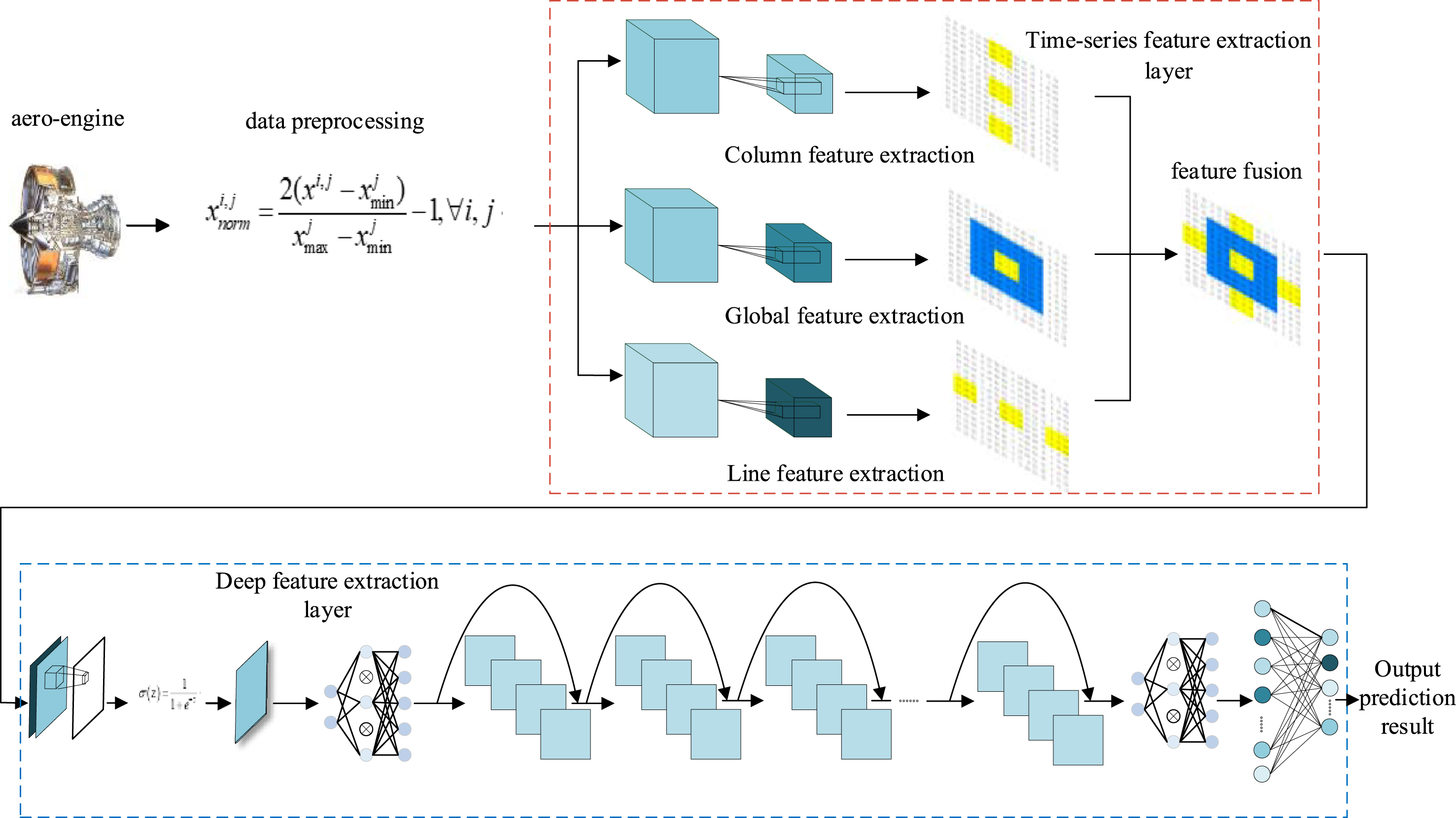
Network structure diagram of TSresnet.

3 Experimental study

3.1 The C-MAPSS dataset

To test the performance of TSresnet, this paper uses the C-MAPSS dataset [24] published by NASA, a dataset released by NASA for a PHM-themed competition. NASA, as the global head agency in aerospace, has made many significant contributions to the world, and there is a strong credibility to use NASA data for lifetime prediction. The dataset uses C-MAPSS to simulate the supersonic Turbofan engine. The dataset consists of four sub-datasets, which are composed of data collected by 21 sensors and contain all historical data from operation to failure. The data set contains 26 columns of data, the first column is the engine number, the second column is the time period number, and the third to fifth columns are the operation Settings, columns 6 to 26 show the values of 21 sensors (such as velocity, pressure, temperature, etc.). For more information about 21 sensors, see [25]. The engine operates normally at the beginning of each time series and fails at some point in the series. In the training set, the degree of failure increases until the system fails, while in the test set, the time period sequence and sensor data end at some time before the failure. To verify the accuracy of the test set, the data set also provides values for the true remaining useful life (RUL) for the test data. The C-MAPSS dataset details are shown in Table 2, and the sub-datasets are FD001, KD002, FD003 and FD004, respectively.

Table 2
C-MAPSS dataset

C-MAPSS

FD001 FD002 FD003 FD004

Number of training sets 100 260 100 249

Number of test sets 100 259 100 248

Working condition 1 6 1 6

Failure mode 1 1 2 2

Train sample 17731 48819 21820 57522

Test sample 100 259 100 248

C-MAPSS
Number of training sets	100	260	100	249
Number of test sets	100	259	100	248
Working condition	1	6	1	6
Failure mode	1	1	2	2
Train sample	17731	48819	21820	57522
Test sample	100	259	100	248

3.2 Data analysis and preprocessing

The C-MAPSS dataset contains the test data of 21 sensors, and its volume size has exceeded the normal dataset by several times. Traditional networks cannot effectively deal with large data sets, so the process of processing C-MAPSS dataset will produce the time-series problems, invalid data problems and effective deep feature extraction problems targeted by TSresnet. The measured data from some sensors in the C-MAPSS dataset have a constant output over the full life cycle of the engine and they do not provide valid information for the RUL, therefore, six of the sensor data were excluded and the data from 15 sensors were selected as the original input features with the designations 2, 3, 4, 6, 7, 8, 9, 11, 12, 13, 14, 15, 17, 20, 21.

For the four sub-datasets in C-MAPSS, the original data of 15 sensors are normalized to the range of [–1,1]. The formula is given in Equation (9): $x_{norm}^{i, j} = \frac{2 (x^{i, j} - x_{min}^{j})}{x_{max}^{j} - x_{min}^{j}} - 1, \forall i, j$ (9)

Where x^i,j is the i original data of the j sensor, $x_{norm}^{i, j}$ is the normalized value of x^i,j, $x_{max}^{j}$ and $x_{min}^{j}$ are the maximum and minimum values in the original data measured by the j sensor, respectively.

The network parameters are selected as shown in the following table.

3.3 Performance evaluation standard

To test the performance of the TSresnet network, we use three metrics to rate our proposed approach, SCORE, RMSE, and R-squared.

For the degradation process of the engine, early prediction is better than late prediction, so in SCORE, the function before and after the true failure time is asymmetric, and later predicted values are penalized more than earlier ones. The formula is given in Equation (10): $s = {\begin{matrix} \sum_{i = 1}^{n} e^{- (\frac{d_{i}}{a_{1}})} - 1 \dots \dots d_{i} < 0 \\ \sum_{i = 1}^{n} e^{(\frac{d_{i}}{a_{2}})} - 1 \dots \dots d_{i} ⩾ 0 \end{matrix}$ (10)

Where s is the final score; n is the number of test samples; a₁, a₂ are constants 10,13 respectively; d_i is the error between the predicted value and the true value of the i sample. The difference between the early prediction and the late prediction is achieved by contrasting the size of d_i using a different formula.

RMSE is an index describing the dispersion degree between the predicted value and the real value. The smaller the RMSE value is, the smaller the dispersion degree between the predicted value and the real value is, and the more stable the network output result is. The RMSE formula is shown in Equation (11): $RMSE = \sqrt{\frac{1}{N} \sum_{i = 1}^{n} d_{i}^{2}}$ (11)

Where n is the number of test samples; d_i is the error between the predicted value and the true value of the i sample.

R-squared is an evaluation metric to measure the degree of network fit, essentially using the baseline residuals and a measure of the existing network residuals and, in general, using the mean value as the baseline, under normal circumstances R-squared takes values in the range of [0,1], the closer to 1 represents the higher the degree of network fit, R-squared formula as in Equation (12). $R^{2} = 1 - \frac{\sum_{i = 1}^{n} ({\hat{y}}_{i} - y_{i})^{2}}{\sum_{i = 1}^{n} (\bar{y} - y_{i})^{2}}$ (12)

Where ${\hat{y}}_{i}$ is the i predicted value; y_i is the i true value and $\bar{y}$ is the mean.

3.4 Verification of method effect

To demonstrate the superiority of this network over other networks, this paper uses (1) CNN-GRU [26], a neural network with excellent predictive performance; (2) DCN [27], which excels on the bearing dataset with the same rotating body; (3) SE-ResNet50 [28], which is widely recognized by the academic community; as comparison objects, on the basis of the above three kinds of networks, the following four groups of experiments were done: Experiment 1 Loss function comparison experiment, loss function is used to express the gap between the predicted value and the true value, which can effectively show the robustness of the network; experiment 2 Performance evaluation experiment, SCORE, RMSE, R-squared were used as the index of network performance evaluation; experiment 3 Single aero-engine life prediction experiment, showing the change of single engine prediction value; experiment 4 Ablation experiment, (1) remove the time-series feature extraction layer, (2) remove the deep feature extraction layer, ablation experiments are crucial for deep learning research and are the most direct way to study causality innetworks.

3.4.1 Loss function comparison experiment

The loss function graph is shown in Fig. 9, where (a) is the TSresnet network; (b) is the CNN-GRU network; (c) is the DCN network; (d) is the SE-ResNet50 network.

Fig. 9

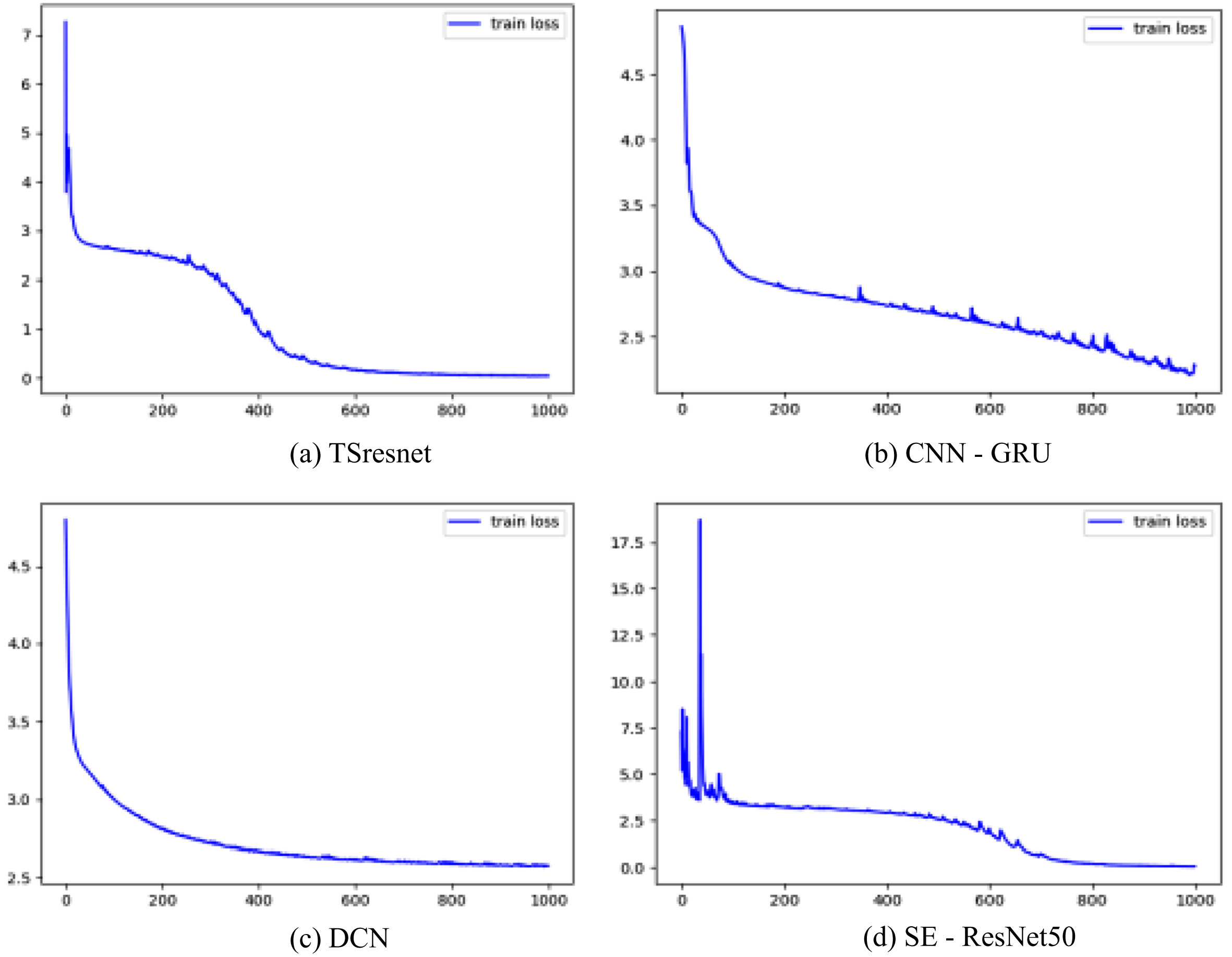
Loss function plot.

Table 3

Network parameter

Name
Epoch	1000
Learning rate	0.0007
Optimizer	SGD
Loss function	CrossEntropyLoss

According to the experimental results, the CNN-GRU network cannot further reduce its loss value due to insufficient time series feature extraction ability in figure (b). Figure (c) DCN network is unable to extract deep data features due to its own system depth limitation resulting in its high loss. Figure (d) the SE-ResNet50 network, although very capable of extracting deep information, is not as stable as the TSresnet network. The TSresnet method used in this paper is shown in Figure (a), which proves that TSresnet can better deal with deep feature problems and has better robustness from three levels of vibration amplitude, loss value and stability.

3.4.2 Performance evaluation experiment

The performance effects of four different networks are shown in Table 4:

Table 4
Performance comparison on C-MAPSS dataset

Network FD001 FD002 FD003 FD004

TSresnet RMSE 30.92 33.94 30.98 40.63

SCORE 3913 6426 2419 10558

R-squared 0.50 0.47 0.44 0.40

CNN-GRU RMSE 36.87 36.01 33.38 39.43

SCORE 5073 8465 8240 11148

R-squared 0.22 0.51 0.39 0.44

DCN RMSE 37.12 37.49 37.12 45.32

SCORE 6018 13982 7670 23786

R-squared 0.21 0.50 0.32 0.31

SE-ResNet50 RMSE 38.10 39.61 38.72 40.89

SCORE 6957 9119 10498 10646

R-squared 0.25 0.45 0.38 0.33

Network		FD001	FD002	FD003	FD004
TSresnet	RMSE	30.92	33.94	30.98	40.63
	SCORE	3913	6426	2419	10558
	R-squared	0.50	0.47	0.44	0.40
CNN-GRU	RMSE	36.87	36.01	33.38	39.43
	SCORE	5073	8465	8240	11148
	R-squared	0.22	0.51	0.39	0.44
DCN	RMSE	37.12	37.49	37.12	45.32
	SCORE	6018	13982	7670	23786
	R-squared	0.21	0.50	0.32	0.31
SE-ResNet50	RMSE	38.10	39.61	38.72	40.89
	SCORE	6957	9119	10498	10646
R-squared	0.25	0.45	0.38	0.33

From the table, it can be seen that TSresnet network has significant advantages over CNN-GRU network, DCN network, SE-ResNet50 network, on FD001 and FD002 datasets, TSresnet still has advantages in RMSE and SCORE, although some metrics are inferior to other networks. In the FD003 dataset, TSresnet has a significant advantage in all three metrics, with SCORE being 71%, 68% and 77% lower than the other networks respectively. On the FD004 dataset, the performance of the four networks has decreased, this is because the data situation is more complex in FD004, there are six working states and two failure modes. FD004 is recognized as the most difficult dataset for life prediction. However, it still has certain advantages in the SCORE. Overall, TSresnet performs well on the four sub-data sets, which means that TSresnet is better at extracting time-series features and processing complex data and can predict the remaining engine life more accurately.

To demonstrate the network performance, the experimental results in published papers are compared on the FD002 and FD004 datasets, as shown in Tables 5 and 6:

Table 5

Performance comparison of FD002

FD002	DBN [29]	ELM [29]	CNN [30]	TSresnet
RMSE	27.12	37.28	30.29	33.94
SCORE	9031	498149	13570	6426

Table 6

Performance comparison of FD004

FD004	MLP [30]	SVR [30]	RVR [30]	TSresnet
RMSE	77.36	45.35	34.34	40.63
SCORE	5616600	371140	26509	10558

It can be seen that whether in FD002 or FD004, TSresnet performs better on SCORE than other methods, which indicates that it has higher commercial value in remaining useful life prediction.

3.4.3 Single aero-engine life prediction

Engine 01 in FD001 is selected for life prediction display, and the experimental results are shown in Fig. 10, where (a) is TSresnet network, (b) is CNN-GRU network, (c) is DCN network, and (d) is SE-ResNet50 network.

Fig. 10

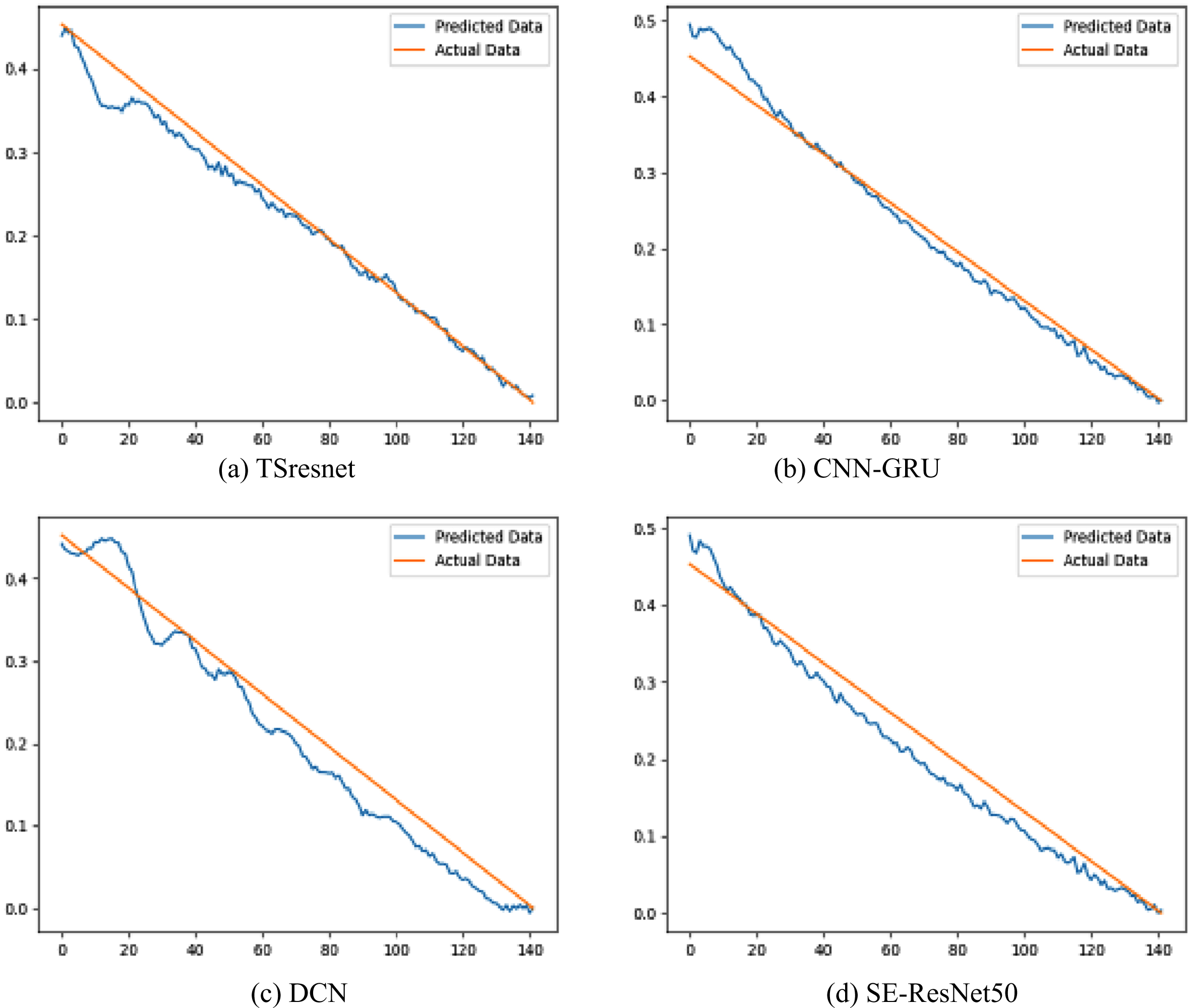
Life prediction of engine 01.

It can be found that the fluctuations in the early prediction stages of all four networks are large, which is caused by the lack of obvious degradation characteristics at the beginning of operation, and as the aero-engine continues to operate, its degradation characteristics become more and more obvious, and the most accurate prediction is made close to failure. In an industrial context, if engine health and remaining life can be accurately predicted in the early stages of operation, the more significant it will be in engineering practice. TSresnet enables accurate prediction of remaining life in the mid-operation phase with a better fit and less oscillation, which makes it of high industrial value.

3.4.4 Ablation experiments

The experiments compare the experimental effects of removing the time-series feature extraction layer and removing the deep feature extraction layer on dataset FD001 separately, using three performance evaluation metrics to show the impact of the missing part on the network performance respectively. Figure 11 shows the RMSE comparison, Fig. 12 shows the SCORE comparison, and Fig. 13 shows the R-squared comparison.

Fig. 11

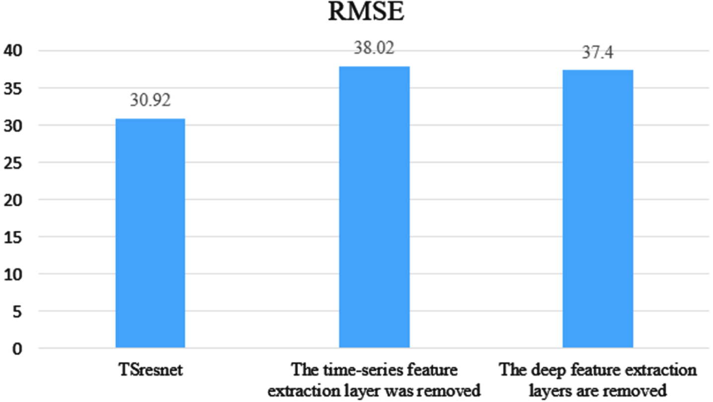
RMSE comparison.

Fig. 12

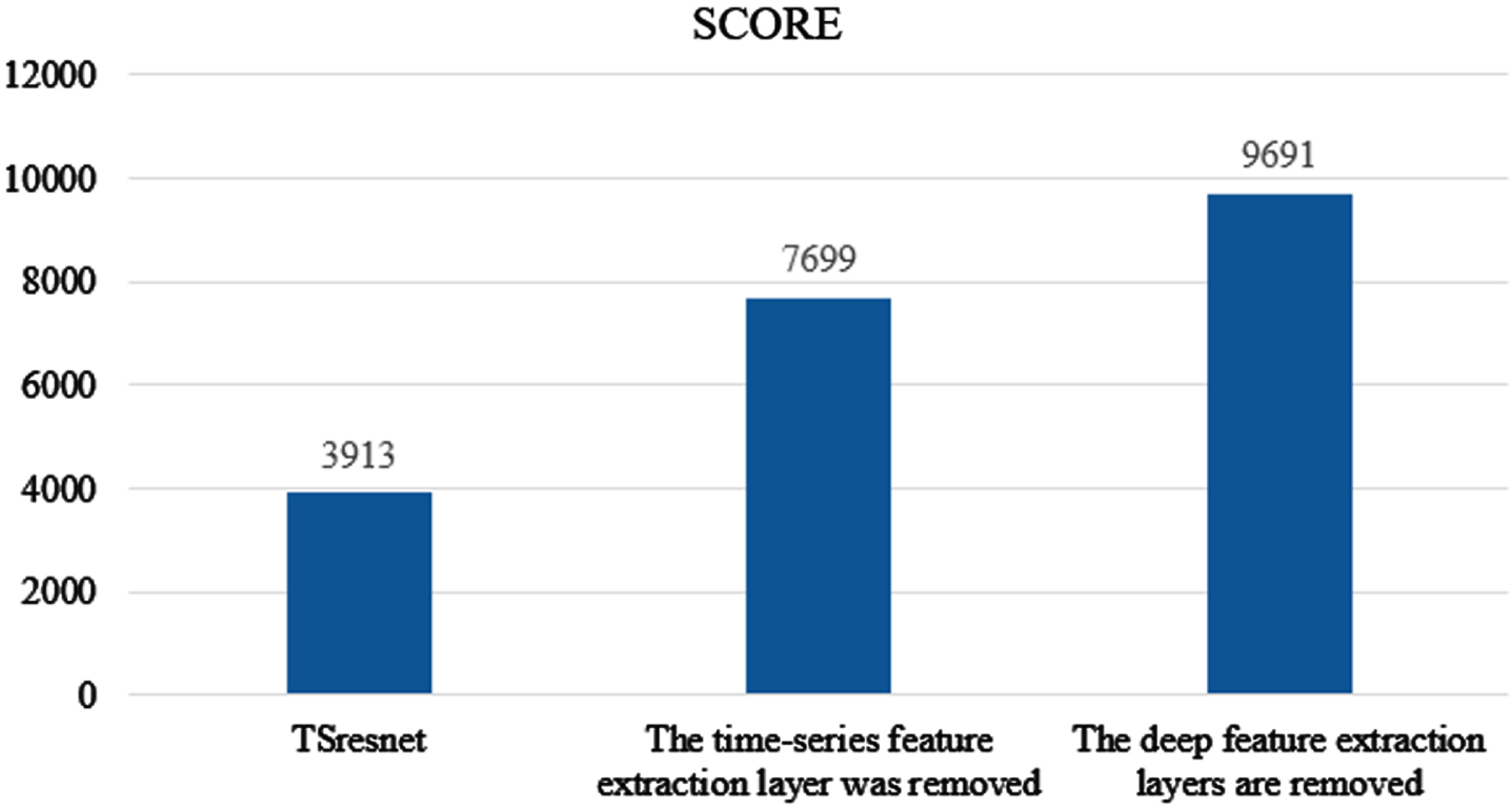
SCORE comparison.

Fig. 13

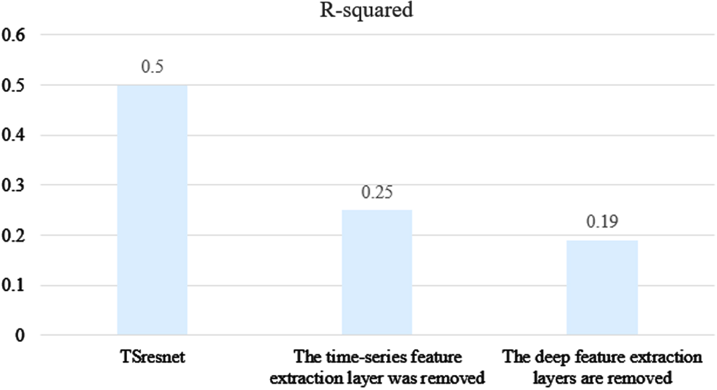
R-squared comparison.

From Figs. 11 to 13 it can be seen that TSresnet obtains better results in terms of the evaluation metrics when comparing the two networks with the removal of the time-series feature extraction layer and the removal of the deep feature extraction layer. Among them, the SCORE is 49% and 59% lower than the other two groups of experiments, which shows that TSresnet can achieve better results in advance prediction. The R-squared was 100% and 163% higher than the remaining two groups respectively, indicating that TSresnet predicted the remaining life more closely to its true life under the complex condition of multiple feature inputs and the network fit was better.

4 Conclusion

TSresnet is proposed for the remaining life prediction of aero engines, and the structural design of the network model and the corresponding calculation methods are described in detail. The time series feature extraction layer through the three-head structure breaks through the constraints of the traditional network on the convolution kernel, solves the interference of complex data on the network through the addition of the attention mechanism, and solves the problem that it is difficult to extract deep features through the deep feature extraction layer. The test results on the C-MAPSS aero-engine dataset provided by NASA show that the network model proposed in this paper has strong ability to process time series features and deep features, and can predict the remaining life of the engine more accurately. Therefore, it shows that the network model proposed in this paper can solve the problems caused by too large data sets, and has excellent performance, which also shows that the network has high industrial value.

Footnotes

Acknowledgments

This work is supported in part by the National Natural Science Foundation of China (No. 62241307), the Key Research and Development Program of Science and Technology Department of Gansu Province (No. 22YF7FA166), the Scientific and Technological Project of Lanzhou City (No. 2022-RC-60) and the University Innovation Fund Project of Gansu Province (No. 2021A-027).

References

Salfner

Felix

, Lenk

Maren

and Malek

Miroslaw

, A survey of online failure prediction methods, ACM Computing Surveys (CSUR) 42(3) (2010), 1–42.

Zhang

, et al., Automated IT system failure prediction: A deep learning approach, 2016 IEEE International Conference on Big Data (Big Data), IEEE, 2016.

Jin

Xin

, et al., Failure prediction, monitoring and diagnosis methods for slewing bearings of large-scale wind turbine: A review, Measurement 172 (2021), 108855.

Wang

Youdao

, Zhao

Yifan

and Addepalli

Sri

, Remaining useful life prediction using deep learning approaches: A review, Procedia Manufacturing 49 (2020), 81–88.

Zhao

Huimin

, et al., Feature extraction for data-driven remaining useful life prediction of rolling bearings,, IEEE Transactions on Instrumentation and Measurement 70 (2021), 1–10.

Cheng

Han

, et al., Transferable convolutional neural network based remaining useful life prediction of bearing under multiple failure behaviors, Measurement 168 (2021), 108286.

Qin

, et al., Gated dual attention unit neural networks for remaining useful life prediction of rolling bearings, IEEE Transactions on Industrial Informatics 17(9) (2020), 6438–6447.

Meng

and Mao

Zhu

, Deep-convolution-based LSTM network for remaining useful life prediction, IEEE Transactions on Industrial Informatics 17(3) (2020), 1658–1667.

Naipeng

, et al., Remaining useful life prediction based on a multi-sensor data fusion model}, Reliability Engineering & System Safety 208 (2021), 107249.

10.

Wen

Pengfei

, et al., A generalized remaining useful life prediction method for complex systems based on composite health indicator, Reliability Engineering & System Safety 205 (2021), 107241.

11.

Xiang

, Zhang

Wei

and Ding

Qian

, Deep learning-based remaining useful life estimation of bearings using multi-scale feature extraction, Reliability Engineering & System Safety 182 (2019), 208–218.

12.

Liu

Kailong

, et al., A data-driven approach with uncertainty quantification for predicting future capacities and remaining useful life of lithium-ion battery, IEEE Transactions on Industrial Electronics 68(4) (2020), 3170–3180.

13.

Wang

Jinjiang

, et al., An integrated fault diagnosis and prognosis approach for predictive maintenance of wind turbine bearing with limited samples, Renewable Energy 145 (2020), 642–650.

14.

Ren

Lei

, et al., Remaining useful life prediction for lithium-ion battery: A deep learning approach, IEEE Access 6 (2018), 50587–50598.

15.

Ren

Lei

, et al., Bearing remaining useful life prediction based on deep autoencoder and deep neural networks, Journal of Manufacturing Systems 48 (2018), 71–77.

16.

Wang

Biao

, et al., A hybrid prognostics approach for estimating remaining useful life of rolling element bearings, IEEE Transactions on Reliability 69(1) (2018), 401–412.

17.

Jiuxiang

, et al., Recent advances in convolutional neural networks, Pattern Recognition 77 (2018), 354–377.

18.

Lavin

Andrew

and Gray

Scott

, Fast algorithms for convolutional neural networks, Proceedings of the IEEE conference on computer vision and pattern recognition, 2016.

19.

Kiranyaz

Serkan

, et al., 1D convolutional neural networks and applications: A survey, Mechanical systems and signal processing 151 (2021), 107398.

20.

Hewage

Pradeep

, et al., Temporal convolutional neural (TCN) network for an effective weather forecasting using time-series data from the local weather station, Soft Computing 24(21) (2020), 16453–16482.

21.

Wang

Yuanyuan

, et al., Short-term load forecasting for industrial customers based on TCN-LightGBM, IEEE Transactions on Power Systems 36(3) (2020), 1984–1997.

22.

Woo

Sanghyun

, et al., Cbam: Convolutional block attention module, Proceedings of the European conference on computer vision (ECCV) 2018.

23.

Liang

Gaobo

and Zheng

Lixin

, A transfer learning method with deep residual network for pediatric pneumonia diagnosis, Computer Methods and Programs in Biomedicine 187 (2020), 104964.

24.

Asif

Owais

, et al., A Deep Learning Model for Remaining Useful Life Prediction of Aircraft Turbofan Engine on C-MAPSS Dataset, IEEE Access 10 (2022), 95425–95440.

25.

Wang

Pingfeng

, Youn

Byeng D.

and Hu

Chao

, A generic probabilistic framework for structural health prognostics and uncertainty management, Mechanical Systems and Signal Processing 28 (2012), 622–637.

26.

Wei

Yang

, et al., Transformer short-term fault prediction method based on CNN-GRU combined neural network, Power System Protection and Control 50(6) (2022), 107–116.

27.

Yanfei

, et al., Bayesian optimized deep convolutional network for bearing diagnosis, The International Journal of Advanced Manufacturing Technology 108(1) (2020), 313–322.

28.

Theckedath

Dhananjay

and Sedamkar

R.R.

, Detecting affect states using VGG16, ResNet50 and SE-ResNet50 networks, SN Computer Science 1(2) (2020), 1–7.

29.

Zhang

Chong

, et al., Multiobjective deep belief networks ensemble for remaining useful life estimation in prognostics, IEEE Transactions on Neural Networks and Learning Systems 28(10) (2016), 2306–2318.

30.

Babu

Giduthuri Sateesh

, Zhao

Peilin

and Li

Xiao-Li

, Deep convolutional neural network based regression approach for estimation of remaining useful life, International conference on database systems for advanced applications, Springer, Cham, 2016.

Aero-engine residual life prediction based on time-series residual neural networks

Abstract

Keywords

1 Introduction

2 Residual life prediction model based on time-series residual networks

2.1 Time-series feature extraction layer

3.1 The C-MAPSS dataset

Table 2 C-MAPSS dataset C-MAPSS FD001 FD002 FD003 FD004 Number of training sets 100 260 100 249 Number of test sets 100 259 100 248 Working condition 1 6 1 6 Failure mode 1 1 2 2 Train sample 17731 48819 21820 57522 Test sample 100 259 100 248

3.4.1 Loss function comparison experiment

Footnotes

Acknowledgments

References

Table 2
C-MAPSS dataset

C-MAPSS

FD001 FD002 FD003 FD004

Number of training sets 100 260 100 249

Number of test sets 100 259 100 248

Working condition 1 6 1 6

Failure mode 1 1 2 2

Train sample 17731 48819 21820 57522

Test sample 100 259 100 248