A novel energy consumption prediction method for chillers based on an improved support vector machine

Abstract

The energy consumption prediction of the chiller is an important means to reduce the energy consumption of buildings. Therefore, a novel energy consumption prediction model for chillers based on an improved support vector machine (ICA-DE-SVM) is proposed. The imperialist competitive algorithm (ICA) is used to optimize the penalty coefficient and kernel function width of SVM, greatly improving the generalization ability and prediction accuracy of the SVM model. The assimilation process is very important in ICA. Colonies of empires move randomly toward imperialists during the assimilation process in ICA, which decreases population diversity and can lead to premature convergence. Therefore, to create more new locations for colonies and increase population diversity, the idea of differential mutation proposed by differential evolution (DE) was applied to ICA. The established model was experimentally verified in an actual multi-chiller system in a building, and the results showed that the ICA-DE-SVM model could obtain good prediction results. Finally, the proposed model was compared with SVM model, PSO-SVM model, GA-SVM model, WOA-SVM model, and ICA-SVM model. With an MAPE of 0.6%, an MSE of 2.3, and an R² of 0.9998, the findings demonstrate that the ICA-DE-SVM model has a greater prediction accuracy than the other models.

Keywords

Energy consumption prediction imperialist competitive algorithm Chillers support vector machine

1 Introduction

Achieving carbon peak and carbon neutrality is a broad and profound socio-economic transformation. The proposed “double carbon” goal has elevated the green development path to a new height. Energy consumption is the key to achieving “double carbon” [1].

The central air-conditioning system of the whole building is the highest energy consuming facility, and its power consumption accounts for a large part of the total power consumption of the building. The cold source system is one of the main components of the central air conditioner, and it consumes a lot of energy. Therefore, the energy consumption optimization of the cold source system is an important means to reduce the energy consumption of buildings. However, due to the nonlinear, hysteretic, complex operating, time-varying and strong coupling conditions of the cold source system, its actual energy consumption optimization is costly and time-consuming. Therefore, establishing the model of energy consumption prediction of the cooling source system and realizing the energy consumption prediction under different working conditions is one of the important ways to achieve energy conservation in buildings [2, 3].

The energy consumption prediction method of the cold source system is separated into 3 main categories. The first category is a physical model based on thermodynamic mechanisms, the second category is a gray box model using mechanism information modeling, and the third category is a data-driven black box model [4]. The physical model requires a lot of information, which results in the establishment of its thermodynamic model. The physical model is usually reliable and reflects the operation of the device. However, the establishment of a physical model requires knowledge of a large amount of information and consumes a lot of human and material resources. The gray box model consists of building the structure of the model by analyzing the information of the device and then identifying the parameters of the model through operation data of equipment [5]. Afram A et al. [6] identified the parameters of the energy consumption model of chillers through the experimental data. Janabi-Sharifi F et al. [7] established the grey box model of the cooling tower, and verified the usefulness and adaptability of the grey box model through experiments. The grey box model is more accurate than the physical model, but it needs to keep a lot of information of the machine operation yet.

In the past, regression models were mainly used to forecast energy consumption by scholars [8 –12]. Due to the rapid development of machine learning, it is more and more widely used in the field. Kim J-H et al. [13] established the energy consumption prediction model of the cold source system by using multilayer perceptron (MLP), and verified the effectiveness of the model. Li et al. [14] proposed a new neural network structure with an attention mechanism based on building energy consumption prediction of the RNN model. Wang et al. [15] established the power consumption prediction method by using the extreme value gradient lifting, and carried out a comparative test between the models established.

Su et al. [16] suggest a unique capacity prediction approach for SOH estimates based on deep learning, transfer learning, and the battery equivalent circuit model. Su et al. [17] provide a capacity estimation approach for an adaptive boosting charging strategy that is utilized for state estimation and adaptive charging strategy modification during the charging and discharging cycle process. Black-box data-driven models have been utilized extensively, but their precision is primarily dependent on the caliber and number of learning samples. The sample data in the actual field are frequently accompanied by noise, which has a negative impact on the data-driven model. In addition, many essential data describing the operating characteristics of the object are difficult to gather directly in the actual process. The generalization capacity of the model decreases dramatically when the system’s operational conditions change or the learning samples’ coverage is limited [18].

Due to the nonlinear, hysteretic, complex operating, time-varying, and strong coupling conditions of the cold source system, its actual energy consumption optimization is costly and time-consuming. These conclusions motivated us to investigate more effective machine learning techniques. In the rest of this paper, we present our method as well as a reference implementation for dealing with energy consumption prediction for chillers.

Support vector machine (SVM) is based on kernel function theory, which maps samples to high dimensional space and has unique advantages in dealing with small samples, high-dimensional, nonlinear problems. Zhao et al. [19] compared the SVR model with the ANN model and GPR model, and verified the usefulness and adaptability of the SVR method through experiments. Tang et al. [20] established an SVR model according to the selected input variables. They then used the office building’s data set to confirm the model’s efficacy. The SVM approach was used by Paudel et al. [21] to forecast how much energy a university would use. The choice of the penalty parameters and kernel function parameters, however, has a significant impact on the prediction performance of an SVM model in practice. Many swarm intelligence optimization algorithms, such as the genetic algorithm, particle swarm optimization, cuckoo search algorithm (CSA), and others, have been applied to SVM parameter optimization. Jing W et al. [22] proposed a energy-saving diagnosis method based on an enhanced PSO-SVM model. Ding Y et al. [23] established prediction models for office buildings based on the GA-SVR and GA-WD-SVR algorithms. However, these optimization algorithms have some flaws, such as being prone to local optimums, taking a long time to run, providing insufficient feedback information, and failing to achieve optimal prediction performance.

The imperialist competitive algorithm (ICA) proposed by Atashpaz Gargari and Lucas in 2007 [24], is a socially inspired randomized and optimized search method. Currently, ICA has been effectively used to solve a variety of optimization issues such as scheduling, classification and mechanical design [25, 26]. In an experimental comparison of published literature, when compared to other algorithms, ICA has better local and global search capabilities, faster convergence speed, and tolerable calculation times (e.g., GA, PSO, etc.) [27, 28]. In ICA, the differential mutation idea of DE algorithm is used to improve the assimilation process of ICA in order to improve the diversity of solutions generated in the assimilation process and increase the probability of jumping out of the local optimal solution. The new algorithm is called ICA-DE.

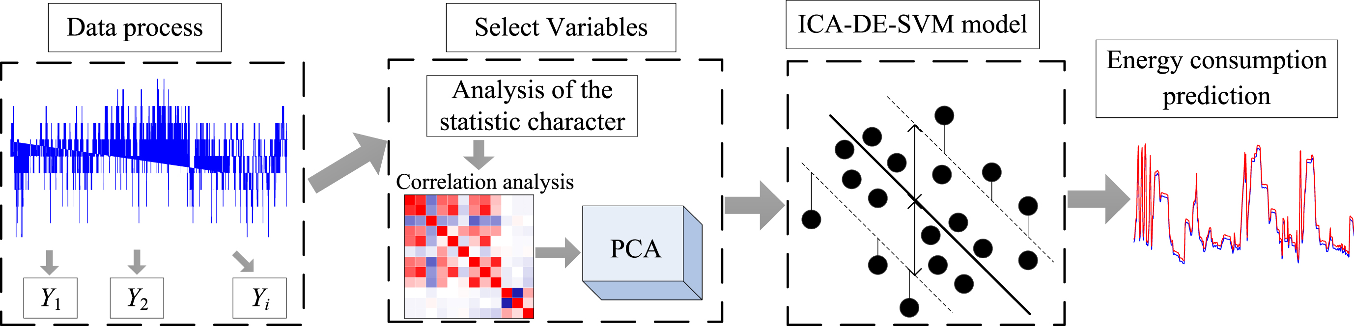
The ICA-DE is used to optimize the penalty coefficient and kernel function width of SVM and establish an energy consumption prediction model for chillers based on the ICA-DE-SVM model. The proposed model is experimentally verified in an actual building. The experimental results show that the ICA-DE-SVM model has a better effect than the other methods. The overall idea of this article is shown in Fig. 1. The main innovations are as follows:

A novel energy consumption prediction method for chillers based on ICA-DE-SVM is proposed. The established model was experimentally verified in the actual building, and the results showed that the ICA-DE-SVM method could obtain good prediction results;

The proposed ICA-DE differs from the original ICA in that it allows colonies to learn not only from their corresponding imperialists but also from other colonies in the empire. This decreases the possibility of trapping in the local optimum and increases the chance of finding a better position;

Apply the differential mutation idea that was proposed by differential evolution (DE) to ICA. In ICA-DE, the mutation rate and crossover ratio are not always constant but vary with the evolution process, which can improve the convergence speed of the algorithm.

Fig. 1

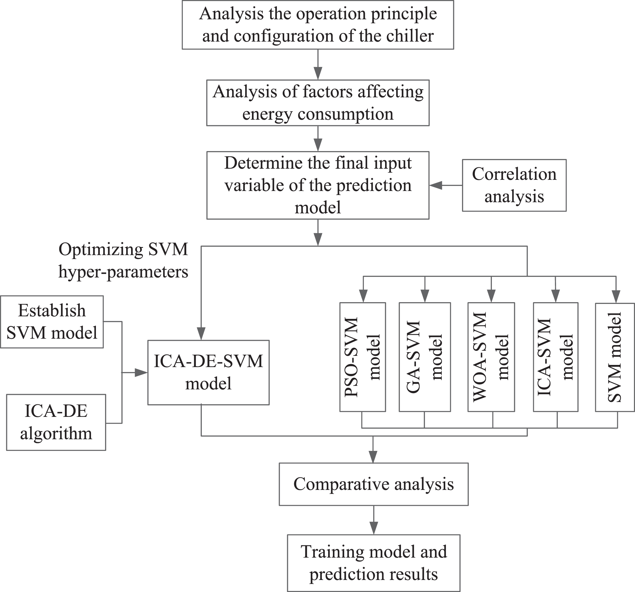
The flow chart of overall thought.

The paper is arranged as follows: Section 2 introduces the composition and working principle of the cold source system, and analyzes the main factors that affect the energy consumption of chillers. In Section 3, the ICA-DE-SVM model is constructed, and the process of using the model to predict energy consumption is introduced. Section 4 experimentally verifies the usefulness and adaptability of the model proposed in this article and compares it with other methods. Section 5 gives the conclusion and an outlook for future work.

2 Analysis of influencing factors

2.1 The operation principle and configuration of the chiller

As shown in Fig. 2, the chiller is mainly composed of four parts, namely compressor, expansion valve, evaporator and condenser.

Fig. 2

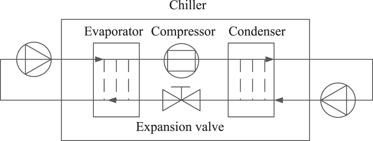
The configuration of chillers.

As shown in Fig. 3, the three primary cycles in the cold source system are the refrigerant cycle, the chilled water cycle, and the cooling water cycle. The purpose of the refrigerant cycle is to complete the heat transfer from chilled water to cooling water. In the refrigerant cycle’s evaporator, the refrigerant evaporates, absorbs heat, and then releases heat from the chilled water. A significant amount of heat is released into the cooling water as the refrigerant condenses in the condenser, and this heat is then carried by the cooling tower to the outside air. The compressor converts low temperature, low pressure gas refrigerant into high temperature, high pressure gas refrigerant. In the expansion valve, the high-temperature, high-pressure liquid refrigerant is changed into a low-temperature, low-pressure refrigerant. In addition to completing interior temperature and humidity adjustments, chilled water circulation serves to remove heat generated in the space and maintain a cool environment. Through terminal devices like fan coil units, the low-temperature chilled water transfers heat to the indoor air and removes it. The purpose of cooling water circulation is to dissipate heat into the atmosphere, bringing down the temperature of the cooling water. High-temperature cooling water enters the cooling tower, where it exchanges heat with the ambient air to transform into low-temperature cooling water. Returning to the condenser, the low-temperature cooling water continues to collect heat and transforms into high-temperature cooling water.

Fig. 3

The operation principle of chillers.

2.2 Determination of input variables

The factors affecting the energy consumption of chillers are very complex, which are not only affected by each facility, but also by working environment. Based on a review of the cold source system’s operating mechanism, the main factors affecting the energy consumption of chillers can be preliminary determined, as shown in Fig. 4 and Table 1.

Fig. 4

Influencing factors: (a) influencing factors in chilled water cycle and (b) influencing factors in cooling water cycle.

Table 1

Variables affecting energy consumption

Variable’s name	Meaning of variables
T _h1	Supply temperature of chilled water
T _h2	Return temperature of chilled water
Q _ch	Chilled water flow rate
Q _cl	Cooling water flow rate
T _c1	Supply temperature of cooling water
T _c2	Return temperature of cooling water
COP	Coefficient of performance
W	Cooling capacity of chillers
PLR	Partial load rate of chillers
T ₀	Outdoor temperature
T _hu	Humidity
T _wb	Wet bulb temperature

As shown in Table 1, the T_h1, T_h2, Q_ch, Q_cl, T_c1, T_c2, COP, W, PLR, T_0, T_hu, and T_wb are used as input variables to establish a model for predicting the energy consumption of chillers.

3 Establishment model

To better understand the ICA-DE-SVM model, in Section 3.1, the basics of ICA are introduced. In Section 3.2, the ICA-DE method is introduced, and then the ICA-DE-SVM model is detailed in Section 3.3.

3.1 ICA

(a) Initialization

In ICA, each individual is referred to as a country. In solving the optimization problem, each group of solutions is called a country. Each element in a country corresponds to each variable of the optimization problem. For a D-dimensional optimization problem, the i-th country can be expressed as follows:

$\begin{matrix} {country}_{i} = X_{i} \\ = [x_{i 1}, x_{i 2}, \dots, x_{iD}], i = 1, 2, \dots, N \end{matrix}$ (1)

The power of a country is expressed as a cost function, and the cost of the i-th country is expressed as: ${cost}_{X_{i}} = f ({country}_{i})$ (2) where f (·) is the objective function of the optimization problem. The power of a country is inversely proportional to its cost.

N countries are randomly generated, and the elements of each country are generated as: $x_{ij} = {lb}_{j} + ({ub}_{j} - {lb}_{j}) \times rand (•), j = 1, 2, \dots, D$ (3) where rand is a uniform random number that takes values from 0 to 1. x_ij is the j-th dimensional variable for the i-th country X_i. lb_j is the lower limit of the j-th dimensional variable under constraint conditions, and ub_j is the upper limit of the j-th dimensional variable under constraint conditions.

The cost of the randomly generated N countries is calculated and then the first N_imp countries that are powerful are chosen as imperialist and the rest of the N_col countries as colonies. The colonies are distributed according to the size of the imperialist power. The greater the power, the more colonies are distributed, and the smaller the power, the fewer colonies are distributed. The number of colonies owned by each imperialist is calculated as follows [27]: ${Power}_{n} = | \frac{C_{n}}{\sum_{i = 1}^{N_{imp}} C_{i}} |$ (4) $C_{n} = {cost}_{X_{n}} - max_{i} {{cost}_{X_{i}}}$ (5) ${NC}_{n} = round {{Power}_{n} \times N_{col}}$ (6) where C_n is the normalized cost of the cost_{X
_n}, Power_n is the normalized power of the i-th imperialist, and NC_n is the quantity of colonies. The N_col colonies are randomly distributed to the imperialists according to the calculation results. N_imp empires were finally formed, as shown in Fig. 5.

Fig. 5

The empire.

(b) Assimilation

In the process of assimilation, all colonies of the empire shifted to imperialism. The inclination between the moving direction and the connecting direction of the colony and imperialist is θ, as shown in Fig. 6. θ is a uniformly distributed random number, which can be expressed as [30]:

Fig. 6

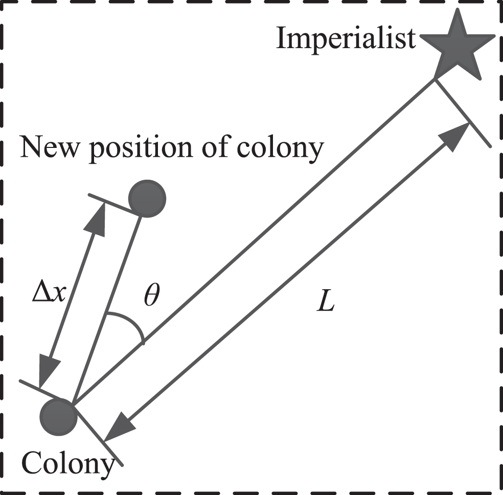
The process of assimilation.

$θ \sim U (- γ, γ)$ (7) where γ is the assimilation angle coefficient, usually γ = π/4 [22].

The current position of the i-th colony is X_i, and the new position after moving can be expressed as: $X_{NEWi} = X_{i} + Δ x_{i}$ (8) where Δx_i is a uniformly distributed random variable, which can be expressed as: $Δ x_{i} \sim U (0, β \times L)$ (9) where L is the distance between the colony and imperialist to which it belongs, and β is the assimilation coefficient, β = 2.

In the assimilation process, when a colony moves to a new position, if its cost is less than the imperialist to which it belongs, that is, if its power is greater than that of the imperialist to which it belongs, the positions between the colony and its imperialist should be exchanged; in other words, the colony becomes an imperialist in the empire, while the original imperialist becomes a colony [31], as shown in Fig. 7.

Fig. 7

Exchange positions between colony and imperialist.

(c) Imperialistic competition

Empire competition is the process by which the stronger empire occupies the colony of the weaker empire [32]. The first step is to calculate the total cost of empire, that is, the size of empire power. Imperialist has a great influence on the whole empire, while the influence of colonies is very small. Therefore, ICA calculates the total cost of the n-th empire using the following formula:

${TC}_{n} = {cost}_{n}^{X_{imp}} + ξ \times \frac{\sum_{i = 1}^{{NC}_{n}} {cost}_{n}^{X_{coli}}}{{NC}_{n}}$ (10) where ξ is the cost ratio coefficient, 0 < ξ < 1. The size of ξ determines the influence of colonies on the whole empire. In this paper, ξ = 0.5. ${cost}_{n}^{X_{imp}}$ is the cost of imperialist in the n-th empire and ${cost}_{n}^{X_{coli}}$ is the cost of the i-th colony in the n-th empire. The weakest colony from the weakest empire is chosen as the object of empire competition. The stronger the empire, the greater the probability of occupying a colony. The occupancy probability of the n-th empire is defined as:

$p_{n} = | \frac{{NTC}_{n}}{\sum_{j = 1}^{N_{imp}} {NTC}_{j}} |, n = 1, 2, \dots, N_{imp}$ (11) ${NTC}_{n} = {TC}_{n} - max_{i} {{TC}_{i}}$ (12) where NTC_n is the normalized cost of the n-the empire. The competitive process is shown in Fig. 8.

Fig. 8

Competitive process.

(d) Elimination of powerless imperialists

By occupying the colonies of other empires, powerful empires became increasingly powerful, while the number of colonies of the weaker empire declined. If an empire loses every colony, that empire is wiped out [33]. With the elimination of empires, one empire is finally left. At this time, the algorithm terminates.

3.2 ICA-DE

In ICA, the assimilation process is very important. It explores the optimal solution to the optimization problem. In each empire, colonies move in order to create a better position and thus increase the total power of the empire. However, the movement of colonies to imperialist in the assimilation process of ICA is random, which reduces the diversity of the population and can lead to premature convergence. Therefore, in order to create more new locations for colonies and increase population diversity, the idea of differential mutation proposed by differential evolution was introduced into ICA. The new algorithm is called ICA-DE. The assimilation process of the new algorithm is shown in Fig. 9.

Fig. 9

The process of mutation and crossover.

The colony X_coli in an empire generates a mutation position, which is expressed as: $X_{coli}^{mut} = X_{imp} + F \times (X_{col 1} - X_{col 2})$ (13) where X_imp represents the imperialist in the empire at the current iteration, and X_col₁ and X_col₂ are any two colonies of the empire. F is the mutation rate, denoted as: $F = F_{min} + (F_{max} - F_{min}) \times \frac{{cost}_{X_{col 1}} - {cost}_{X_{imp}}}{{cost}_{X_{col 2}} - {cost}_{X_{imp}}}$ (14) where F_max represents the maximum value of F and F_min represents the minimum value of F. F_max = 0.9 and F_min = 0.1. To further improve the diversity of imperialist countries, crossover operations are constantly carried out. The position after the crossover operation $X_{coli}^{cross}$ can be expressed as: $X_{coli}^{cross} = [x_{coli 1}^{cross}, x_{coli 2}^{cross}, \dots, x_{coliD}^{cross}]$ (15) $X_{coli}^{mut} = [x_{coli 1}^{mut}, x_{coli 2}^{mut}, \dots, x_{coliD}^{mut}]$ (16) $X_{coli} = [x_{coli 1}, x_{coli 2}, \dots, x_{coliD}]$ (17) $x_{colij}^{cross} = {\begin{matrix} x_{colij}^{mut}, rand (•) < CR \\ x_{colij}, rand (•) ⩾ CR \end{matrix}, j = 1, 2, \dots, D$ (18) where CR denotes the crossover ratio, which can be expressed as: $\begin{matrix} CR = {CR}_{min} + ({CR}_{max} - {CR}_{min}) \times \\ \frac{{cost}_{X_{coli}} - {cost}_{X_{weakest}}}{cos t_{X_{imp}} - cos t_{X_{weakest}}} \end{matrix}$ (19) where CR_max represents the maximum value of CR and CR_min represents the minimum value of CR. In this paper, we set CR_max = 0.6 and CR_min = 0.1. cost_{X
_weakest} is the cost of the weakest colony X_weakest in the empire_. The final position $X_{coli}^{'}$ of the X_coli in the empire after the crossover operation is expressed as: $X_{coli}^{'} = {\begin{matrix} X_{coli}^{cross} {cost}_{X_{coli}^{cross}} < {cost}_{X_{coli}} \\ X_{coli} {cost}_{X_{coli}^{cross}} ⩾ {cost}_{X_{coli}} \end{matrix}$ (20)

The F and CR can improve the exploration ability of the new algorithm, but the capacity for exploitation will decline in tandem. Two iterative indicators I₁ and I₂ are set to regulate when the mutation and crossover alter adaptively in order to achieve a better balance between exploration and exploitation. Algorithm 1 illustrates the new assimilation process.

Algorithm 1 The assimilation process of ICA-DE
Input: The imperialist X_imp and colonies X_coli;
The worst colonies X_weakest;
The number of colonies N_col;
The maximum iteration number I_max;
Output: The X_imp, X_i and X_weakest;
1:fori = 1 to N_coldo
2: ifI< = I₁then
3: $CR = 0.1 + 0.5 \times \frac{{cost}_{X_{coli}} - {cost}_{X_{worst}}}{cos t_{X_{imp}} - cos t_{X_{weakest}}}$
4: else
5: CR = 0.9
6: end if
7:col1 = rand(N_col)
8: col2 = rand(N_col)
9: ifI< = I₂then
10: $F = 0.1 + 0.8 \times \frac{{cost}_{X_{col 1}} - {cost}_{X_{imp}}}{{cost}_{X_{col 2}} - {cost}_{X_{imp}}}$
11: else
12: F = 0.5
13: end if
14: $X_{coli}^{mut} = X_{imp} + F \times (X_{col 1} - X_{col 2})$
15: forj = 1 to ddo
16: if rand(.) < CR then
17: $x_{colij}^{cross} = x_{colij}^{mut}$
18: else
19: $x_{colij}^{cross} = x_{colij}$
20: end if
21:end for
22: if ${cost}_{X_{coli}^{cross}} < {cost}_{X_{coli}}$ then
23: $X_{coli} = X_{coli}^{cross}$
24:end if
25: else
26: $X_{imp} = X_{coli}^{cross}$
27: end if
28:end for

3.3 ICA-DE-SVM

The prediction impact of SVM is superior to the present ELM and BP neural networks, whose energy consumption is influenced by too many parameters. As a result, the SVM is employed to create an energy consumption prediction model for chillers.

A set of input and output data sets, it can be represented as: $Y = {[(x_{11}, \dots, x_{1 n}), y_{1} (x_{11}, \dots, x_{1 n})], \dots, [(x_{m 1}, \dots, x_{m n}), y_{m} (x_{m 1}, \dots, x_{m n})]}$ (21) where x_mn is the input variable, y_m is the energy consumption of chillers, n is the number of variables, m is the number of samples. The regression function model of the SVM is expressed as [34]: $y_{m} (x_{m 1}, \dots, x_{mn}) = ω \cdot φ (x_{m 1}, \dots, x_{mn}) + b$ (22) where ω is the hyper plane coefficient, b is the undetermined offset, φ (•) is an unknown high-dimensional function, and ω · φ (x_m1, ⋯ , x_mn) is the inner product of ω and φ (x_m1, ⋯ , x_mn).

It is necessary to solve for the coefficients ω and b in order to obtain the nonlinear fitting function depicted in Equation (22). By including relaxation variables ξ_i ( $ξ_{i}^{*} ⩾ 0$ ), Equation (22) can be transformed into the following optimization problem in accordance with the theory of support vector machine regression [35]: $\begin{matrix} min_{ω, b, ξ} {\frac{1}{2} | | ω | |^{2} + c \sum_{i = 1}^{m} (ξ_{i} + ξ_{i}^{*})} \\ s . t . y_{m} (x_{m 1}, \dots, x_{mn}) - ω \cdot φ (x_{m 1}, \dots, x_{mn}) \\ - b ⩽ ɛ + ξ_{i} - y_{m} (x_{m 1}, \dots, x_{mn}) + ω \cdot φ (x_{m 1}, \\ \dots, x_{mn}) + b ⩽ ɛ + ξ_{i}^{*} (i = 1, 2, \dots, m) . \end{matrix}$ (23) where $c \sum_{i = 1}^{m} (ξ_{i} + ξ_{i}^{*})$ represents the fitting accuracy of the function, and ɛ represents the error requirements. The smaller ɛ is, the higher the fitting accuracy is, and c is the penalty coefficient.

By introducing the Lagrange operators η_i and $η_{i}^{*}$ , the optimization issue described by Equation (23) is converted into its dual problem using dual theory and kernel function theory [36]: $\begin{matrix} min \frac{1}{2} \sum_{i, k = 1}^{m} (η_{i} - η_{i}^{*}) (η_{k} - η_{k}^{*}) \\ + R ([x_{i 1}, \dots, x_{in}], [x_{k 1}, \dots, x_{kn}]) \\ + ɛ \sum_{i = 1}^{m} (η_{i} + η_{i}^{*}) + \sum_{i = 1}^{m} y_{i} (x_{i 1}, \dots, x_{in}) (η_{i} - η_{i}^{*}) \\ s . t . \sum_{i = 1}^{m} (η_{i} - η_{i}^{*}) = 0 η_{i}, η_{i}^{*} \in [0, c] \end{matrix}$ (24) where R ([x_i1, ⋯ , x_in] , [x_k1, ⋯ , x_kn]) represents the kernel function, R ([x_i1, ⋯ , x_in] , [x_k1, ⋯ , x_kn]) is the inner product of φ (x_i1, ⋯ , x_in) and φ (x_k1, ⋯ , x_kn), and R (•) is chosen as Radial Basis Function, g is the width parameter of the kernel function.

The penalty coefficient c and the kernel function width parameter g are crucial for creating an appropriate model, according to the support vector machine theory [37]. In order to increase the effectiveness and accuracy of parameter optimization and remove the influence of random error of sample data on the accuracy of the regression model, the parameters c and g are optimized using ICA-DE with the aim of minimizing the mean square error (MSE). The ideal values of the optimized parameters c and g are used to create the ICA-DE-SVM-based energy consumption prediction model. Figure 10 Depicts the ICA-DE-SVM model’s flowchart.

Fig. 10

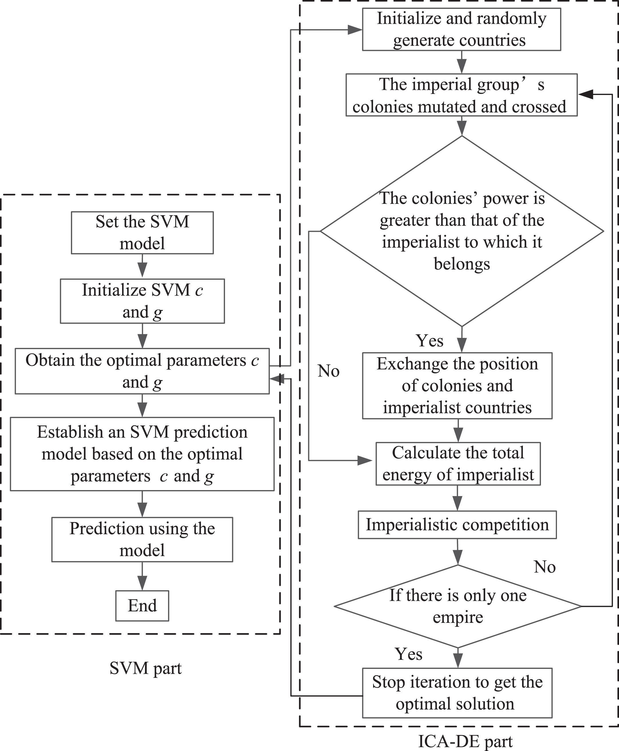
The framework of the ICA-DE-SVM model.

3.4 The framework of energy consumption prediction method for chillers based on ICA-DE-SVM

The flow chart of energy consumption prediction method for chillers based on ICA-DE-SVM is shown in Fig. 11. The steps are as follows:

Fig. 11

The flow chart of the proposed model for chillers.

Collect operation data set of multi chiller system: Y_i = { y_i1, y_i2, ⋯ , y_in } ∈ R^m×n. n is the number of variables, m is the number of samples;

Statistical analysis of collected data, as well as variable correlation analysis, to eliminate variables with high correlation. The eliminated variables are then fed into the network model via principal component analysis;

Input data into the ICA-DE-SVM model to predict energy consumption.

4 Experimental research

In the experiment, it is assumed that the chillers can work normally and that their performance is not affected by the increased operation time. Moreover, the failure rate of the chillers will not change with the extension of the operation time.

4.1 Collection of experimental data

The operation data set of the chiller is used to confirm the availability of the proposed model, The dataset used in this experiment is collected from the operational datasets of an actual chiller in a building in Panyu District, Guangzhou, China. The building’s area is 5372 m², and the total construction area is 111000 m². The ground area of the building is 48 floors, with 3 floors on the ground and a building height of 178 m. The central air-conditioning refrigeration station of the building mainly includes four chillers, four cooling water pumps, eight cooling towers, four chilled water pumps, and the total cooling capacity of the cold source system is rated at 8440 kW, as shown in Fig. 12. and Table 2. The building monitors and stores the operation data of the chiller in real time through the IBMS.

Fig. 12

Refrigeration station.

Table 2

The building type

Component	Features
Location	Panyu District, Guangzhou, China
Area	5372 m²
Construction area	111000 m²
Floor	48 floors above ground, 3 floors underground
Height	178 m
Total cooling capacity	8440 kW

Operational data was collected from July to August, 2022 using sensors that were installed. The variables for data collection include T_h1, T_h2, Q_ch, Q_cl, T_c1, T_c2, COP, W, PLR, T₀, T_hu, and T_wb. A total of 12000 sets of data were collected through the sensors that were installed. Part of the operational data collected is shown in Table 3. The sample data for T_h1, T_h2, T_c1, and T_c2 are shown in Fig. 8. Figure 13 shows that the working conditions of the central air conditioning cold source system parameters are always changing, and these four variables show periodic changes.

Table 3

Part of operation data

Number	Variables												Energy consumption (KW)
	PLR	W	COP	T _h2	Q _ch	T _h1	T _c1	Q _cl	T _c2	T ₀	T _hu	T _wb
	(%)	(KW)		(°C)	(m³/h)	(°C)	(°C)	(m³/h)	(°C)	(°C)	(% RH)	(°C)
1	90	2365.00	6.53	11.20	490.46	7.1	34	485.74	29	29.96	76.18	26.48	362.22
2	90	2391.00	6.53	11.30	489.64	7.1	34	487.10	29	30.00	79.03	26.96	366.03
3	90	2437.00	6.53	11.40	495.03	7.2	34	490.50	29	30.00	79.75	27.07	373.03
4	60	1129.00	6.79	11.5	269.32	7.9	33	288.11	29	30	77.83	26.78	169.13
5	100	2456.00	6.49	11.6	494.95	7.3	34	489.97	29	29.96	78.65	26.86	378.65
6	70	1357.00	6.78	11.6	269.59	7.3	33	307.44	29	30	80.03	27.11	200.03
7	100	2469.00	6.48	11.7	490.09	7.4	34	484.23	29	30	79.2	26.99	381.13
8	70	1378.00	6.84	11.7	260.28	7.1	33	330.79	29	29.86	78.93	26.81	201.40
9	100	2440.00	6.41	11.6	483.52	7.3	35	477.88	30	29.86	77.83	26.64	380.66
10	70	1304.00	6.86	11.6	247.45	7	33	322.91	30	29.86	78.38	26.73	190.38
. . .	. . .	. . .	. . .	. . .	. . .	. . .	. . .	. . .	. . .	. . .	. . .	. . .	. . .
11999	60	1429.00	6.35	10	376.69	6.7	33	353.09	29	31.09	76.97	27.66	140.22
12000	50	996.00	7.5	10	305.63	7.2	32	285.58	29	31.09	77.8	27.79	225.12

Fig. 13

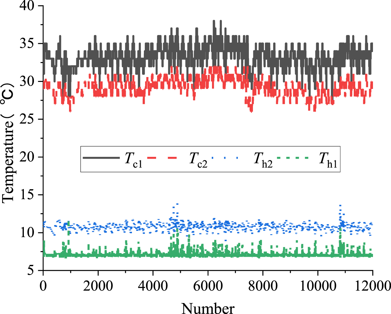
The sample data of some variables.

4.2 Correlation analysis

The violin diagram of 12000 sample datasets for each variable is shown in Fig. 14. The distribution of the variables in the sample data, including the maximum, minimum, median, and mean values of each variable, is shown in the box in the center of each violin diagram. The sample datasets for each variable are distributed within a particular range, and there are individual extreme values, as shown in Fig. 14. A normal distribution trend may be seen in the sample data distribution.

Fig. 14

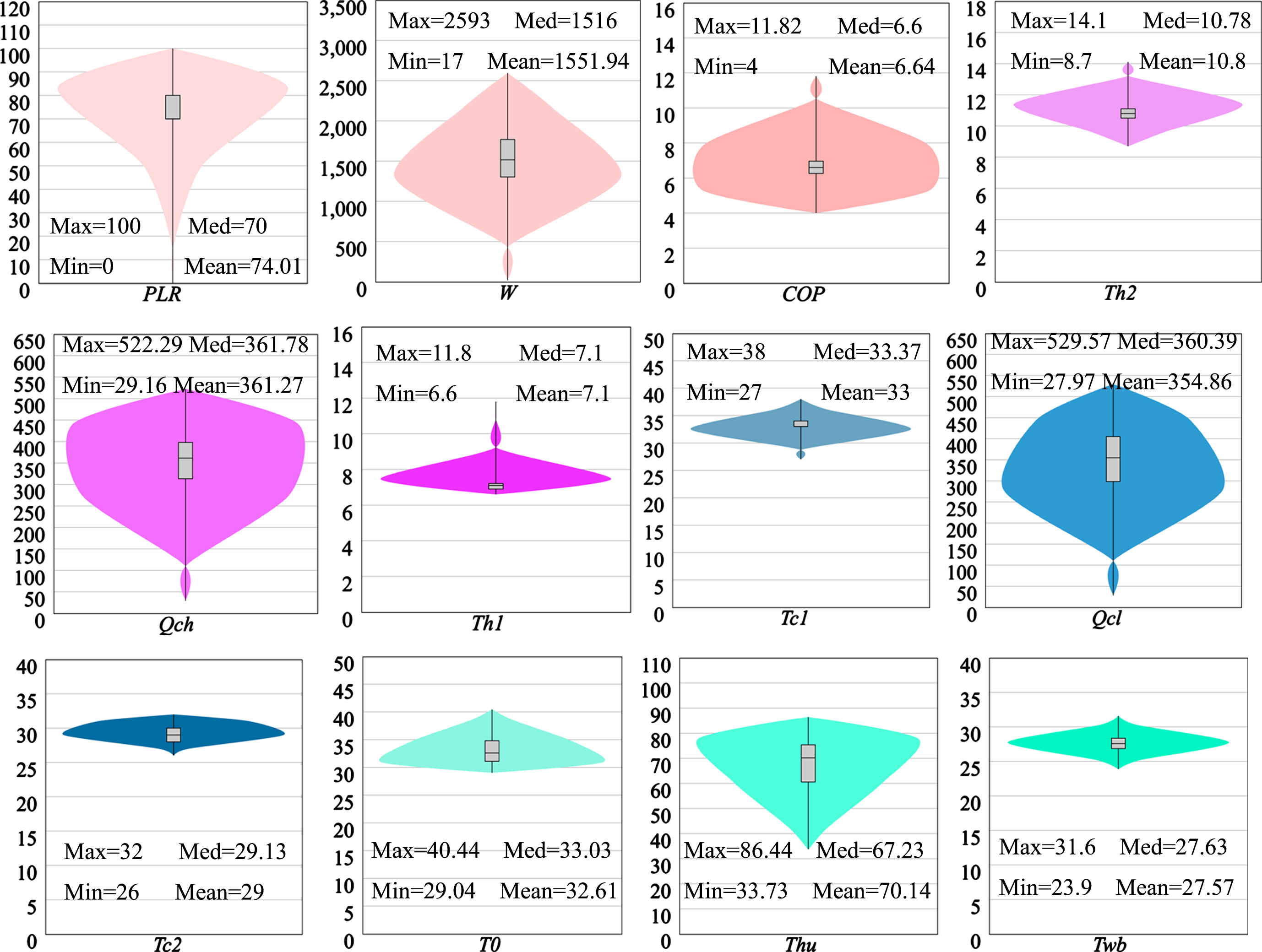
Violin chart of 12 variables.

In order to improve the accuracy of the established ICA-DE-SVM model, it is necessary to carry out correlation analysis among variables in order to eliminate variables with high correlation. If not, the accuracy of the resulting model may be compromised. Therefore, the correlation between each variable is evaluated using the Pearson correlation coefficient [38]. Figure 15 displays the heat map of the Pearson correlation coefficient between variables. Figure 10 shows that there is a strong association between the two variables, PLR and W. PLR and W are eliminated, and then the eliminated variables are input through principal component analysis processing into the network model.

Fig. 15

The correlation heat map.

4.3 Results

To evaluate the usefulness and adaptability of the established ICA-DE-SVM model, then conduct 9 experiments with different training sets. The training set is randomly generated. The number of training datasets was N, which was set to 2000, 2500, 3000, 3500, 4000, 4500, 5000, 5500, and 6000, respectively. Then the ICA-DE-SVM energy consumption prediction model was established. To evaluate the accuracy of the ICA-DE-SVM method, the absolute relative errors (ARE), mean absolute percentage error (MAPE), mean square error (MSE), and coefficient of determination (R²) were used as the evaluation criteria of the ICA-DE-SVM model. The smaller ARE and MAPE, the higher model accuracy. The closer R² is to 1, the higher model accuracy.

The equations are as follows: $ARE = | \frac{{\hat{y}}_{i} - y_{i}}{y_{i}} | \times 100 %$ (25) $MAPE = \frac{100 %}{n} \sum_{i = 1}^{n} | \frac{{\hat{y}}_{i} - y_{i}}{y_{i}} |$ (26) $MSE = \frac{1}{n} \sum_{i = 1}^{n} {({\hat{y}}_{i} - y_{i})}^{2}$ (27) $R^{2} = \frac{1}{n} \frac{\sum_{i = 1}^{n} {({\hat{y}}_{i} - {\bar{y}}_{i})}^{2}}{\sum_{i = 1}^{n} {({\bar{y}}_{i} - y_{i})}^{2}}$ (28) ${\bar{y}}_{i} = \frac{\sum_{i = 1}^{n} y_{i}}{n}$ (29) where n represents the quantity of samples, ${\hat{y}}_{i}$ is the predicted value of energy consumption, and y_i is the actual value of energy consumption. The MAPE, MSE, and R² of the ICA-DE-SVM energy consumption prediction model were established for 9 different training sets, as shown in Table 4.

Table 4

MAPE (%), MSE, and R² of the ICA-DE-SVM model

Number of training sets	MAPE	MSE	R ²
2000	0.91	8.4357	0.9844
2500	0.78	7.3000	0.9868
3000	0.70	6.2000	0.9981
3500	0.66	5.6574	0.9983
4000	0.55	5.5475	0.9984
4500	0.50	5.4469	0.9986
5000	0.47	2.9112	0.9993
5500	0.44	2.1700	0.9994
6000	0.42	1.6900	0.9995

Table 4 shows that when the training set number are 2000, the MAPE, MSE, and R² of the ICA-DE-SVM model are 0.91, 8.4357, and 0.9844, respectively; when the training set number are 2500, the MAPE, MSE, and R² of the ICA-DE-SVM model are 0.78, 7.3, and 0.9868, respectively; when the training set number are 3000, the MAPE, MSE, and R² of the ICA-DE-SVM model are 0.7, 6.2, and 0.9981, respectively; when the training set number are 3500, the MAPE, MSE, and R² of the ICA-DE-SVM model are 0.66, 5.6574, and 0.9983, respectively; when the training set number are 4000, the MAPE, MSE, and R² of the ICA-DE-SVM model are 0.55, 5.5475, and 0.9984, respectively; when the training set number are 4500, the MAPE, MSE, and R² of the ICA-DE-SVM model are 0.5, 5.4469, and 0.9986, respectively; when the training set number are 5000, the MAPE, MSE, and R² of the ICA-DE-SVM model are 0.47, 2.9112, and 0.9993, respectively; when the training set number are 5500, the MAPE, MSE, and R² of the ICA-DE-SVM model are 0.44, 2.17, and 0.9994, respectively; when the training set number are 6000, the MAPE, MSE, and R² of the ICA-DE-SVM model are 0.42, 1.69, and 0.9995, respectively. It is not difficult to see that as the quantity of training samples increases, the value of MAPE decreases, the value of MSE also decreases, and the value of R² is closer to 1. Due to the nonlinear, hysteretic, complex operating, time-varying, and strong coupling conditions of the cold source system, its actual energy consumption optimization is costly and time-consuming. The above experiments fully verify the effectiveness of the ICA-DE-SVM model, especially when the number of training datasets is large. It has obvious advantages. When dealing with the energy consumption prediction problem for chillers, the ICA-DE-SVM model could obtain good prediction results.

The ARE of the ICA-DE-SVM model for training sets, which was set to 2000, and testing sets, which was set to 500, are shown in Fig. 16. Most error using ARE of the ICA-DE-SVM model is less than 5%, which can satisfy the demand. Table 4 and Fig. 16 show that the established ICA-DE-SVM energy consumption prediction model for chillers meets the requirements, and the larger the number of training sets, the better the accuracy of the model.

Fig. 16

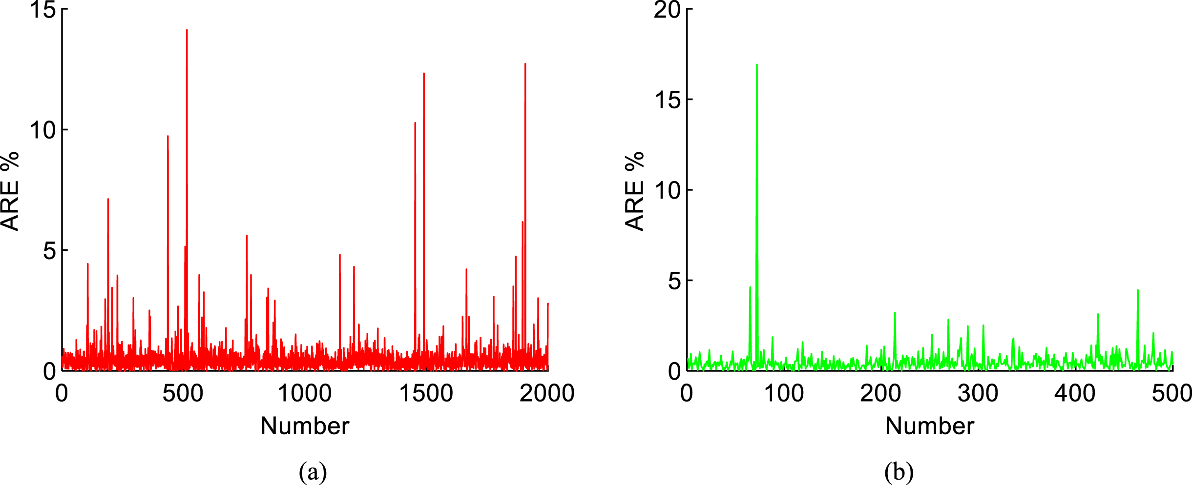
ARE of the proposed model: (a) using testing data, and (b) using training data.

To further verify the accuracy of the proposed model, the energy consumption values corresponding to 2000 sets of training datasets and 500 sets of testing datasets were calculated using the ICA-DE-SVM model and compared with the actual values. The results are shown in Fig. 17. Figure 17 shows that the predicted energy consumption value is relatively close to the actual value, which further illustrates the validity of the established model.

Fig. 17

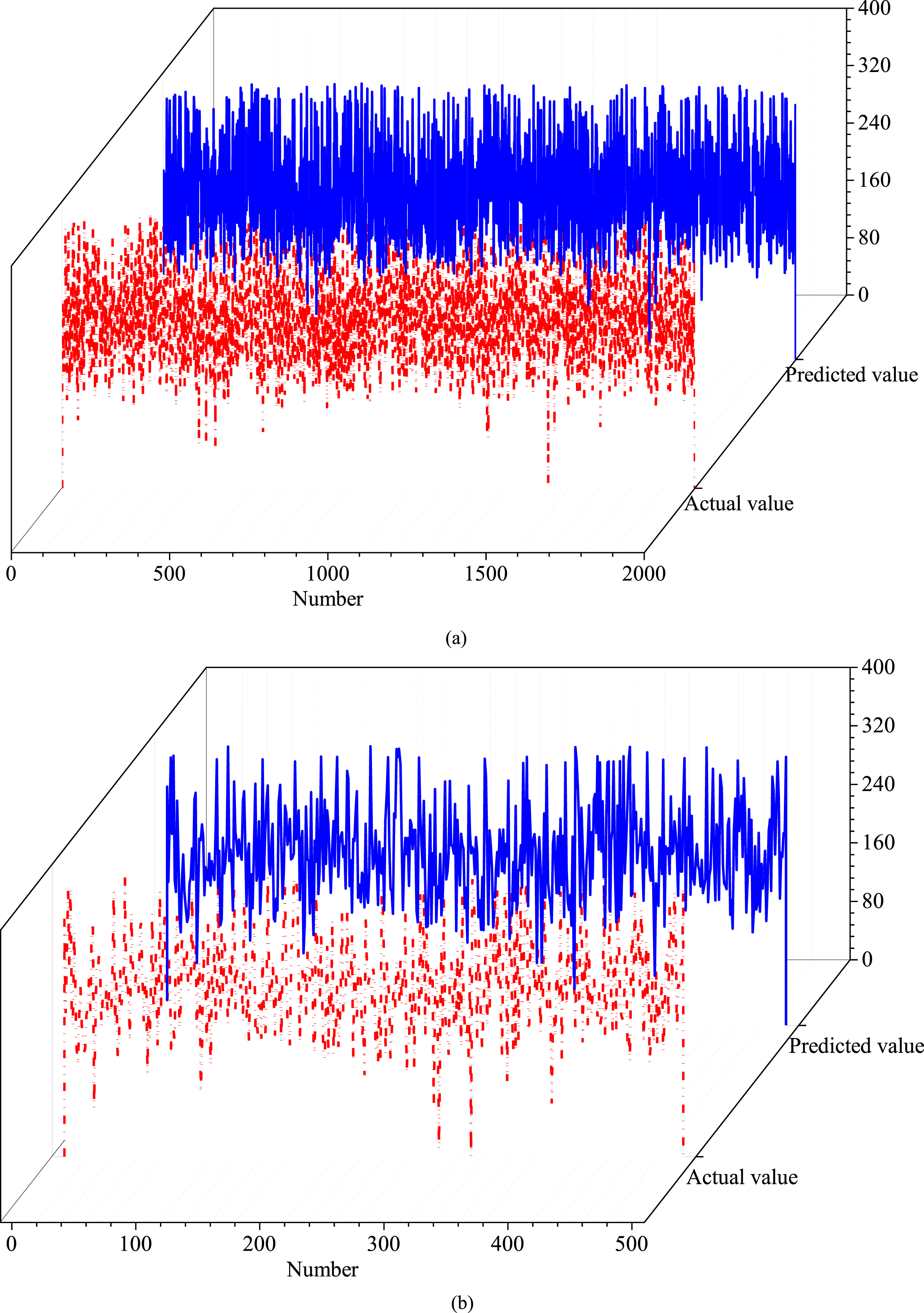
The actual value and predicted value of energy consumption: (a) using training data, (b) using testing data.

4.4 Comparative experiments

In this section, several sets of comparative experiments were designed. The SVM model, PSO-SVM model, GA-SVM model, WOA-SVM model, and ICA-SVM model were compared with the ICA-DE-SVM model, respectively. To facilitate a comprehensive comparison of the performance of each model, we conducted 10 experiments with training sets of the same number. The training set is randomly generated. In 10 trials, set the training set to 6000. The MAPE, MSE, and R² for each model can be calculated via Equations (26) –(29). The box plots of three evaluation indexes, MAPE, MSE, and R², are shown in Fig. 18.

Fig. 18

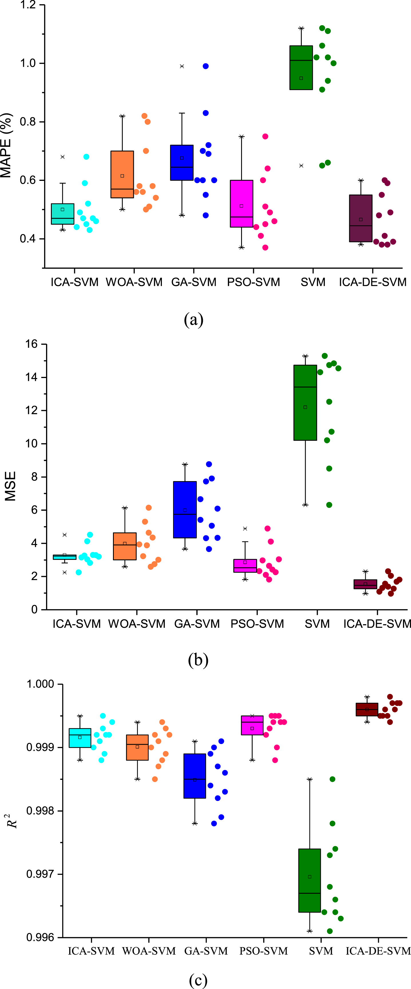
Box plot conducting 10 experiments: (a) box plot of MAPE, (b) box plot of MSE, (c) box plot of R².

Figure 18 depicts the maximum, minimum, and median values of the three performance indicators MAPE, MSE, and R² for the six energy prediction models. Figure 18 shows that the maximum and minimum MAPE values of the ICA-DE-SVM model are 0.60 and 0.38, respectively, the maximum and minimum MSE values are 2.3 and 0.9645, which are smaller than those of other models, and the maximum and minimum R² values are 0.9998 and 0.9994, which are larger than those of other models. This demonstrates that the ICA-DE-SVM model outperforms other models.

The MAPE, MSE, and R² values of the ICA-SVM model and the PSO-SVM model differ by only a small amount, indicating that they perform similarly when it comes to predicting energy consumption. The SVM model has the lowest accuracy. The GA-SVM model has higher precision than SVM but lower precision than other models.

5 Conclusions and prospects

In order to predict the energy consumption of the chiller, a method based on ICA-DE-SVM is proposed. To further improve the usefulness and adaptability of the proposed model, the Pearson correlation coefficient was used to analyze the correlation between each variable and then to eliminate variables with high correlation. Then the eliminated variables are input through principal component analysis processing into the network model.

The usefulness and adaptability of the ICA-DE-SVM model were verified on the actual cold source system. The results show that as the quantity of sample datasets increases, the value of MAPE decreases, the value of MSE also decreases, and the value of R² is closer to 1. However, the training time also increases. To select the optimal population numbers, it is necessary to consider both the training time and the values of the evaluation indices at the same time. And from Table 4, the optimal population numbers of the proposed model can be seen clearly is 5000 (MAPE = 0.47, MSE = 2.9112, R2 = 0.9993). This can be a good reference in an actual multi-chiller system in a building. Finally, the ICA-DE-SVM method was compared with the SVM model, PSO-SVM model, GA-SVM model, WOA-SVM model, and ICA-SVM model, respectively, and the results show a better performance of this proposed method.

In reality, as the amount of running time increases, the cold water host’s performance will suffer. With longer operating times, the failure rate of the chiller will rise. The model’s prediction error would progressively rise in the latter stage when it was trained on the earlier running data. Therefore, in future work, focus our attention on the following two aspects: (1) Due to the complexity and variability of the operating environment of the chiller, more input variables need to be considered. (2) The performance of the equipment needs to be considered.

Declaration of competing interest

The authors declare that they have no conflict of interest.

Acknowledgment

This research has received funding from the National Natural Science Foundation of China under Grant U1501248 and Grant 51905109, the Foshan Key Field Project of Science and Technology under Grant No. 2020001006509.

References

Wang

, Guo

, Chen

, et al., Carbon peak and carbon neutrality in China: G oals, implementation path and prospects, China Geology 4(4) (2021), 720–746.

Lam

J.C.

, Wan

K.K.

, Tsang

and Yang

, Building energy efficiency in different climates, Energy Convers Manage 49(8) (2008), 2354–2366.

Peng

, Rysanek

, Nagy

and Schlüter

, Using machine learning techniques for occupancy-prediction-based cooling control in office buildings [J], Appl Energy 211 (2018), 1343–1358.

Afram

and Janabi-Sharifi

, Review of modeling methods for HVAC systems, Appl Therm Eng 67(1-2) (2014), 507–519.

Kassas

, Modeling and simulation of residential HVAC systems energy consumption, Procedia Comput Sci 52 (2015), 754–763.

Afram

and Janabi-Sharifi

, Gray-box modeling and validation of residential HVAC system for control system design, Appl Energy 137 (2015), 134–150.

Afram

and Janabi-Sharifi

, Black-box modeling of residential HVAC system and comparison of gray-box and black-box modeling methods, Energy Build 94 (2015), 121–149.

Massana

, Pous

, Burgas

, Melendez

and Colomer

, Short-term load forecasting in a non-residential building contrasting models and attributes, Energy Build 92 (2015), 322–330.

Lim

H.S.

and Kim

, Prediction model of Cooling Load considering time-lag for preemptive action in buildings, Energy Build 151 (2017), 53–65.

10.

Braun

, Altan

and Beck

, Using regression analysis to predict the future energy consumption of a supermarket in the UK, Appl Energy 130 (2014), 305–313.

11.

Chou

J-S.

and Ngo

N-T.

, Time series analytics using sliding window metaheuristic optimization-based machine learning system for identifying building energy consumption patterns, Appl Energy 177 (2016), 751–770.

12.

Zeng

, Liu

and Yu

, Comparative study of data driven methods in building electricity use prediction [J], Energy Build 194 (2019), 289–300.

13.

Kim

J-H.

, Seong

N-C.

and Choi

, Modeling and optimizing a chiller system using a machine learning algorithm, Energies 12(15) (2019), 2860.

14.

, Xiao

, Zhang

and Fan

, Attention-based interpretable neural network for building cooling load prediction, Appl Energy 299 (2021), 117238.

15.

Wang

, Lu

and Feng

, A novel improved model for building energy consumption prediction based on model integration, Appl Energy 262 (2020), 114561.

16.

, Li

, Garg

, et al., An adaptive boosting charging strategy optimization based on thermoelectric-aging model, surrogates and multi-objective optimization, Applied Energy 312 (2022), 118795.

17.

, Li

, Mou

, et al., A Hybrid Battery Equivalent Circuit Model, Deep learning, and Transfer Learning for Battery State Monitoring, IEEE Transactions on Transportation Electrification, 2022.

18.

Guidotti

, Monreale

, Ruggieri

, Turini

, Giannotti

and Pedreschi

, A survey of methods for explaining black box models, ACM Comput Surv 51(5) (2018), 1–42.

19.

Zhao

and Liu

, A hybrid method of dynamic cooling and heating load forecasting for office buildings based on artificial intelligence and regression analysis [J], Energy Build 174 (2018), 293–308.

20.

Tang

, Kusiak

and Wei

, Modeling and short-term prediction of HVAC system with a clustering algorithm, Energy Build 82 (2014), 310–321.

21.

Paudel

, Elmitri

, Couturier

, et al., A relevant data selection method for energy consumption prediction of low energy building based on support vector machine, Energy and Buildings 138 (2017), 240–256.

22.

Jing

, Yu

, Luo

, et al., Energy-saving diagnosis model of central air-conditioning refrigeration system in large shopping mall, Energy Reports 7 (2021), 4035–4046.

23.

Ding

, Zhang

and Yuan

, Research on short-term and ultra-short-term cooling load prediction models for office buildings, Energy and Buildings 154 (2017), 254–267.

24.

Atashpaz-Gargari

and Lucas

, Imperialist competitive algorithm: an algorithm for optimization inspired by imperialistic competition[C]//2007 IEEE congress on evolutionary computation, IEEE (2007), 4661–4667.

25.

Moradi

, Abdi

, Lumbreras

, et al., Transmission Expansion Planning in the presence of wind farms with a mixed AC and DC power flow model using an Imperialist Competitive Algorithm, Electric Power Systems Research 140 (2016), 493–506.

26.

Khosravi

, Banejad

and Shandiz

H.T.

, Robust dynamic state estimation of power system using imperialist competitive algorithm, Canadian Journal of Electrical and Computer Engineering 41(2) (2018), 64–76.

27.

Gerist

and Maheri

M.R.

, Structural damage detection using imperialist competitive algorithm and damage function, Applied Soft Computing 77 (2019), 1–23.

28.

Mollajan

, Memarian

and Quintal

, Nonlinear rock-physics inversion using artificial neural network optimized by imperialist competitive algorithm, Journal of Applied Geophysics 155 (2018), 138–148.

29.

Hmida

J.B.

, Chambers

and Lee

, Solving constrained optimal power flow with renewables using hybrid modified imperialist competitive algorithm and sequential quadratic programming, Electr Power Syst Res 177 (2019), 105989.

30.

Aliniya

and Mirroshandel

S.A.

, A novel combinatorial merge-split approach for automatic clustering using imperialist competitive algorithm, Expert Syst Appl 117 (2019), 243–266.

31.

Gerist

and Maheri

M.R.

, Structural damage detection using imperialist competitive algorithm and damage function, Appl Soft Comput 77 (2019), 1–23.

32.

Aghdam

F.H.

and Hagh

M.T.

, Security constrained unit commitment (SCUC) formulation and its solving with modified imperialist competitive algorithm (MICA), J King Saud Univ-Eng Sc 2017.

33.

Rabiee

, Sadeghi

and Aghaei

, Modified imperialist competitive algorithm for environmental constrained energy management of microgrids, J Clean Product 202 (2018), 273–292.

34.

, Yang

, Pan

, et al., A novel deep stacking least squares support vector machine for rolling bearing fault diagnosis, Computer Ind 110 (2019), 36–47.

35.

Song

, Lei

, Chen

, et al., Multiple facial image features-based recognition for the automatic diagnosis of turner syndrome, Computer Ind 100 (2018), 85–95.

36.

Dias

A.L.

, Turcato

A.C.

, Sestito

G.S.

, et al., A cloud-based condition monitoring system for fault detection in rotating machines using PROFINET process data, Computer Ind 126 (2021), 103394.

37.

Han

Y.B.

, Bai

G.C.

, Li

X.Y.

, et al., Dynamic reliability analysis of flexible mechanism based on support vector machine, Journal of Mechanical Engineering 50(11) (2014), 86–92.

38.

Chen

, Deng

, Ren

, et al., A new energy consumption prediction method for chillers based on GraphSAGE by combining empirical knowledge and operating data, Applied Energy 310 (2022), 118410.