ITARA and ELECTRE III three-way decision model in the spherical fuzzy environment and its application in customer selection

Abstract

As COVID-19 swept through, production in various industries was affected. Epidemic control leads to logistical disruptions from time to time and suppliers have to make production and shipping decisions after analyzing the customer’s situation. Therefore, the majority of manufacturers need to establish effective methods for the selection of distribution customers. The method presented in this paper can classify customers into three regions and rank their status to help suppliers effectively make decisions. The three-way decision (3WD) is a well-known fast sorting method in multi-attribute decision-making (MADM). In this paper, we proposed the 3WD model based on Indifference Threshold based Attribute Ratio Analysis (ITARA), ELimination Et Choix Traduisant la REalite III (ELLECTRE III) in the spherical fuzzy environment. Then, we used the SF-ITARA-ELECTRE III-3WD method to select the suitable customers for dispensing. In addition, comparison with the conventional SF-PROMETHEE-3WD, SF-EVAMIX-3WD, SF-TOPSIS-3WD and SF-VIKOR-3WD are created to verify the effectiveness of the proposed method. An effective risk-averse solution to the MADM problem for spherical fuzzy environment is provided.

Keywords

3WD ITARA ELECTRE III spherical fuzzy number (SFN)customers selection

1 Introduction

With the development of decision science, the multi-attribute decision-making (MADM) method has become more and more relevant to practical decision-making and has been applied in more and more fields. Three-way decision (3WD) [1] breaks the traditional "yes" or "no" model of decision-making and introduces the option of delayed decision-making, which is more in line with the actual situation where experts cannot give a definite answer when information is incomplete. Indifference Threshold based Attribute Ratio Analysis (ITARA) [2] is an attribute weight determination method proposed by Mohammad in 2019, which uses the gap in decision information between the same attribute to determine the weight adjustment coefficients, which in turn results in attribute weights. It is a combination of subjective and objective empowerment method because it applies to artificially specified undifferentiated thresholds. ELimination Et Choix Traduisant la REalite III (ELECTRE III) [3] is a MADM method based on the idea of pairwise comparison proposed by Roy, which uses the dominant relationship between schemes for decision-making. The improved ELECTRE III approach outperforms the original ELECTRE III method in terms of identifying the positive and negative aspects of relationships between evaluation data in a fuzzy environment. With good results, traditional ELECTRE III has been applied to a specific set of choice issues, but as these problems become more complicated, more and more of them are being extended to the fuzzy environment. ELECTRE III circumvents the drawbacks of transforming fuzzy numbers into exact numbers, which can alter the decision results, by employing the distance measure between fuzzy numbers to assess the superiority and inferiority of each solution. It has been applied to a variety of fuzzy environments because of the reliability of the results obtained. Spherical fuzzy sets (SFS) [4] is extended by picture fuzzy sets (PFS), which also contain four parameters: membership, neutral membership, non-membership and rejection, but its parameter space is broader than PFS, so it is widely used in MADM problems. In this paper, we proposed the 3WD model for ITARA and ELECTRE III in the spherical fuzzy environment. The contributions are as follows:

ITARA is a practical method of determining weights that combines subjective and objective aspects and can take into account both expert opinions and the characteristics of the decision information itself. The spherical fuzzy environment is also widely used in today’s decision-making environment. We extended the application of ITARA to the spherical fuzzy environment can provide a more practical method for determining attribute weights.

The ELECTRE III method is improved by not using the traditional defuzzification operation, but by using the distance between each decision information and the positive ideal decision information to determine the dominance relationship between them. The results obtained are not affected by the error of the defuzzification operation, and the results obtained are more accurate, ensuring that ELECTRE III functions well.

We proposed the improved 3WD method in the spherical fuzzy environment, whose loss function is derived from the distance between evaluation information (spherical fuzzy numbers (SFNs)), the properties of the evaluation information itself can be well used, and the risk assessment parameters σ are added, which can effectively control the risk in the decision making process.

Based on the special scenario of COVID-19, it breaks away from the traditional customer selection perspective and focuses on the rational allocation of resources based on the customer’s situation when resources are limited and logistics are obstructed. The methodology proposed in this paper can effectively solve this problem.

In the existing literature, most suppliers are chosen from the perspective of the customer, and when confronted with an unexpected situation, there is a shortage of supplier resources. In this case, the supplier’s indifferent treatment of the customer may result in resource waste. If the customer’s urgency and accessibility can be classified and ranked prior to taking supply measures, the customer can receive the required goods as soon as possible with the least amount of resource waste. The method proposed in this paper can significantly improve resource allocation efficiency in an environment where resources are limited and logistics are hampered in some areas.

The paper is structured as follows: the 2nd section is about the research of SFS, ITARA, ELECTRE III, and 3WD. The 3rd section introduces the classical SFS, ITARA, ELECTRE III, and 3WD contents. The 4th section proposes the SF-ITARA-ELECTRE III-3WD model. In the 5th section, the proposed method is used to analyze the customer selection problem in the COVID-19 spreading environment. The results are compared with the classical method, and sensitivity analysis is also performed in this section. Finally, a summary of the proposed method is presented in the 6th section.

2 Literature review

Realistic decision scenarios are full of uncertainty and fuzziness, and the description of decision information by exact numbers cannot fully show the real situation. To more accurately describe decision information, Zadeh proposed the concept of fuzzy sets (FS) in 1965 [5], which expresses the possibility of event occurrence in terms of membership. Atanassov added the non-membership degree to it and FS is extended to intuitionistic fuzzy sets (IFS) [6]. Due to the rule that the sum of membership and non-membership must be less than or equal to 1, some events cannot be described exhaustively. Yager extended the IFS to Pythagorean fuzzy sets (PyFS) [7] and specifics that the sum of squares of membership and non-membership is less than 1. To be more relevant to real-life scenarios, Cuong expanded IFS to PFS [8], and he added neutral membership to describe the event situation. Because it fits the actual decision-making scenario, it has been successfully applied in recent years in service satisfaction survey, third-party logistics service provider selection, etc [9 –12]. To extend the parameter spaces of membership, neutral-membership, non-membership, and rejection, Mahmood extended PFS to SFS and T-spherical fuzzy sets (T-SFS), adds another tool to the description of decision information. And it has been widely used in investment selection problem [13], photovoltaic cells selection [14], and product reviews [15] fields, etc.

EWM was originally proposed by Shannon and Weaver in 1947. Entropy is originally a concept in physics to indicate the degree of chaos, and was later extended to information theory. The smaller the entropy of information in a system, the more discrete the information is and the less information is provided, and conversely, the greater the entropy of information, the less discrete the information is within its system and the more information is provided. Therefore, EWM solves the attribute weights based on the magnitude of the coefficient of variation of the indicators, which is an objective weighting method. Level based weight assessment (LBWA) [16] is an attribute weight determination method proposed by Zizovic and Pamucar, in which the most important attribute is first specified by experts, then the importance of the attribute is ranked based on experience, and finally the combined attribute weights are obtained by combining the results of all experts’ attribute weight determinations. The Full Consistency Method (FUCOM) [17] is an a priori ranking-based attribute weight determination method proposed by Pamucar, in which the decision maker first ranks the importance of the attributes then determines the relative number of importance among them, and finally determines the attribute weights. ITARA is a combined subjective and objective attribute weight determination method proposed by Mohammad, which is based on the principle of comparing the gap between decision information with the acceptable non-differentiation threshold under the same attribute, and then obtaining the attribute weight adjustment values, the attribute weights. The advantage of this method is that it makes good use of the decision information itself while taking into account the actual situation and expert preferences, and results in more objective attribute weights. Due to its flexibility, it has been widely used in recent years. Sofuoglu [18] used the ITARA method in material selection analysis to compensate for the inadequacy of subjective evaluation attributes and constructed the ITARA-TOPSIS, ITARA-MOORA, and ITARA-VIKOR models for the selection of the selected materials, the results were successful. Ulutaş et al. [19] used the correlation coefficient and the standard deviation (CCSD method) in combination with the ITARA method to determine the weights of the attributes to select the evaluation of logistics equipment, and the results of the weights obtained were highly reliable, combined with the compromise solution method (MARCOS) method for the selection of manual stacker cranes for small warehouses. Liu et al. [20] used ITARA to calculate the attribute weights in the selection problem of a department manager of an investment company and created the q-RONFNs-ITARA-MABAC method to evaluate the selection of several candidates, obtained reliable and robust results. In this paper, ITARA is chosen as the attribute weight determination method because the complexity of the decision environment requires mediation of the acceptable degree of differences between attributes.

The ELECTRE [21] was used by Roy in 1965 for the Paris Metro project, formalizing the methodology in 1985, and its principle is to construct a weak sequential relationship to determine the ranking of schemes. Due to its good results, it has been continuously developed and applied. It was expanded to the ELECTRE II method, which obtained the ranking of schemes by evaluating the strong and weak relationships between schemes. These method has been widely used since its emergence, Yadav et al. [22] used the BWM-ELECTRE model to assess the sustainability of the supply chain and derive a reference solution for supply chain management in the context of Industry 4.0. Zhou et al. [23] used the Fermatean fuzzy-ELECTRE model in their notational analysis of the site selection problem for the construction of the Wuhan Square Cabin Hospital, which provided effective suggestions for site selection. Liu et al. [24] used the TODIM-ELECTRE II method in linguistic Z-number sets to compare the advantageous relationships among technologies in an example of end-of-pipe wastewater curing technology selection. ELECTRE III is an efficient ranking method, which represents the superiority relationship between two schemes as a binary relationship by giving undifferentiated thresholds, preference thresholds, and denial thresholds. It only cares about the dominant relationship between schemes rather than the exact number, which largely eliminates the influence of uncertain and fuzzy evaluation information on the ranking. Due to its good effect, it has been applied in many fields. Chen et al. [25] used the hesitant fuzzy linguistic term sets ELECTRE III model to analyze its advantages in the contractor selection case, which better handles the uncertainty and fuzziness of the linguistic term set and yields scientific results. Peng et al. [26] constructed a Z-number-regret theory-ELECTRE III model for measuring the risk problem of new energy investment, and discussed the results using the new energy investment in the Qingshui Tang Industrial Zone as an example, concluded that solar energy is the best option. ELECTRE III has been applied to a variety of fuzzy environments and has addressed issues such as the haze management issues [27], water resources human recharge station selection [28], and the construction contractor selection [29] etc.

In 1982, Pawlak proposed rough set (RS) [30] theory to process data intelligently. Based on decision-theoretic rough sets (DTRS), Yao proposed 3WD theory in 2009, which is divided schemes into three regions, positive region, boundary region, and negative region. According to Bayesian minimal decision theory, 3WD determines the divisions and ranking of the schemes by comparing the expected loss, which is derived from two important parameters possibility and loss function. In recent years, 3WD has also been improved and applied by scholars. Miao et al. [31] extended 3WD to PyFS and used the idea of 3WD to measure MADM problems to demonstrate the classification of solutions using the same set of thresholds. Xu [32] proposed a 3WD model based on double hierarchy Hamacher operators, which effectively solved the problem of selection of cooperative enterprises during the period of COVID-19. Wang et al. [33] argued that 3WD provides a new perspective to solve the uncertain MADM problem and helps in risk aversion. Therefore, they extended 3WD to interval type-2 fuzzy environment and introduced regret theory to solve the decision problem. Wu et al. in their study of 3WD loss function thresholds found that the thresholds are not related to the loss values themselves, to the difference between their loss values, so the determination of the loss function was improved.

For the current research we found that the spherical fuzzy environment can provide a more flexible decision environment for decision makers yet no subjective parameters have been introduced in the attribute determination, and the application of ELECTRE III in the spherical fuzzy environment is still stuck in simple defuzzification after calculation. More importantly, spherical fuzzy MADM requires a faster alternative classification method, and the improved 3WD happens to be a widely used method but never used in spherical fuzzy environments.

3 Preliminary knowledges

In this section, we introduce the basics of SFS, ITARA, ELECTRE III, and 3WD.

3.1 Spherical fuzzy sets and spherical fuzzy numbers

Definition 1. For any universal set X, an IFS is defined as $A = {< X, μ (x), η (x) > | x \in X}$ (1)

where μ_A (x) : X → [0, 1] , η_A (x) : X → [0, 1] represent the degree of membership and non-membership, respectively, which satisfy the condition 0 ≤ μ_A (x) + η_A (x) ≤1. When η_A (x) =0 it degenerates into fuzzy sets (FS). The hesitation is v_A (x) =1 - μ_A (x) - η_A (x). For simplification, we denote the A =< μ_A, η_A > as intuitionistic fuzzy number (IFN).

Definition 2. For any universal set X, an PyFS is defined as $A = {< X, μ (x), η (x) > | x \in X}$ (2)

where μ_A (x) : X → [0, 1] , η_A (x) : X → [0, 1] represent the degree of membership and non-membership, respectively, which satisfy the condition $0 \leq \underset{A}{μ^{2}} (x) + \underset{A}{η^{2}} (x) \leq 1$ . The hesitation is $v_{A} (x) = \sqrt{1 - \underset{A}{μ^{2}} (x) - \underset{A}{η^{2}} (x)}$ . For simplification, we denote the A =< μ_A, η_A > as Pythagorean fuzzy number (PyFN).

Definition 3. For any universal set X, an PFS is defined as $A = {< X, μ (x), η (x), ν (x) > | x \in X}$ (3)

where μ_A (x) : X → [0, 1] , η_A (x) : X → [0, 1] and ν_A (x) : X → [0, 1] represent the degree of membership, neutral membership, and non-membership, respectively, which satisfy the condition 0 ≤ μ_A (x) + η_A (x) + ν_A (x) ≤1. When η_A (x) = ν_A (x) =0 it degenerates into FS. When η_A (x) =0 it degenerates into IFS. The refusal membership is π_A (x) =1 - μ_A (x) - η_A (x) - ν_A (x). For simplification, we denote the A =< μ_A, η_A, ν_A > as picture fuzzy number (PFN).

Definition 4. For any universal set X, an SFS is defined as $A = {< X, μ (x), η (x), ν (x) > | x \in X}$ (4)

where μ_A (x) : X → [0, 1] , η_A (x) : X → [0, 1] and ν_A (x) : X → [0, 1] represent the degree of membership, neutral membership, and non-membership, respectively, which satisfy the condition $0 \leq \underset{A}{μ^{2}} (x) + \underset{A}{η^{2}} (x) + \underset{A}{ν^{2}} (x) \leq 1$ . The refusal membership is $π_{A} (x) = \sqrt{1 - \underset{A}{μ^{2}} (x) - \underset{A}{η^{2}} (x) - \underset{A}{ν^{2}} (x)}$ . For simplification, we denote the A =< μ_A, η_A, ν_A > as SFN.

Definition 5. Let A =< μ_A, η_A, ν_A >, A₁ =< μ_{A
₁}, η_{A
₁}, ν_{A
₁} > and A₂ =< μ_{A
₂}, η_{A
₂}, ν_{A
₂} > be any three SFNs, and λ ≻ 0, the algorithm are as follows: $\begin{matrix} A_{1} \oplus A_{2} = < {(\underset{A_{1}}{μ^{2}} + \underset{A_{2}}{μ^{2}} - \underset{A_{1}}{μ^{2}} \underset{A_{2}}{μ^{2}})}^{1 / 2}, η_{A_{1}} η_{A_{2}}, \\ {((1 - \underset{A_{2}}{μ^{2}}) \underset{A_{1}}{ν^{2}} + (1 - \underset{A_{1}}{μ^{2}}) \underset{A_{2}}{ν^{2}} - \underset{A_{1}}{ν^{2}} \underset{A_{2}}{ν^{2}})}^{1 / 2} > \end{matrix}$ (5) $\begin{matrix} A_{1} \otimes A_{2} = < μ_{A_{1}} μ_{A_{2}}, {(\underset{A_{1}}{η^{2}} + \underset{A_{2}}{η^{2}} - \underset{A_{1}}{η^{2}} \underset{A_{2}}{η^{2}})}^{1 / 2}, \\ {((1 - \underset{A_{2}}{η^{2}}) \underset{A_{1}}{ν^{2}} + (1 - \underset{A_{1}}{η^{2}}) \underset{A_{2}}{ν^{2}} - \underset{A_{1}}{ν^{2}} \underset{A_{2}}{ν^{2}})}^{1 / 2} > \end{matrix}$ (6) $\begin{matrix} λ \cdot A = < {(1 - {(1 - \underset{A}{μ^{2}})}^{λ})}^{1 / 2}, \underset{A}{η^{λ}}, \\ {({(1 - \underset{A}{μ^{2}})}^{λ} - {(1 - \underset{A}{μ^{2}} - \underset{A}{ν^{2}})}^{λ})}^{1 / 2} > \end{matrix}$ (7) $\begin{matrix} A^{λ} = < \underset{A}{μ^{λ}}, {(1 - {(1 - \underset{A}{η^{2}})}^{λ})}^{1 / 2}, \\ {({(1 - \underset{A}{η^{2}})}^{λ} - {(1 - \underset{A}{η^{2}} - \underset{A}{ν^{2}})}^{λ})}^{1 / 2} > \end{matrix}$ (8)

Definition 6. Let A =< μ_A, η_A, ν_A >, the score function and accuracy function are as follows: $S (A) = {(2 μ_{A} - \frac{ν_{A}}{2})}^{2} - {(η_{A} - \frac{ν_{A}}{2})}^{2}$ (9) $Ac (A) = μ_{A}^{2} + η_{A}^{2} + ν_{A}^{2}$ (10)

Definition 7. For any two SFNs A₁ =< μ_{A
₁}, η_{A
₁}, ν_{A
₁} > and A₂ =< μ_{A
₂}, η_{A
₂}, ν_{A
₂} >.

(1) If S (A₁) ≻ S (A₂), then A₁ ≻ A₂,

(2) If S (A₁) = S (A₂), then

if Ac (A₁) ≻ Ac (A₂), then A₁ ≻ A₂,

if Ac (A₁) ≺ Ac (A₂), then A₁ ≺ A₂.

Definition 8. For two SFNs A₁ and A₂ defined above in x = {x₁, x₂, . . . , x_n}, the normalized Hamming distance is described as follows: $\begin{matrix} D_{H} = \frac{1}{n} \sum_{i = 1}^{n} (| \underset{A_{1}}{μ^{2}} (x_{i}) - \underset{A_{2}}{μ^{2}} (x_{i}) | + \\ | \underset{A_{1}}{η^{2}} (x_{i}) - \underset{A_{2}}{η^{2}} (x_{i}) | + | \underset{A_{1}}{ν^{2}} (x_{i}) - \underset{A_{2}}{ν^{2}} (x_{i}) |) \end{matrix}$ (11)

3.2 ITARA

Mohammad proposed a method for attribute weight determination by a combination of data itself and Indifferent threshold (IT_j). IT_j is generally given by experts. Its meaning is the level of variation between schemes under attribute j. Within the given value, it is considered as no variation between schemes. Proceed as follow:

Step 1. Construct the decision matrix that includes m schemes and n attributes, and determine its IT_j. a_ij represents the jth attribute of the ith scheme, and IT_j represents the IT of the jth attribute.

Step 2. Normalize the data and get the normalized indifference threshold (NIT_j). ${α_{i}}_{j} = \frac{a_{ij}}{\sum_{i = 1}^{m} a_{ij}}, \forall i \in m, j \in n$ (12) $NI T_{j} = \frac{I T_{j}}{\sum_{i = 1}^{m} a_{ij}}, \forall j \in n$ (13)

Step 3. Sort α_i_j in ascending order, mark as β_i_j.

Step 4. Calculate the difference between two adjacent values and get difference matrix γ_ij. $γ_{ij} = β_{i + 1, j} - β_{ij}$ (14)

Step 5. Compare γ_ij and NIT_j to determine the weight adjustment factor τ_j. ${τ_{i}}_{j} = {\begin{matrix} γ_{ij} - NI T_{j}, γ_{ij} ≻ NI T_{j} \\ 0, γ_{ij} \leq NI T_{j} \end{matrix}, \forall i \in m, j \in n$ (15)

If the difference between two adjacent decision information (γ_ij) is greater than the NIT_j, it has an impact on the attribute weight determination and should be attributed to the attribute weight adjustment factor τ_j.

Step 6. Calculate the total weight adjustment factor ν_ij with weight w_j. $ν_{ij} = \sum_{i = 1}^{m} τ_{ij}, w_{j} = \frac{ν_{ij}}{\sum_{j = 1}^{n} ν_{ij}}$ (16)

3.3 ELECTRE III

ELECTRE III is a MADM method in the European School, which inherits the European School’s idea [34] of hierarchical relationships in the decision-making process. It is based on the comparison of the schemes under each attribute to determine the dominant relationship and ultimately the scheme ranking.

The solution process consists of four parts, which are determining the threshold value (strictly better than the threshold p_j, non-differential threshold q_j, and veto threshold v_j), calculating the consistency index (C (i, k)), calculating the non-consistency index (d_j (i, k)), and calculating the credibility (S (i, k)) and ranking.

Firstly, assume that there are m schemes and n attributes with attribute weights w_j. a_ij denotes the evaluation value of the ith scheme under the jth attribute.

Step 1. Calculate the threshold values p_j, q_j and v_j.

The threshold is usually given by an experienced expert and satisfies the relation q_j ≤ p_j ≤ v_j.

It can also be obtained computationally. Corazza et al. [35] proposed the relation for determining the threshold from the extreme difference (S_j). $S_{j} = max a_{j} - min a_{j}, q_{j} = \frac{1}{6} S_{j}, p_{j} = \frac{2}{3} S_{j}, v_{j} = \frac{5}{6} S_{j}$ (17)

Step 2. Calculate consistency index (C (i, k)).

We define C (i, k) as the degree of dominance of scheme i over scheme k. For the degree of dominance under a single attribute weight we define c_j (i, k). Thus $C (i, k) = \frac{\sum_{j = 1}^{n} w_{j} c_{j} (i, k)}{\sum_{j = 1}^{n} w_{j}}$ (18) where $c_{j} (i, k) = {\begin{matrix} 0, {a_{k}}_{j} - a_{ij} \geq p_{j} \\ 1, {a_{k}}_{j} - a_{ij} \leq q_{j} \\ \frac{a_{ij} - a_{kj} + p_{j}}{p_{j} - q_{j}}, otherwise \end{matrix}$ (19)

For schemes i and k, the larger the difference, the smaller c_j (i, k). When c_j (i, k) =0, it indicates that scheme i is superior to k to the extent of 0 under attribute j and scheme k is strictly superior to scheme i. When c_j (i, k) =1, it indicates that there is no significant difference between scheme i and scheme k under attribute j.

Step 3. Calculate the non-conformity index (d_j (i, k)).

In contrast to consistency, non-consistency measures the degree to which scheme i is inferior to scheme k. $d_{j} (i, k) = {\begin{matrix} 0, {a_{k}}_{j} - a_{ij} \leq p_{j} \\ 1, {a_{k}}_{j} - a_{ij} \geq v_{j} \\ \frac{a_{kj} - a_{ij} - p_{j}}{v_{j} - p_{j}}, otherwise \end{matrix}$ (20)

For schemes i and k, the larger the difference, the larger d_j (i, k). When d_j (i, k) =0, indicates that the rejection of scheme i is better than the rejection of scheme k to the extent of 0, scheme i is not better than scheme k. When d_j (i, k) =1, indicating that rejection of scheme i is better than a rejection of scheme k to the extent of 1, scheme i is inferior to scheme k.

Step 4. Calculate credibility index (S (i, k)). $\begin{matrix} S (i, k) = \\ {\begin{matrix} C (i, k) \prod \frac{1 - d_{j} (i, k)}{1 - C (i, k)}, j \in n, d_{j} (i, k) ≻ C (i, k) \\ C (i, k), max {d_{j} (i, k)} \leq C (i, k) \end{matrix} \end{matrix}$ (21)

From S (i, k) we can see that the role of d_j (i, k) is mainly to make the poor data uncompensable. When scheme i is compared with scheme k, if d_j (i, k) =0, then S (i, k) =0 and the confidence that scheme i is better than scheme k is 0. We can get that even though most of the indicators are better than other schemes, a defect directly negates the scheme’s advantage. The d_j (i, k) makes decision more cautious.

Finally, we derive the net credibility and the ranking of the programs.

Calculate consistent confidence ( $B_{i}^{+}$ ) $\underset{i}{B^{+}} = \sum_{k = 1, k \neq i}^{m} S (i, k)$ (22)

Calculate non-consistent confidence ( $B_{i}^{-}$ ) $\underset{i}{B^{-}} = \sum_{k = 1, k \neq i}^{m} S (k, i)$ (23)

Calculate net confidence (B_i) $B_{i} = B_{i}^{+} - B_{i}^{-}$ (24)

3.4 3WD

Suppose that X has a set Ω = {A, ¬ A} loaded with two states and a set A_C = {a_P, a_B, a_N} with three actions acceptance, delay and rejection. Respectively, x ∈ POS (x), x ∈ BND (x) and x ∈ NEG (x) indicate that x belongs to the positive region, the boundary region, and the negative region, indicating the attitude to the program of the acceptance of decision, delayed decision and rejection of decision.

Then we can derive the loss function matrix as in Table 1, where λ_pp, λ_BP and λ_NP denotes the loss of taking action a_P, a_B and a_N when x belongs to A, λ_PN, λ_BN and λ_NN denotes the loss of taking action a_P, a_B and a_N when x does not belong to A.

Table 1
Loss matrix

A ¬A

a _P λ_PP λ_PN

a _B λ_BP λ_BN

a _N λ_NP λ_NN

	A	¬A
a _P	λ_PP	λ_PN
a _B	λ_BP	λ_BN
a _N	λ_NP	λ_NN

Pr(C| [x]) is the possibility of each action, and Pr(C| [x]) + Pr(¬ C| [x]) =1. For x, the expected loss is: $\begin{matrix} R (a_{P} ∣ [x]) = λ_{PP} Pr (C ∣ [x]) + λ_{PN} Pr (\neg C ∣ [x]) \\ R (a_{B} ∣ [x]) = λ_{BP} Pr (C ∣ [x]) + λ_{BN} Pr (\neg C ∣ [x]) \\ R (a_{N} ∣ [x]) = λ_{NP} Pr (C ∣ [x]) + λ_{NN} Pr (\neg C ∣ [x]) \end{matrix}$ (25)

According to Bayesian minimum risk theory, people always choose the action with the least expected loss to make the decision result. At the same time, the loss of the delayed strategy is generally located between the acceptance strategy and rejection strategy. There is the following relationship: $\begin{matrix} λ_{PP} \leq λ_{BP} \leq λ_{NP} \\ λ_{PN} \geq λ_{BN} \geq λ_{NN} \end{matrix}$ (26)

Therefore, we can draw the following conclusions: $\begin{matrix} (P) R (a_{P} | [x]) \leq R (a_{B} | [x]) \land R (a_{P} | [x]) \leq R (a_{N} | [x]), \\ x \in POS (x) \\ (B) R (a_{B} | [x]) \leq R (a_{P} | [x]) \land R (a_{B} | [x]) \leq R (a_{N} | [x]), \\ x \in BND (x) \\ (N) R (a_{N} | [x]) \leq R (a_{P} | [x]) \land R (a_{N} | [x]) \leq R (a_{B} | [x]), \\ x \in NEG (x) \end{matrix}$ (27)

4 ITARA and ELECTRE III 3WD model in the spherical fuzzy MADM

Suppose that C = {c₁, c₂, . . . c_m} be a set of schemes, with A = {a₁, a₂, . . . a_n} being a set of attributes, which contains m schemes and n attributes. Also, the attribute weights are completely unknown, defining it as W = {w₁, w₂, . . . w_j} and it satisfies $\sum_{j = 1}^{n} w_{j} = 1$ . a_ij =< μ_ij, η_ij, ν_ij > denotes the decision information of the i-th scheme under the j-th attribute, which satisfy μ_ij, η_ij, ν_ij ∈ [0, 1], and $0 \leq \underset{ij}{μ^{2}} + \underset{ij}{η^{2}} + \underset{ij}{ν^{2}} \leq 1$ .

After that, we describe the problem-solving process of the SF-ITARA-ELECTRE III-3WD model and the process is presented in Fig. 1.

Fig. 1

Flowchart.

Step 1. Find the positive scheme by Equation (28). $\begin{matrix} a_{j}^{+} = < max {μ_{a_{1 j}}, μ_{a_{2 j}}, . . ., μ_{a_{ij}}}, \\ min {η_{a_{1 j}}, η_{a_{2 j}}, . . ., η_{a_{ij}}}, min {ν_{a_{1 j}}, ν_{a_{2 j}}, . . ., ν_{a_{ij}}} > \end{matrix}$ (28)

Step 2. Sort a_i_j in ascending order and denote them as β_i_j.

The distance between the evaluation value of each scheme (a_i_j) and the positive ideal scheme ( $a_{j}^{+}$ ) is found under each attribute, and the closer the positive ideal scheme is, the higher its ranking is.

Step 3. Measure the distance of adjacent decision information γ_i_j by Equation (11) and compare with NIT_j to get attribute weight adjustment factor τ_ij. ${γ_{i}}_{j} = D (β_{i + 1, j}, β_{ij})$ (29)

Step 4. Calculate attribute adjustment v_j with attribute weight w_j.

Step 5. Calculate the threshold values p_j, q_j and v_j.

According to Corazza’s proposal of using the extreme difference (S_j) to determine the threshold, here we use the distance between the best and the worst scheme under each attribute to measure. Thus, the rules are as follows: $S_{j} = D (max {a_{1 j}, a_{2 j}, . . ., a_{ij}}, min {a_{1 j}, a_{2 j}, . . ., a_{ij}})$ (30) $q_{j} = \frac{1}{6} S_{j}, p_{j} = \frac{2}{3} S_{j}, v_{j} = \frac{5}{6} S_{j}$ (31)

Step 6. Calculate consistency index (C (i, k)).

The consistency index C (i, k) is used to express the degree of superiority of scheme i over scheme k. $C (i, k) = \frac{\sum_{j = 1}^{n} w_{j} c_{j} (i, k)}{\sum_{j = 1}^{n} w_{j}}$ (32)

where $c_{j} (i, k) = {\begin{matrix} 0, D (a_{k}_{j} - a_{i j}) \geq p_{j} \\ 1, D (a_{k}_{j} - a_{i j}) \leq v_{j} \\ \frac{D (a_{k j} - a_{i j}) + p_{j}}{v_{j} - p_{j}}, o t h e r w i s e \end{matrix}$ (33)

Step 7. Calculate the non-conformity index (d_j (i, k)). $d_{j} (i, k) = {\begin{matrix} 0, D (a_{k}_{j} - a_{i j}) \leq p_{j} \\ 1, D (a_{k}_{j} - a_{i j}) \geq v_{j} \\ \frac{D (a_{k j} - a_{i j}) - p_{j}}{v_{j} - p_{j}}, o t h e r w i s e \end{matrix}$ (34)

Step 8. Calculate credibility index (S (i, k)). $\begin{matrix} S (i, k) = \\ {\begin{matrix} C (i, k) \prod \frac{1 - d_{j} (i, k)}{1 - C (i, k)}, j \in n, d_{j} (i, k) ≻ C (i, k) \\ C (i, k), max {d_{j} (i, k)} \leq C (i, k) \end{matrix} \end{matrix}$ (35)

Step 9. Calculate consistent confidence ( $B_{i}^{+}$ ), non-consistent confidence ( $B_{i}^{-}$ ) and net confidence (B_i) (probability) by Equations (22)–(24).

Step 10. Get the loss matrix for each scheme.

Based on the study of the traditional 3WD loss function, Wu et al. found that its decision thresholds α and β are only related to the gap between λ_PP, λ_BP, λ_NP or λ_PN, λ_BN, λ_NN, have no relationship with own numerical magnitude. Since λ_PP ≤ λ_BP ≤ λ_NP and λ_PN ≥ λ_BN ≥ λ_NN, we use a special conversion function that λ_PP, λ_BP, λ_NP and λ_PN, λ_BN, λ_NN subtract λ_PP and λ_NN at the same time. The classical loss function matrix can be converted to Table 2.

Table 2

Converted loss function matrix

	A	¬A
a _P	0	${λ^{'}}_{P N}$
a _B	${λ^{'}}_{B P}$	${λ^{'}}_{B N}$
a _N	${λ^{'}}_{N P}$	0

Aggregate risk aversion washes and attributes weights through the transformed loss function matrix, resulting in an aggregated loss matrix in Equation (36). $(\begin{matrix} 0 \\ σ \sum_{j} w_{j} D (a_{ij}, \underset{ij}{a^{-}}) \\ \sum_{j} w_{j} D (a_{ij}, \underset{ij}{a^{-}}) \end{matrix} \begin{matrix} \sum_{j} w_{j} D (a_{ij}, \underset{ij}{a^{+}}) \\ σ \sum_{j} w_{j} D (a_{ij}, \underset{ij}{a^{+}}) \\ 0 \end{matrix})$ (36)

σ is a risk aversion factor with a value range of [0.0, 0.5]. The more sufficient information, the larger the value of σ.

which negative ideal scheme is: $\begin{matrix} a_{j}^{-} = < \min {μ_{a_{1 j}}, μ_{a_{2 j}}, . . ., μ_{a_{ij}}}, min {η_{a_{1 j}}, η_{a_{2 j}}, . . ., η_{a_{ij}}}, \\ max {ν_{a_{1 j}}, ν_{a_{2 j}}, . . ., ν_{a_{ij}}} > \end{matrix}$ (37)

Step 11. Calculate the expected loss and get the division, ranking.

The division rules for 3WD are as Equation (27).

If we need to sort the programs, the rules are as follows:

(1) Region priority is POS ≻ BND ≻ NEG.

(2) Within the same region, the one with a small expected loss is preferred.

5 Numerical example

5.1 Numerical example in SF-ITARA-ELECTRE III-3WD

The COVID-19 infestation has had a major impact on both production and life, and the supply of materials in the infected areas has become a concern. For manufacturers, it is crucial to understand the status of customers in time and ensure an adequate supply of materials for customers under the condition of a small inventory. Effective analysis of customer demand and reasonable arrangement of supply becomes an effective means to enhance competitiveness. During COVID-19, emergency logistics became the lifeline for the survival of a city’s inhabitants. For the researches and improvement of emergency logistics, Chang et al. proposed to use emergency center, transportation, demand point, supply point, distance matrix and routing schedule as the index system for calculating post-earthquake emergency logistics. According to the actual situation, it is known that the urban population density is proportional to the smoothness of logistics, and the greater the population density, the greater the probability of COVID-19 transmission, and the stricter the logistics control. Therefore, we have used a system of indicators for assessing local customers in terms of the smoothness of logistics within 3 days, material scarcity, profit and the smoothness since the outbreak of COVID-19. At the moment, there are 8 customers in 8 regions who place orders with a manufacturer at the same time. However, due to the different demands and the current epidemic control policies in their regions, the manufacturer needs to analyze their situation and choose the order of production to ensure the order is completed.

The production company invites several experts to evaluate 4 attributes (a₁ : Smoothness of logistics within 3 days, a₂ : Material scarcity, a₃ : Profit level, a₄ : Smoothness logistics since the outbreak of COVID - 19) of 8 customers (c₁, c₂, c₃, c₄, c₅, c₆, c₇, c₈), forming a spherical fuzzy decision information matrix of 8*4. a_ij =< μ_ij, η_ij, ν_ij > denotes the information of experts’ evaluation of the ith customer under the jth attribute. The decision matrix is shown in Table 3.

Table 3
Customers decision matrix

a ₁ a ₂ a ₃ a ₄

c ₁ <0.3, 0.3, 0.4> <0.5, 0.2, 0.6> <0.8, 0.1, 0.3> <0.6, 0.2, 0.4>

c ₂ <0.6, 0.2, 0.5> <0.2, 0.1, 0.8> <0.5, 0.3, 0.3> <0.3, 0.2, 0.7>

c ₃ <0.3, 0.1, 0.8> <0.3, 0.3, 0.5> <0.5, 0.2, 0.5> <0.8, 0.2, 0.4>

c ₄ <0.4, 0.2, 0.6> <0.7, 0.2, 0.3> <0.4, 0.2, 0.8> <0.5, 0.2, 0.5>

c ₅ <0.3, 0.2, 0.7> <0.8, 0.2, 0.3> <0.9, 0.1, 0.2> <0.4, 0.2, 0.6>

c ₆ <0.3, 0.2, 0.8> <0.6, 0.2, 0.4> <0.7, 0.2, 0.2> <0.2, 0.1, 0.8>

c ₇ <0.2, 0.1, 0.9> <0.2, 0.2, 0.7> <1.0, 0.0, 0.0> <0.7, 0.1, 0.2>

c ₈ <0.6, 0.3, 0.5> <0.5, 0.2, 0.5> <0.1, 0.1, 0.9> <0.4, 0.2, 0.6>

	a ₁	a ₂	a ₃	a ₄
c ₁	<0.3, 0.3, 0.4>	<0.5, 0.2, 0.6>	<0.8, 0.1, 0.3>	<0.6, 0.2, 0.4>
c ₂	<0.6, 0.2, 0.5>	<0.2, 0.1, 0.8>	<0.5, 0.3, 0.3>	<0.3, 0.2, 0.7>
c ₃	<0.3, 0.1, 0.8>	<0.3, 0.3, 0.5>	<0.5, 0.2, 0.5>	<0.8, 0.2, 0.4>
c ₄	<0.4, 0.2, 0.6>	<0.7, 0.2, 0.3>	<0.4, 0.2, 0.8>	<0.5, 0.2, 0.5>
c ₅	<0.3, 0.2, 0.7>	<0.8, 0.2, 0.3>	<0.9, 0.1, 0.2>	<0.4, 0.2, 0.6>
c ₆	<0.3, 0.2, 0.8>	<0.6, 0.2, 0.4>	<0.7, 0.2, 0.2>	<0.2, 0.1, 0.8>
c ₇	<0.2, 0.1, 0.9>	<0.2, 0.2, 0.7>	<1.0, 0.0, 0.0>	<0.7, 0.1, 0.2>
c ₈	<0.6, 0.3, 0.5>	<0.5, 0.2, 0.5>	<0.1, 0.1, 0.9>	<0.4, 0.2, 0.6>

We use the proposed SF-ITARA-ELECTRE III-3WD model to evaluate 8 customers and determine the production allocation sequence.

Step 1. Find the positive ideal scheme and calculate the distance between each scheme to them by Equation (11) shown in Table 4. The ideal solution is calculated as follows:

Table 4

Customers distance matrix

	a ₁	a ₂	a ₃	a ₄
c ₁	0.35	0.69	0.46	0.43
c ₂	0.12	1.15	0.93	1.03
c ₃	0.75	0.79	1.04	0.15
c ₄	0.43	0.18	1.52	0.63
c ₅	0.63	0.03	0.24	0.83
c ₆	0.78	0.38	0.59	1.20
c ₇	0.97	1.03	0	0.15
c ₈	0.17	0.58	1.81	0.83

$a_{j}^{+} = (< 0.6, 0.1, 0.4 >, < 0.8, 0.1, 0.3 >, < 1.0, 0.0, 0.0 >, < 0.8, 0.1, 0.2 >)$

Step 2. Sort a_i_j in ascending order and denote them as β_i_j. The β_i_j matrix is in Table 5.

Table 5

Customers sorted matrix

	a ₁	a ₂	a ₃	a ₄
c ₁	<0.2, 0.1, 0.9>	<0.2, 0.1, 0.8>	<0.1, 0.1, 0.9>	<0.2, 0.1, 0.8>
c ₂	<0.3, 0.2, 0.8>	<0.2, 0.2, 0.7>	<0.4, 0.2, 0.8>	<0.3, 0.2, 0.7>
c ₃	<0.3, 0.1, 0.8>	<0.3, 0.3, 0.5>	<0.5, 0.2, 0.5>	<0.4, 0.2, 0.6>
c ₄	<0.3, 0.2, 0.7>	<0.5, 0.2, 0.6>	<0.5, 0.3, 0.3>	<0.4, 0.2, 0.6>
c ₅	<0.4, 0.2, 0.6>	<0.5, 0.2, 0.5>	<0.7, 0.2, 0.2>	<0.5, 0.2, 0.5>
c ₆	<0.3, 0.3, 0.4>	<0.6, 0.2, 0.4>	<0.8, 0.1, 0.3>	<0.6, 0.2, 0.4>
c ₇	<0.6, 0.3, 0.5>	<0.7, 0.2, 0.3>	<0.9, 0.1, 0.2>	<0.7, 0.1, 0.2>
c ₈	<0.6, 0.2, 0.5>	<0.8, 0.2, 0.3>	<1.0, 0.0, 0.0>	<0.8, 0.2, 0.4>

Step 3. Measure the distance of adjacent decision information γ_i_j by Equation (11) in Table 6 and compare with NIT_j. (Experts believe that NIT₁ = 0.16, NIT₂ = 0.19, NIT₃ = 0.30, NIT₄ = 0.20).

Step 4. Calculate the τ_ij, attribute adjustment v_j, and attribute weight w_j by Equation (15) and (16) in Table 7. We get the w_j = (0.40, 0.23, 0.21, 0.16).

Table 6

Customers comparison matrix

	a ₁	a ₂	a ₃	a ₄
γ_1j	0.25	0.18	0.35	0.23
γ_2j	0.03	0.34	0.48	0.20
γ_3j	0.18	0.32	0.21	0.00
γ_4j	0.20	0.11	0.34	0.20
γ_5j	0.32	0.20	0.23	0.20
γ_6j	0.36	0.20	0.22	0.28
γ_7j	0.05	0.15	0.24	0.30
NIT _j	0.16	0.19	0.30	0.20

Table 7

Customers weight matrix

	a ₁	a ₂	a ₃	a ₄
τ_1j	0.09	0.00	0.05	0.03
τ_2j	0.00	0.15	0.18	0.00
τ_3j	0.02	0.13	0.00	0.00
τ_4j	0.04	0.00	0.04	0.00
τ_5j	0.16	0.01	0.00	0.00
τ_6j	0.20	0.01	0.00	0.08
τ_7j	0.00	0.00	0.00	0.10
v _j	0.51	0.30	0.27	0.21
w _j	0.40	0.23	0.21	0.16

Step 5. Calculate the threshold values p_j, q_j and v_j.

According to the distance between decision information and the positive ideal scheme in Table 4, we learn that the best and worst schemes under the 1st attribute are a₂ and a₇, therefore, the extreme difference within its scheme (S₁) we denote by D (a₂₁, a₇₁) =0.91. Similarly, we obtain the extreme differences (S_j) under each attribute. As well as using Equation (31), we get the preference threshold (p_j), undifferentiated threshold (q_j), and veto threshold (v_j) under each attribute, show in Table 8.

Table 8

Customers threshold matrix

	a ₁	a ₂	a ₃	a ₄
S _j	0.91	1.18	1.81	1.11
p _j	0.61	0.79	1.21	0.74
q _j	0.15	0.20	0.30	0.19
v _j	0.76	0.98	1.51	0.93

Step 6. Calculate consistency index (C (i, k)).

According to Equation (32) and (33), we obtain the consistency index of each attribute (c_j (i, k)) in Tables 9 –12, in turn, the consistency index of each scheme (C (i, k)) in Table 13.

Table 9

c_j (i, k) for a₁

a ₁	c ₁	c ₂	c ₃	c ₄	c ₅	c ₆	c ₇	c ₈
c ₁	1.00	0.43	1.00	1.00	1.00	1.00	1.00	0.54
c ₂	1.00	1.00	1.00	1.00	1.00	1.00	1.00	1.00
c ₃	0.10	0.00	1.00	0.50	0.94	1.00	1.00	0.00
c ₄	0.63	0.65	1.00	1.00	1.00	1.00	1.00	0.54
c ₅	0.50	0.21	1.00	0.89	1.00	1.00	1.00	0.10
c ₆	0.17	0.00	1.00	0.56	1.00	1.00	1.00	0.00
c ₇	0.00	0.00	0.85	0.01	0.45	0.78	1.00	0.00
c ₈	1.00	1.00	1.00	1.00	1.00	1.00	1.00	1.00

Table 10

c_j (i, k) for a₂

a ₂	c ₁	c ₂	c ₃	c ₄	c ₅	c ₆	c ₇	c ₈
c ₁	1.00	1.00	1.00	0.47	0.21	0.81	1.00	1.00
c ₂	0.45	1.00	0.45	0.00	0.00	0.00	1.00	0.27
c ₃	0.79	1.00	1.00	0.30	0.05	0.64	1.00	0.98
c ₄	1.00	1.00	1.00	1.00	1.00	1.00	1.00	1.00
c ₅	1.00	1.00	1.00	1.00	1.00	1.00	1.00	1.00
c ₆	1.00	1.00	1.00	0.99	0.74	1.00	1.00	1.00
c ₇	0.76	1.00	0.76	0.00	0.00	0.23	1.00	0.57
c ₈	1.00	1.00	1.00	0.66	0.40	0.99	1.00	1.00

Table 11

c_j (i, k) for a₃

a ₃	c ₁	c ₂	c ₃	c ₄	c ₅	c ₆	c ₇	c ₈
c ₁	1.00	1.00	1.00	1.00	1.00	1.00	0.83	1.00
c ₂	0.81	1.00	1.00	1.00	0.57	0.96	0.31	1.00
c ₃	0.69	1.00	1.00	1.00	0.45	0.84	0.18	1.00
c ₄	0.16	0.57	0.80	1.00	0.00	0.31	0.00	1.00
c ₅	1.00	1.00	1.00	1.00	1.00	1.00	1.00	1.00
c ₆	1.00	1.00	1.00	1.00	0.95	1.00	0.68	1.00
c ₇	1.00	1.00	1.00	1.00	1.00	1.00	1.00	1.00
c ₈	0.00	0.18	0.42	0.95	0.00	0.00	0.00	1.00

Table 12

c_j (i, k) for a₄

a ₄	c ₁	c ₂	c ₃	c ₄	c ₅	c ₆	c ₇	c ₈
c ₁	1.00	1.00	0.83	1.00	1.00	1.00	0.83	1.00
c ₂	0.25	1.00	0.00	0.61	0.97	1.00	0.00	0.97
c ₃	1.00	1.00	1.00	1.00	1.00	1.00	1.00	1.00
c ₄	0.97	1.00	0.47	1.00	1.00	1.00	0.47	1.00
c ₅	0.61	1.00	0.11	0.97	1.00	1.00	0.11	1.00
c ₆	0.00	0.92	0.00	0.20	0.56	1.00	0.00	0.56
c ₇	1.00	1.00	0.79	1.00	1.00	1.00	1.00	1.00
c ₈	1.00	0.97	1.00	1.00	1.00	0.56	1.00	1.00

Table 13

C (i, k)

c ₁	c ₂	c ₃	c ₄	c ₅	c ₆	c ₇	c ₈
c ₁	1.00	0.77	0.97	0.88	0.82	0.96	0.94	0.82
c ₂	0.72	1.00	0.71	0.71	0.68	0.76	0.69	0.83
c ₃	0.53	0.60	1.00	0.64	0.64	0.88	0.83	0.59
c ₄	0.67	0.77	0.87	1.00	0.79	0.85	0.70	0.82
c ₅	0.74	0.68	0.86	0.95	1.00	1.00	0.86	0.64
c ₆	0.51	0.59	0.84	0.70	0.86	1.00	0.77	0.53
c ₇	0.54	0.60	0.85	0.38	0.55	0.74	1.00	0.50
c ₈	0.79	0.82	0.88	0.91	0.65	0.72	0.79	1.00

Step 7. Calculate non-consistency index (d_j (i, k)) by Equation (34) show in Tables 14 –17.

Table 14

d_j (i, k) for a₁

a ₁	c ₁	c ₂	c ₃	c ₄	c ₅	c ₆	c ₇	c ₈
c ₁	0.00	0.00	0.00	0.00	0.00	0.00	0.00	0.00
c ₂	0.00	0.00	0.00	0.00	0.00	0.00	0.00	0.00
c ₃	0.00	0.55	0.00	0.00	0.00	0.00	0.00	0.88
c ₄	0.00	0.00	0.00	0.00	0.00	0.00	0.00	0.00
c ₅	0.00	0.00	0.00	0.00	0.00	0.00	0.00	0.00
c ₆	0.00	0.35	0.00	0.00	0.00	0.00	0.00	0.68
c ₇	1.00	1.00	0.00	0.00	0.00	0.00	0.00	1.00
c ₈	0.00	0.00	0.00	0.00	0.00	0.00	0.00	0.00

Table 15

d_j (i, k) for a₂

a ₂	c ₁	c ₂	c ₃	c ₄	c ₅	c ₆	c ₇	c ₈
c ₁	0.00	0.00	0.00	0.00	0.00	0.00	0.00	0.00
c ₂	0.00	0.00	0.00	1.00	1.00	0.22	0.00	0.00
c ₃	0.00	0.00	0.00	0.00	0.00	0.00	0.00	0.00
c ₄	0.00	0.00	0.00	0.00	0.00	0.00	0.00	0.00
c ₅	0.00	0.00	0.00	0.00	0.00	0.00	0.00	0.00
c ₆	0.00	0.00	0.00	0.00	0.00	0.00	0.00	0.00
c ₇	0.00	0.00	0.00	0.32	1.00	0.00	0.00	0.00
c ₈	0.00	0.00	0.00	0.00	0.00	0.00	0.00	0.00

Table 16

d_j (i, k) for a₃

a ₃	c ₁	c ₂	c ₃	c ₄	c ₅	c ₆	c ₇	c ₈
c ₁	0.00	0.00	0.00	0.00	0.00	0.00	0.00	0.00
c ₂	0.00	0.00	0.00	0.00	0.00	0.00	0.00	0.00
c ₃	0.00	0.00	0.00	0.00	0.00	0.00	0.00	0.00
c ₄	0.00	0.00	0.00	0.00	0.24	0.00	1.00	0.00
c ₅	0.00	0.00	0.00	0.00	0.00	0.00	0.00	0.00
c ₆	0.00	0.00	0.00	0.00	0.00	0.00	0.00	0.00
c ₇	0.00	0.00	0.00	0.00	0.00	0.00	0.00	0.00
c ₈	0.48	0.00	0.00	0.00	1.00	0.24	1.00	0.00

Table 17

d_j (i, k) for a₄

a ₄	c ₁	c ₂	c ₃	c ₄	c ₅	c ₆	c ₇	c ₈
c ₁	0.00	0.00	0.00	0.00	0.00	0.00	0.00	0.00
c ₂	0.00	0.00	0.76	0.00	0.00	0.00	0.76	0.00
c ₃	0.00	0.00	0.00	0.00	0.00	0.00	0.00	0.00
c ₄	0.00	0.00	0.00	0.00	0.00	0.00	0.00	0.00
c ₅	0.00	0.00	0.00	0.00	0.00	0.00	0.00	0.00
c ₆	0.49	0.00	1.00	0.00	0.00	0.00	1.00	0.00
c ₇	0.00	0.00	0.00	0.00	0.00	0.00	0.00	0.00
c ₈	0.00	0.00	0.00	0.00	0.00	0.00	0.00	0.00

Step 8. Calculate credibility index (S (i, k)) by Equation (35) shown in Table 18.

Table 18

S (i, k)

S (i, k)	c ₁	c ₂	c ₃	c ₄	c ₅	c ₆	c ₇	c ₈
c ₁	1.00	0.77	0.97	0.88	0.82	0.96	0.94	0.82
c ₂	0.72	1.00	0.61	0.00	0.00	0.76	0.55	0.83
c ₃	0.53	0.60	1.00	0.64	0.64	0.88	0.83	0.18
c ₄	0.67	0.77	0.87	1.00	0.79	0.85	0.00	0.82
c ₅	0.74	0.68	0.86	0.95	1.00	1.00	0.86	0.64
c ₆	0.51	0.59	0.00	0.70	0.86	1.00	0.00	0.36
c ₇	0.00	0.00	0.85	0.38	0.00	0.74	1.00	0.00
c ₈	0.79	0.82	0.88	0.91	0.00	0.72	0.00	1.00

Step 9. Calculate consistent confidence ( $B_{i}^{+}$ ), non-consistent confidence ( $B_{i}^{-}$ ), and net confidence (B_i) (possibility) by Equations (22)–(24), and (38) show in Table 19. $Possibility (B_{i}) = \frac{B_{i} - {B_{i}}^{-}}{{B_{i}}^{+} - {B_{i}}^{-}}$ (38)

Table 19

Possibility matrix

	c ₁	c ₂	c ₃	c ₄	c ₅	c ₆	c ₇	c ₈
B ⁺	7.15	4.46	5.29	5.78	6.73	4.01	2.96	5.12
B ^-	4.95	5.24	6.04	5.45	4.11	6.91	4.17	4.64
B _i	2.20	-0.78	-0.74	0.33	2.62	-2.90	-1.21	0.48
Possibility	0.92	0.38	0.39	0.58	1.00	0.00	0.31	0.61

Step 10. Get the loss matrix for each scheme by Equation (36) in Table 20. (Suppose that σ = 0.3)

Table 20

Loss function matrix

	c ₁		c ₂		c ₃		c ₄
	A	¬A	A	¬A	A	¬A	A	¬A
P	0.00	0.46	0.00	0.61	0.00	0.67	0.00	0.55
B	0.25	0.14	0.19	0.18	0.17	0.20	0.20	0.17
N	0.85	0.00	0.62	0.00	0.56	0.00	0.65	0.00
	c ₅		c ₆		c ₇		c ₈
	A	¬A	A	¬A	A	¬A	A	¬A
P	0.00	0.36	0.00	0.65	0.00	0.64	0.00	0.64
B	0.25	0.11	0.17	0.19	0.18	0.19	0.18	0.19
N	0.83	0.00	0.56	0.00	0.59	0.00	0.60	0.00

Step 11. Calculate the expected loss by Equation (25) and get the expected loss, division, and ranking in Table 21 and Fig. 2.

Table 21

Expected loss, division, and ranking matrix

	c ₁	c ₂	c ₃	c ₄	c ₅	c ₆	c ₇	c ₈
P	0.0349	0.3740	0.4079	0.2306	0.0000	0.6460	0.4455	0.2463
B	0.2454	0.1836	0.1879	0.1833	0.2490	0.1938	0.1878	0.1837
N	0.7831	0.2380	0.2185	0.3804	0.8299	0.0000	0.1804	0.3660
Division	POS	BND	BND	BND	POS	NEG	NEG	BND
Ranking	c₅ ≻ c₁ ≻ c₄ ≻ c₂ ≻ c₈ ≻ c₃ ≻ c₆ ≻ c₇

Fig. 2

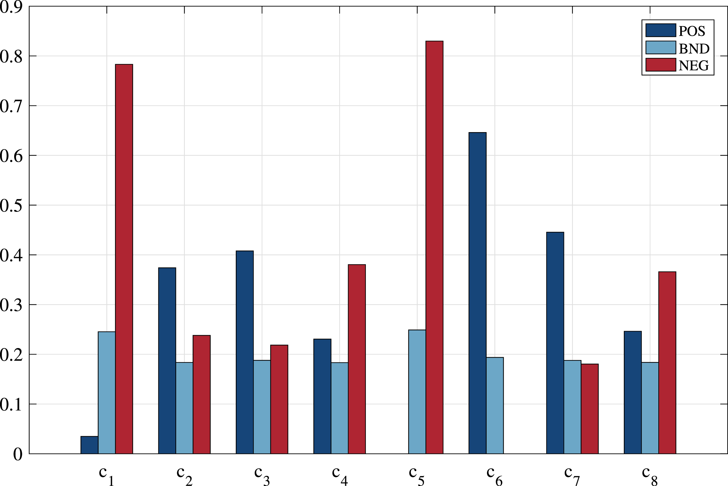
Expected loss and region.

5.2 Comparison analysis

In this section, we compare the division and ranking results of the proposed method with the existing MADM method to test the scientific validity of our method.

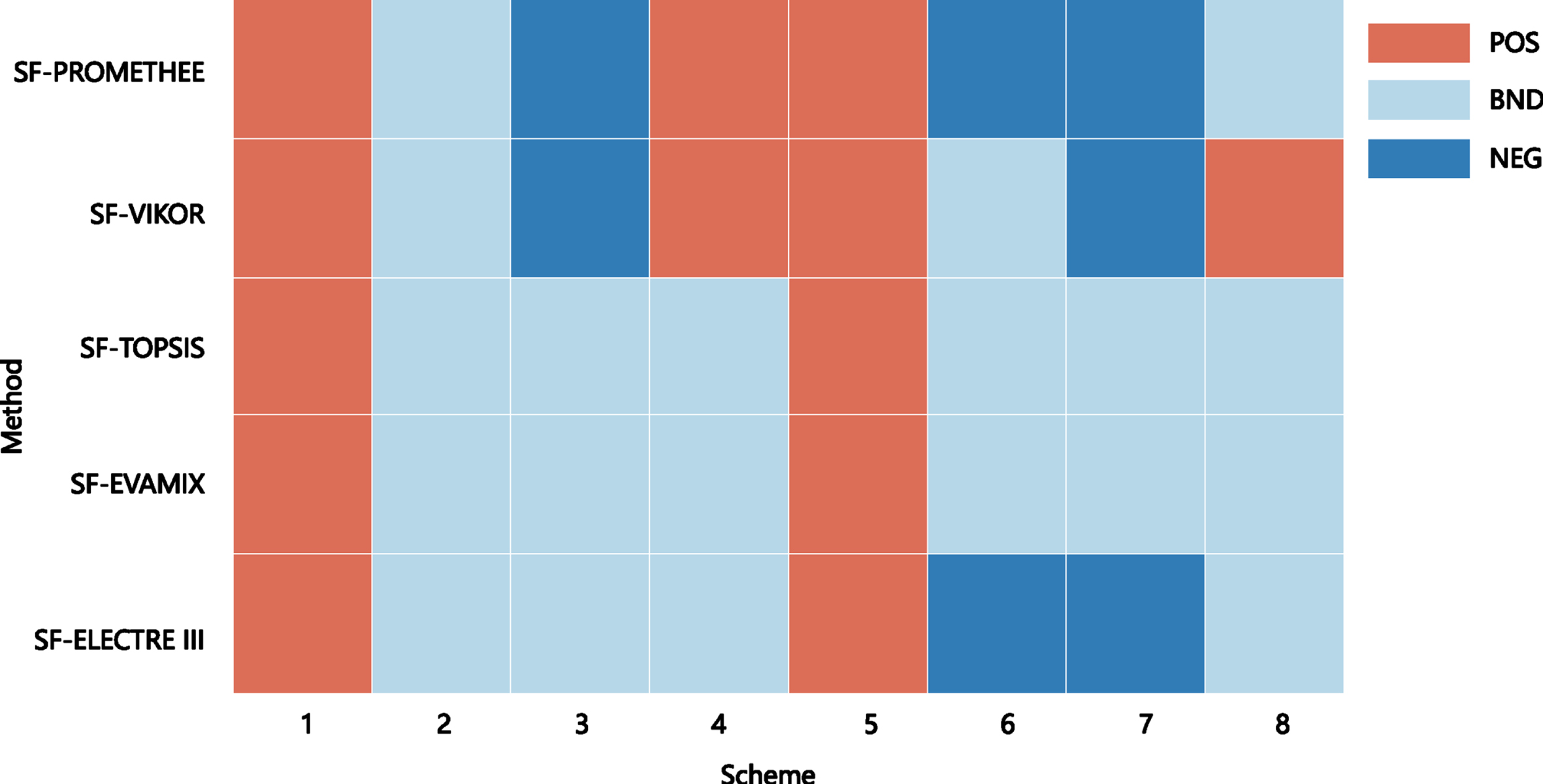
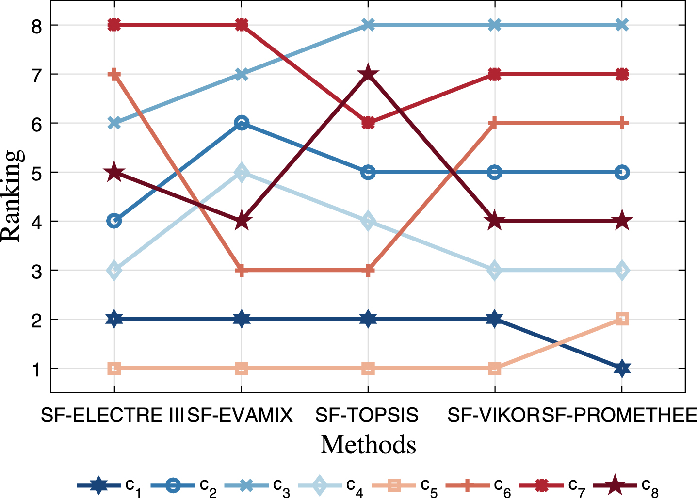
We select SF-EVAMIX-3WD, SF-TOPSIS-3WD, SF-VIKOR-3WD, and SF-PROM ETHEE-3WD methods to compare with the proposed method, and the results of the schemes division and ranking are shown in Tables 22, 23 and Figs. 3, 4. (where the risk aversion coefficients σ are 0.30).

Table 22
Comparison division matrix

Method POS BND NEG

SF-ELECTRE III c₁, c₅ c₂, c₃, c₄, c₈ c₆, c₇

SF-EVAMIX c₁, c₅ c₂, c₃, c₄, c₆, c₇, c₈

SF-TOPSIS c₁, c₅ c₂, c₃, c₄, c₆, c₇, c₈

SF-VIKOR c₁, c₄, c₅, c₈ c₂, c₆ c₃, c₇

SF-PROMETHEE c₁, c₄, c₅ c₂, c₈ c₃, c₆, c₇

Method	POS	BND	NEG
SF-ELECTRE III	c₁, c₅	c₂, c₃, c₄, c₈	c₆, c₇
SF-EVAMIX	c₁, c₅	c₂, c₃, c₄, c₆, c₇, c₈
SF-TOPSIS	c₁, c₅	c₂, c₃, c₄, c₆, c₇, c₈
SF-VIKOR	c₁, c₄, c₅, c₈	c₂, c₆	c₃, c₇
SF-PROMETHEE	c₁, c₄, c₅	c₂, c₈	c₃, c₆, c₇

Table 23

Comparison ranking matrix

Method	RANKING	The best scheme
SF-ELECTRE III	c₅ ≻ c₁ ≻ c₄ ≻ c₂ ≻ c₈ ≻ c₃ ≻ c₆ ≻ c₇	c ₅
SF-EVAMIX	c₅ ≻ c₁ ≻ c₆ ≻ c₈ ≻ c₄ ≻ c₂ ≻ c₃ ≻ c₇	c ₅
SF-TOPSIS	c₅ ≻ c₁ ≻ c₆ ≻ c₄ ≻ c₂ ≻ c₇ ≻ c₈ ≻ c₃	c ₅
SF-VIKOR	c₅ ≻ c₁ ≻ c₄ ≻ c₈ ≻ c₂ ≻ c₆ ≻ c₇ ≻ c₃	c ₅
SF-PROMETHEE	c₁ ≻ c₅ ≻ c₄ ≻ c₈ ≻ c₂ ≻ c₆ ≻ c₇ ≻ c₃	c ₁

Fig. 3

Division in different methods.

Fig. 4

Ranking in different methods.

In terms of division, regardless of the method c₁ and c₅ are always in the POS region, and the rest of the schemes vary due to the differences in the possibility obtained by each method. In terms of ranking, c₁ and c₅ also always occupy the top two places, c₃ and c₇ have records of ranking last, and c₆ ranking changes more unstable.

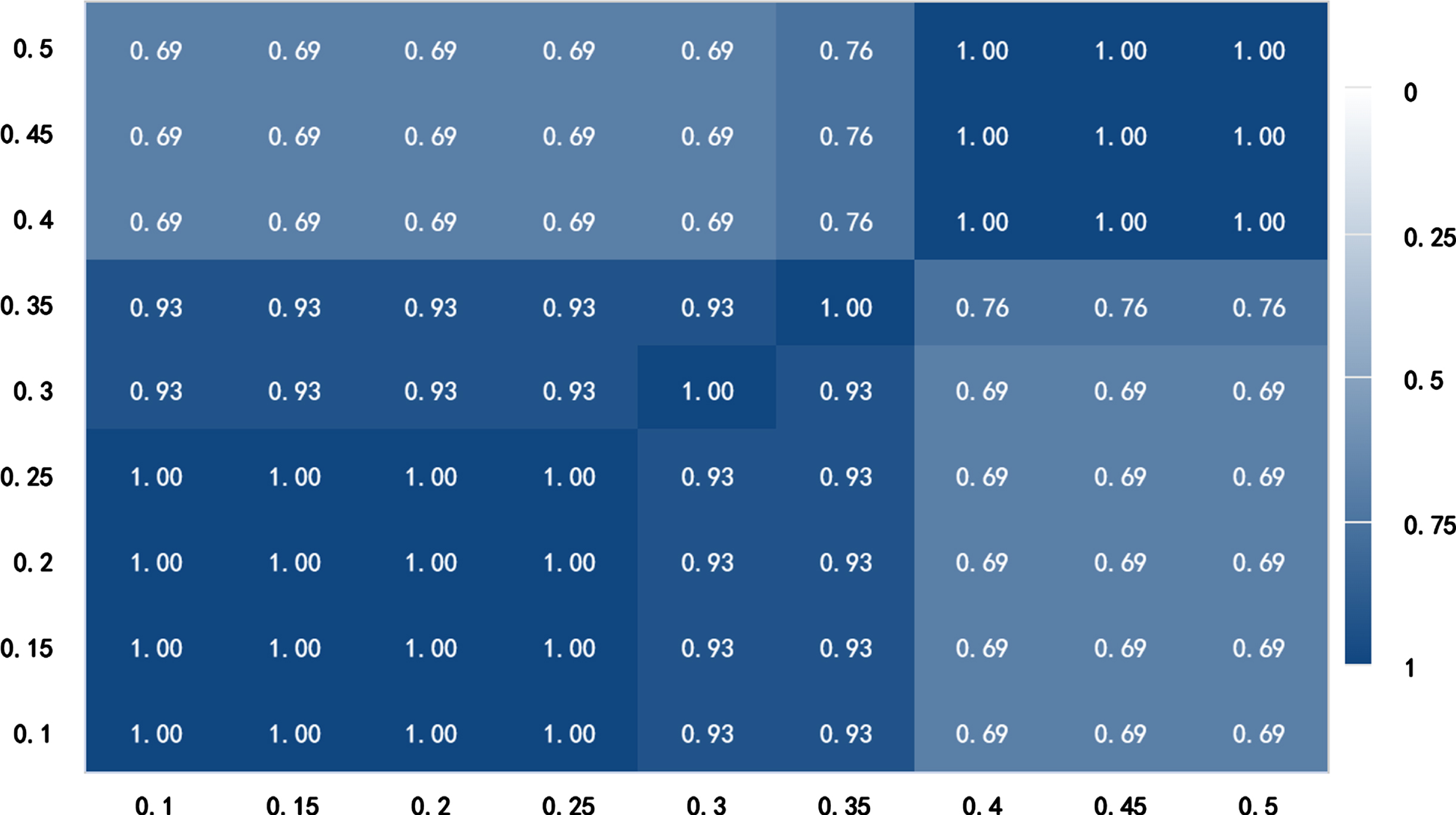
We analyze the ranking of the schemes obtained by several methods by applying the Spearman rank consistency coefficient, as shown in Fig. 5.

Fig. 5

Speraman rank consistency coefficient in different methods.

By checking the table we know that when correlation coefficient >0.643 at n=8 indicates a strong correlation at the confidence interval 95% level.

The correlation coefficient analysis shows that, except for SF-ELECTRE III-3WD and SF-TOPSIS-3WD, the correlation coefficients between the methods are greater than 0.643, which has a strong correlation, indicating that the results of the proposed methods are more reliable.

In addition, when analyzing the Spearman rank correlation coefficient, it is found that SF-TOPSIS-3WD has the lowest average correlation with the remaining four methods, and a comparison of the program rankings revealed that c₈ is only in the last three in SF-TOPSIS-3WD, with a large gap with the remaining results.

Additionally, SF-ELECTRE III-3WD can partition the alternatives evenly in one go compared with the existing method proposed in this paper. Observing the Table 22, it can be seen that the proposed method can quickly eliminate two obvious inferior solutions c₆ and c₇ compared with SF-EVAMIX-3WD and SF-TOPSIS-3WD, while SF-VIKOR-3WD and SF-PROMETHEE-3WD have 3 and 4 solutions respectively in the POS partition, which still have more obvious selection difficulties.

Also, ELECTRE III itself is a non-compensatory MADM method, and in this case, scheme c₆ performs the worst under attribute a₄, and even though scheme c₆ is ranked highly under the remaining attributes, the final result has the inability to be in the top. And through Table 22 we find that both SF-EVAMIX-3WD and SF-TOPSIS-3WD place it in the third place, and in SF-VIKOR-3WD and SF-PROMETHEE-3WD, scheme c₆ is also ranked ahead of SF-ELECTRE III-3WD.

In summary, the consistency of the results obtained by several methods is high, and the proposed method has strong scientific validity. The combination of ELECTRE III and 3WD can be used to quickly eliminate significantly inferior alternatives, resulting in an accurate and efficient decision process, and extending it to a spherical ambiguous environment, which greatly expands its application area, for example, in the most common supplier decision scenario when a supplier has a particular poor attribute, it should be excluded at the first time.

5.3 Sensitivity analysis

Due to the different attitudes of firms towards risk, different values of risk aversion coefficients are derived, yet σ is always between [0.0,0.5]. Different risk aversion coefficients can have an impact on the division results of 3WD, which in turn affects the ranking of customers. Therefore, we analyze the division and ranking results under different σ to find the differences and connections that exist.

We take a minimum σ of 0.10, a maximum σ of 0.50, and the step size of 0.05, then obtained 9 sets of sensitivity analysis results, show in Tables 24, 25 and Figs. 6, 7.

Table 24
Sensitivity analysis division matrix

σ POS BND NEG

0.10 c₁, c₅ c₂, c₃, c₄, c₇, c₈ c ₆

0.15 c₁, c₅ c₂, c₃, c₄, c₇, c₈ c ₆

0.20 c₁, c₅ c₂, c₃, c₄, c₇, c₈ c ₆

0.25 c₁, c₅ c₂, c₃, c₄, c₇, c₈ c ₆

0.30 c₁, c₅ c₂, c₃, c₄, c₈ c₆, c₇

0.35 c₁, c₅ c₂, c₄, c₈ c₃, c₆, c₇

0.40 c₁, c₅ c₄, c₈ c₂, c₃, c₆, c₇

0.45 c₁, c₄, c₅, c₈ c₂, c₃, c₆, c₇

0.50 c₁, c₄, c₅, c₈ c₂, c₃, c₆, c₇

σ	POS	BND	NEG
0.10	c₁, c₅	c₂, c₃, c₄, c₇, c₈	c ₆
0.15	c₁, c₅	c₂, c₃, c₄, c₇, c₈	c ₆
0.20	c₁, c₅	c₂, c₃, c₄, c₇, c₈	c ₆
0.25	c₁, c₅	c₂, c₃, c₄, c₇, c₈	c ₆
0.30	c₁, c₅	c₂, c₃, c₄, c₈	c₆, c₇
0.35	c₁, c₅	c₂, c₄, c₈	c₃, c₆, c₇
0.40	c₁, c₅	c₄, c₈	c₂, c₃, c₆, c₇
0.45	c₁, c₄, c₅, c₈		c₂, c₃, c₆, c₇
0.50	c₁, c₄, c₅, c₈		c₂, c₃, c₆, c₇

Table 25

Sensitivity analysis ranking matrix

σ	Ranking	The best scheme
0.10	c₅ ≻ c₁ ≻ c₄ ≻ c₂ ≻ c₈ ≻ c₇ ≻ c₃ ≻ c₆	c ₅
0.15	c₅ ≻ c₁ ≻ c₄ ≻ c₂ ≻ c₈ ≻ c₇ ≻ c₃ ≻ c₆	c ₅
0.20	c₅ ≻ c₁ ≻ c₄ ≻ c₂ ≻ c₈ ≻ c₇ ≻ c₃ ≻ c₆	c ₅
0.25	c₅ ≻ c₁ ≻ c₄ ≻ c₂ ≻ c₈ ≻ c₇ ≻ c₃ ≻ c₆	c ₅
0.30	c₅ ≻ c₁ ≻ c₄ ≻ c₂ ≻ c₈ ≻ c₃ ≻ c₆ ≻ c₇	c ₅
0.35	c₅ ≻ c₁ ≻ c₄ ≻ c₂ ≻ c₈ ≻ c₆ ≻ c₇ ≻ c₃	c ₅
0.40	c₅ ≻ c₁ ≻ c₄ ≻ c₈ ≻ c₆ ≻ c₇ ≻ c₃ ≻ c₂	c ₅
0.45	c₅ ≻ c₁ ≻ c₄ ≻ c₈ ≻ c₆ ≻ c₇ ≻ c₃ ≻ c₂	c ₅
0.50	c₅ ≻ c₁ ≻ c₄ ≻ c₈ ≻ c₆ ≻ c₇ ≻ c₃ ≻ c₂	c ₅

Fig. 6

Division in different σ.

Fig. 7

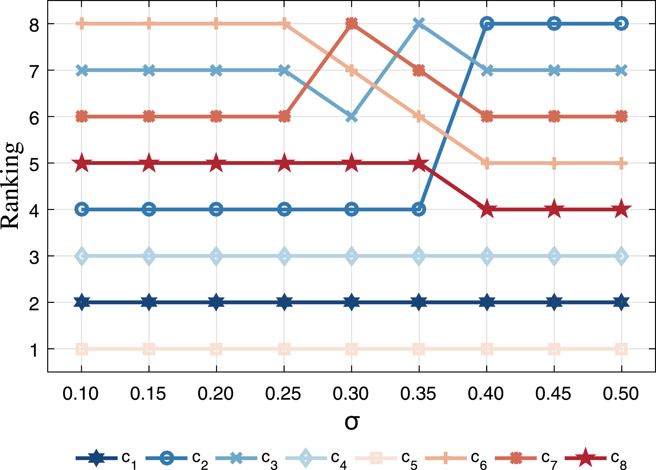
Ranking in different σ.

From the division results, it can be seen that as the risk aversion coefficient σ increases from 0.10 to 0.45, the number of customers in the BND region decreases from 5 to 0, indicating that the larger the σ, the closer the result is to the two-way decision. And in the real decision-making situation, due to the uncertainty and fuzziness of information, we generally take σ = 0.3 as the risk avoidance coefficient. The result in this case is experimentally verified to have a more uniform distribution of programs, which can achieve both the decision-making effect and the actual situation.

By observing the decision results under each σ, we find that when σ is at [0.10,0.25], its division and ranking results are the same, indicating that when σ ≤ 0.25, there are highly similar in its results. When σ is at [0.30,0.35], its division is more uniform and the ranking only changes for c₃, and this interval is also the most widely used in real life. When σ is at [0.40,0.50], its ranking is completely consistent, indicating that when the risk aversion level reaches 80%, it can already produce quite reliable results, and when σ reaches 0.45, its division and ranking results are completely consistent with 0.50.

Regardless of the value of σ, c₁, c₅ always be in the POS region, c₆ always be in the NEG region, and c₅ always be the most desirable customer, so the company should consider prioritizing stocking for c₅ and c₁ to issue.

We analyze the ranking of the schemes obtained by different σ by applying the Spearman rank consistency coefficient show in Fig. 8.

Fig. 8

Ranking in different σ.

By observational analysis we found that the minimum Spearman’s rank correlation coefficient is 0.69, which has reached a confidence level of more than 95%, indicating that the proposed method is insensitive to changes in σ.

6 Conclusion

Compared with the traditional 3WD method, the advantages of the proposed method are as follows.

Firstly, it extends the 3WD theory to the spherical fuzzy environment, which provides an effective solution strategy for the spherical fuzzy environment MADM problems. Also providing a broader space for the application of 3WD. Secondly, ITARA provides a subjective-objective concurrent assignment method for the spherical fuzzy MADM, which considers the relationship between decision information and also incorporates the expert’s cognitive provisions for the differences among attributes, which is more effective. Thirdly, ELECTRE III is a MADM method based on the pairwise comparison, which makes the schemes possess weaker compensations and facilitates the selection of the best solution because it considers both consistency measures and inconsistency measures, and the latter are handed strict for the attribute requirements of the solutions. In this paper, we used the Hamming distance between the SFN and the ideal decision information to determine its dominant relationship, which avoids the destruction of the original information in the process of defuzzification. Finally, the improvement of 3WD also gives each scheme the loss function matrix derived from itself, which is more relevant to the description of each scheme, and the addition of risk avoidance coefficient σ upgrades the risk avoidance function of 3WD to ensure the scientificity of the decision results.

The traditional MADM problem tends to be customer-centric in its selection of suppliers. However, the encroachment of COVID-19 has brought far-reaching impacts to both suppliers and customers, and suppliers have to consider the feasibility of cooperation in the present moment when serving customers, which creates a new MADM problem. The method proposed in this paper effectively solves this problem, and we believe our method will be applied more widely in the future.

Even though we have improved the credibility of the overall results by improving each method when constructing the model, the determination of the undifferentiated threshold in ITARA, the determination of the superiority and inferiority relationships among the evaluated information in ELECTRE III, and the distance measure used in the loss function acquisition can affect the decision effect to varying degrees. In the future research, we will investigate the range of undifferentiated limits among attributes, and then propose a combined subjective and objective method for determining undifferentiated thresholds, and at the same time, evaluate the distance measure of SFNs to determine its more accurate method for evaluating the superiority and inferiority of decision information, and further expand the method for determining the loss function in a spherical fuzzy environment.

References

Yao

Y.Y.

, Three-way decision: an interpretation of rules in rough set theory, International Conference on Rough Sets and Knowledge Technology (2009), 642–649.

Hatefi

M.A.

, Indifference threshold-based attribute ratio analysis:A method for assigning the weights to the attributes in multiple attribute decision making, Applied Soft Computing 74(2019), 643–651.

Roy

, The outranking approach and the foundations of ELECTREmethods, Theory and Decision 31 (1991), 49–73.

Mahmood

, Kifayat

, Khan

and Jan

, An approach towarddecision-making and medical diagnosis problems using the concept ofspherical fuzzy sets, Neural Computing and Applications 31 (2019), 7041â£″7053.

Zadeh

L.A.

, Fuzzy sets, Information and Control 8(1965), 338–356.

Atanassov

K.T.

, Intuitionistic fuzzy sets, Fuzzy Sets andSystems 20 (1986), 87–96.

Yager

R.R.

, Pythagorean fuzzy subsets, Proceedings of Joint IFSA World Congress and NAFIPS Annual Meeting, Edmonton, Canada (2013), 57–61.

Cuong

B.C.

, Picture fuzzy sets, Journal of Computer Science and Cybernetics 30 (2015), 409.

Yildirim

B.F.

and Kuzu Yıldırım , Evaluating thesatisfaction level of citizens in municipality services by usingpicture fuzzy VIKOR method: –period analysis, Decision Making: Applications in Management and Engineering 5(2022) (2019), 50–66.

10.

Das

A.K.

and Granados

, FP-intuitionistic multi fuzzy N-soft setand its induced FP-Hesitant N soft set in decision-making, Decision Making: Applications in Management and Engineering 5(2022), 67–89.

11.

Riaz

and Athar Farid

H.M.

, FPicture fuzzy aggregation approachwith application to third-party logistic provider selection process, Reports in Mechanical Engineering 5 (2022), 227–236.

12.

Ashraf

, Ullah

, Hussain

and Bari

, Interval-valued picture fuzzy maclaurin symmetric mean operator with application in multiple attribute decision-making, Reports in Mechanical Engineering 3 (2022), 210–226.

13.

Cao

H.F.

, Zhang

R.T.

and Wang

, Some spherical linguistic Muirhead mean operators with their application to multi-attribute decisionmaking, Journal of Intelligence and Fuzzy Systems 37(2019) (2019), 8079–8111.

14.

Zeng

S.Z.

, Munir

, Mahmood

and Naeem

, Some T-Spherical fuzzy einstein interactive aggregation operatorsand their application to selection of photovoltaic cells, Mathematical Problems in Engineering 2020(2020), 1–16.

15.

Liu

P.D.

, Zhu

B.Y.

, Wang

and Shen

M.J.

, An approach based onlinguistic spherical fuzzy sets for public evaluation of sharedbicycles in China, Engineering Applications of ArtificialIntelligence 87 (2020), 103295.

16.

Zižović

and Pamucar

, New model for determiningcriteria weights: Level Based Weight Assessment (LBWA) model, Decision Making: Applications in Management and Engineering 2(2019), 126–137.

17.

Pamucar

, Stević

Ž.

and Sremac

, NA new model fordetermining weight coefficients of criteria in MCDM models: Fullconsistency method (FUCOM), Symmetry 10 (2018), 393.

18.

Sofuoglu Alper

, Development of an ITARA-based hybridmulti-criteria decision-making model for material selection, Soft Computing 23 (2019), 6715–6725.

19.

Ulutas

and Karabašević

, Development of a Novel Integrated CCSD-ITARA-MARCOS Decision-Making Approach for Stackers Selection in a Logistics System, Mathematics 8 (2020), 1672.

20.

Liu

P.D.

, Pan

and Xu

H.X.

, Multi-attributive border approximation area comparison (MABAC) method based on normal q-rung ortho pairfuzzy environment, Journal of Intelligence AND Fuzzy Systems 40 (2021), 9085–9111.

21.

Roy

, Me’todologie multicrite‘re d’aide la decision, Collection Gestion, Paris, Economica (1985).

22.

Yadav

and Luthra

, A framework to overcome sustainable supply chain challenges through solution measures of industry 4.0 and circular economy: An automotive case, Journal of Cleaner Production 254 (2020), 112–120.

23.

Zhou

L.P.

, Wan

S.P.

and Dong

J.Y.

, A fermatean fuzzy ELECTRE methodfor multi-criteria group decision-making, Informatica 33(2022), 181–224.

24.

Liu

Z.M.

, Bi

Y.W.

, Wang

X.Y.

, Sha

L.B.

and Liu

P.D.

, A generalized TODIM-ELECTRE II method based on linguistic Z-numbers and Dempster–Shafer evidence theory with unknown weight information, Complex AND Intelligent Systems 8 (2022), 941–971.

25.

Chen

Z.S.

, Zhang

, Rodríguez

R.M.

, Pedrycz

and Martínez

, Expertise-based bid evaluation forconstruction-contractor selection with generalized comparativelinguistic ELECTRE III, Automation in Construction 125(2021), 103578.

26.

Peng

H.G.

, Shen

K.W.

, He

S.S.

, Zhang

H.Y.

and Wang

J.Q.

, Investmentrisk evaluation for new energy resources: An integrated decisionsupport model based on regret theory and ELECTRE III, EnergyConversion and Management 183 (2019), 332–348.

27.

Akram

, Ilyas

and Al-Kenani

A.N.

, Two-phase group decision-aiding system using ELECTRE III Method in Pythagorean Fuzzy Environment, Arabian Journal for Science and Engineering 46 (2021), 3549–3566.

28.

Mahmoudi

, Aydi

and Ibrahim

, Site selection for artificial recharge with treated wastewater with the integration of multi-criteria evaluation and ELECTRE III, Environmental Science and Pollution Research 28 (2021), 46748–46763.

29.

Chen

Z.S.

, Zhang

, Rodríguez

R.M.

, et al. Expertise-based bidevaluation for construction-contractor selection with generalizedcomparative linguistic ELECTRE III, Automation in Construction 125 (2021), 103578.

30.

Pawlak

, Rough sets, International Journal of Computer ANDInformation Sciences 11 (1982), 341–356.

31.

Lang

and Miao

, Three-way group conflict analysis based on Pythagorean fuzzy set theory, IEEE Transactions on Fuzzy Systems 28 (2020), 447–461.

32.

, Xu

Z.S.

and Wang

, Three-way decisions based on some Hamacher aggregation operators under double hierarchy linguistic environment, International Journal of Intelligent Systems 36 (2021), 7731–7753.

33.

Wang

, Li

, Qian

, Huang

and Zhou

, A regret-basedthree-way decision model under interval type-2 fuzzy environment, IEEE Transactions on Fuzzy Systems 30 (2020), 175–189.

34.

Sałabun

, Watróbski

and Shekhovtsov

, re MCDA MethodsBenchmarkable? A Comparative Study of TOPSIS, VIKOR, COPRAS, andPROMETHEE II Methods, Symmetry 12 (2020), 1549.

35.

Corazza

, Funari

and Siviero

, A murame-based technology forbank decision support in credit worthiness assessment, Banks and Bank Systems 9 (2014), 8–18.

ITARA and ELECTRE III three-way decision model in the spherical fuzzy environment and its application in customer selection

Abstract

Keywords

1 Introduction

2 Literature review

3 Preliminary knowledges

3.1 Spherical fuzzy sets and spherical fuzzy numbers

Table 1 Loss matrix A ¬A a P λ PP λ PN a B λ BP λ BN a N λ NP λ NN

5.1 Numerical example in SF-ITARA-ELECTRE III-3WD

Table 22 Comparison division matrix Method POS BND NEG SF-ELECTRE III c1, c5 c2, c3, c4, c8 c6, c7 SF-EVAMIX c1, c5 c2, c3, c4, c6, c7, c8 SF-TOPSIS c1, c5 c2, c3, c4, c6, c7, c8 SF-VIKOR c1, c4, c5, c8 c2, c6 c3, c7 SF-PROMETHEE c1, c4, c5 c2, c8 c3, c6, c7

References

Table 1
Loss matrix

A ¬A

a _P λ_PP λ_PN

a _B λ_BP λ_BN

a _N λ_NP λ_NN