A mobile robot path planning using improved beetle swarm optimization algorithm in static environment

Abstract

Optimization problems in the field of industrial engineering usually involve massive amounts of information and complex scheduling process with the characteristics of high-dimension and non-convexity, which bring many challenges to finding an optimal solution. We proposed an improved beetle swarm optimization (IBSO) algorithm demonstrating the potential to solve different problems of path planning in static environment with good performance. Firstly, the algorithm is an upgrade of the original beetle antennae search (BAS) algorithm and the search strategy is improved by replacing a single beetle by multiple beetles. Secondly, the global search ability gets enhanced, and the diversity of optimization is improved through introducing nonlinear sinusoidal disturbance with Levy flight mechanism in beetles’ position. Finally, the search performance of beetle swarm is improved by simulating the characteristics of employment bees to search for a better solution near the honey source field in the Artificial Bee Colony (ABC) algorithm. Our experiment results show that IBSO algorithm can achieve higher search efficiency and wider search ranges through well balancing the advantages of local search and fast optimization of the BAS algorithm with the global search of the improved mechanism. The IBSO algorithm has shown the potential to provide a new solution for several optimization problems in path planning in static environment.

Keywords

Path planning beetle antennae search algorithm Levy flight artificial bee colony algorithm

1 Introduction

In recent years, unmanned aerial vehicles (UAV) and industrial mobile robots have developed rapidly, and their applications have been expanding in many scientific and technological fields, such as Disaster monitoring [1, 2], water resources inspection [3, 4], power system monitoring [5], meteorological detection [6] and etc. It can be seen that the development of related technologies for UAV and industrial robots plays an increasingly important role in these areas. How to choose the optimal running trajectory and how to avoid obstacles in time for these intelligent technologies such as UAV and industrial mobile robots during the execution of tasks has attracted the attention of many researchers. Determining a reasonable path planning plan scheme is the primary focus of the researchers’ attention. The path planning problem can be solved by searching for the optimal solution of the optimization problem through the optimization algorithms.

Path planning is a branch of research on motion planning where the sequence point set or curve connecting the source and destination is called the path, and the sequence arrangement strategy of the sequence point set is called path planning. A reasonable planning strategy can save a lot of cost. Path planning includes several types of optimization problems. Based on the characteristics of the data used, path planning can be divided into discrete domain and continuous domain. One of the most classical optimization problems in path planning is the traveling salesman problem that falls into the category of the ergodic optimal path problem in the discrete domain. It is also a type of one-dimensional static optimization problem, equivalent to the route optimization problem after the environmental information is simplified, widely used in printed-circuit board hole turning [7], logistics problems [8] and various vehicle problems [9]. The common methods to solve such path problems are exact algorithms, including Dynamic Programming (DP) method [10] and Branch and Bound method [11]. However, as the scale of the problem increases, the exact algorithm will become powerless.

The goal of the global path planning in a continuous domain is to avoid obstacles and find the shortest path to the destination in the safe range when the environmental information is known and static. It is an optimization in the continuous multidimensional static environment. This type of path planning is mainly applied to the path planning for unmanned aerial vehicle [12], Cruise missile trajectory planning [13] and robot manipulator autonomous movement path planning [14]. The traditional algorithms for solving this kind of path planning problems mainly include Artificial Potential Field (APF) [15], A* algorithm [16], etc. The traditional APF algorithm is a virtual force method. It imitates the movement of objects under gravitational and repulsive forces. The path is optimized by establishing the gravitational and repulsive field function. In the process of path planning, it is easy to fall into a certain local area and cannot reach the destination. The A* algorithm is a direct search method for solving the shortest path in a static road network. The closer the distance estimation value in the algorithm is to the actual value, the faster the final search speed, but the effectiveness of A* algorithm is not ideal and there exist a large number of turns in the path. The Rapidly-Exploring Random Tree (RRT) algorithm [17] uses collision detection on sampling points in the state space and directs the search to a blank area to find a planned path from the starting point. However, due to the limitations of the algorithm, the randomness of the next step of the search is too large, making the path unsmooth. Traditional algorithms often have difficult modeling problems when solving practical problems, while graphics methods provide a basic modeling method. The Grid method [18] is a method of map modeling, which divides the environmental space into units and represents them with squares of equal size. The selection of the grid size is an important factor affecting the performance of the planning algorithm.

The intelligent optimization algorithms are inspired by nature, and they play a very good role when dealing with path planning problems under complex and dynamic environmental information. The emergence of intelligent optimization algorithms provides a new calculation method for solving path planning problems. This type of method does not need to construct a complex mathematical model to obtain a globally feasible path planning solution. Researchers have proposed many heuristic optimization algorithms for solving path planning problems by simulating natural biological evolution or group behavior, such as Bat Algorithm (BA) [19], Firefly Algorithm (FA) [20], Particle Swarm Optimization (PSO) Algorithm [21] etc. Gemeinder. et al. proposed a mobile robot based on Genetic Algorithm (GA) [22], and introduced an active search algorithm to overcome the shortcomings of the earlier version. Wu et al. proposed a novel Beetle Antennae Algorithm with fallback mechanism [23]. If a collision occurs, it will fall back a certain distance, which results in the increase of the solving time and leads to poor optimization results after back-off. Wu et al. proposed an Agglomerative Greedy Brain Storm Optimization (AG-BSO) Algorithm [24] to solve typical cases in traveling salesman problem (TSP) and obtained better results. Zhong et al. proposed a discrete pigeon-inspired optimization algorithm with metropolis acceptance criterion [25] which performs well in TSP with a large-scale urban dimension. To sum up, the intelligent optimization algorithm can help improve the accuracy of path planning and each algorithm has its own advantages and disadvantages when solving such problems. The research on the path planning has never stopped.

The BAS algorithm is one of the intelligent optimization algorithms. The advantage of this algorithm is that only one individual beetle is used for search and optimization, which reduces the amount of computation to a certain extent. Because of its simple mechanism, the algorithm converges fast. Since BAS uses an individual beetle, it is very easy to cause the beetle to reach local extreme value in the search domain, resulting in inaccurate solution results. At the same time, in each position update of BAS algorithm, the beetle flies in a straight line along the tentacle direction, which is also one of the factors that make BAS easy to enter the local extreme value range. To solve the above problems, we proposed the IBSO algorithm that enhances the BAS algorithm and combines it with the swarm intelligence optimization algorithm. The individual beetle search and optimization is advanced to the beetle swarm for search and optimization. Combined with the idea of hiring bees to search near the nectar source neighborhood in the artificial bee colony (ABC) algorithm, it enriches the search ability of the beetle swarm to solve the global problem. Finally, the Levy flight strategy with nonlinear sinusoidal disturbance is introduced to address the shortcomings of the BAS algorithm that the beetle must fly directly when the position is updated. The beetles now can fly randomly according to the step length. Compared with the ABC and BAS algorithms, the IBSO algorithm has a powerful search range and faster search speed. The main contributions of our algorithm are listed as follows:

Changing individual beetle search into beetle swarm search, and employing the ABC algorithm where bees searching in the nectar source neighborhood to enrich the search range.

Introducing the Levy flight strategy with nonlinear sinusoidal disturbance, so that the beetle has the ability of random flight, so as to change the defect that the beetle flies in a straight line along with the tentacle direction during each position update.

The proposed algorithm has been applied to solve several optimization problems in path planning, including the TSP and obstacle avoidance path planning problem. The simulations have shown good performance.

The rest of the paper is organized as follows. In section 2, we introduce the basic problem models of two types of path planning applications. In section 3, we introduce the design of the IBSO algorithm. In section 4, we use the benchmark function to test and verify the IBSO algorithm and show the algorithm flowchart. In section 5, we introduce the verification and application of IBSO in path planning of mobile robots in static environment, show the simulation results, and compare the performance of IBSO and counterpart algorithms in path planning. In section 6, we analyze the shortcomings of the IBSO and the focus of the next work. In section 7, we summarize the whole paper.

2 Problem Model

Path planning has a wide range of applications. In this paper, we mainly discuss and analyze two kinds of optimization problems: ergodic optimal path problem in a discrete domain and global path planning problem in a continuous domain.

2.1 Ergodic optimal path problem in discrete domain

The general characteristic of ergodic optimal path problem in discrete domain is that the path information is static, with the starting point as the final target node. There might be multiple sub target nodes in the middle. The motion actuator is required to start from the starting point with the shortest path, traverse all sub target nodes, and return to the starting point. This kind of problem mainly includes TSP and its extended application.

2.1.1 Optimization of TSP

The traveling salesman problem [26], also known as the salesman problem, is a typical NP-hard problem. Given n city coordinate locations and distances between cities, a traveling salesman starts from a point city, traverses other cities, visits each city only once and finally returns to the originating city, and ensures the shortest total path length. The mathematical model of TSP is described as follows:

Set G = (V, E) is the weighted graph, V = {v₁, v₂, . . . , v_n} is the vertex set, E is the edge set, the distance between vertex i and j is d_ij, it is known that d_ij > 0, i, j ∈ V, and set x_ij represents the sub-path form the i–th city to the j–th city. If x_ij exists in the path of the travel agent, then x_ij = 1,otherwise x_ij = 0. Its mathematical expression is as follows: $x_{ij} = {\begin{matrix} 1, optimal path (i, j) \in L \\ 0, other situations \end{matrix}$ (1)

L is the solution sequence, then the optimal representation of the traversal path of the TSP problem can be written as a linear programming form as follows: $Min Z (L) = \sum_{i \neq j} d_{ij} x_{ij}$ (2) $s . t . {\begin{matrix} \sum_{i \in V, i \neq j} x_{ij} = 1 i \in V \\ \sum_{j \in V, j \neq i} x_{ji} = 1 j \in V \\ \sum_{i, j \in L} x_{ij} ⩽ | L | - 1, \forall L \subset V, 2 ⩽ | L | ⩽ n - 1 \\ x_{ij} \in {0, 1} \end{matrix}$ (3)

In the Equation (3), |L| is the number of elements in the set L. The constraint condition in the Equation (3) is that each vertex has and can only be traversed once, and that Hamilton does not have any subtour. Find the one with the lowest weight among all Hamilton path satisfying the condition. After the traveling salesman walks through all the cities, set its traversal path is L = (x₁, x₂, . . . , x_n, x₁), that is, the order of the traveling salesman’s travel cities. The above problem is transformed into determining a traversal sequence (x₁, x₂, . . . , x_n, x₁) and finding its minimum value. $min Z (L) = \sum_{i = 1}^{n - 1} d (x_{i}, x_{i + 1}) + d (x_{n}, x_{1})$ (4)

The optimal path conversion mechanism of the single TSP is shown in Fig. 1:

Fig. 1

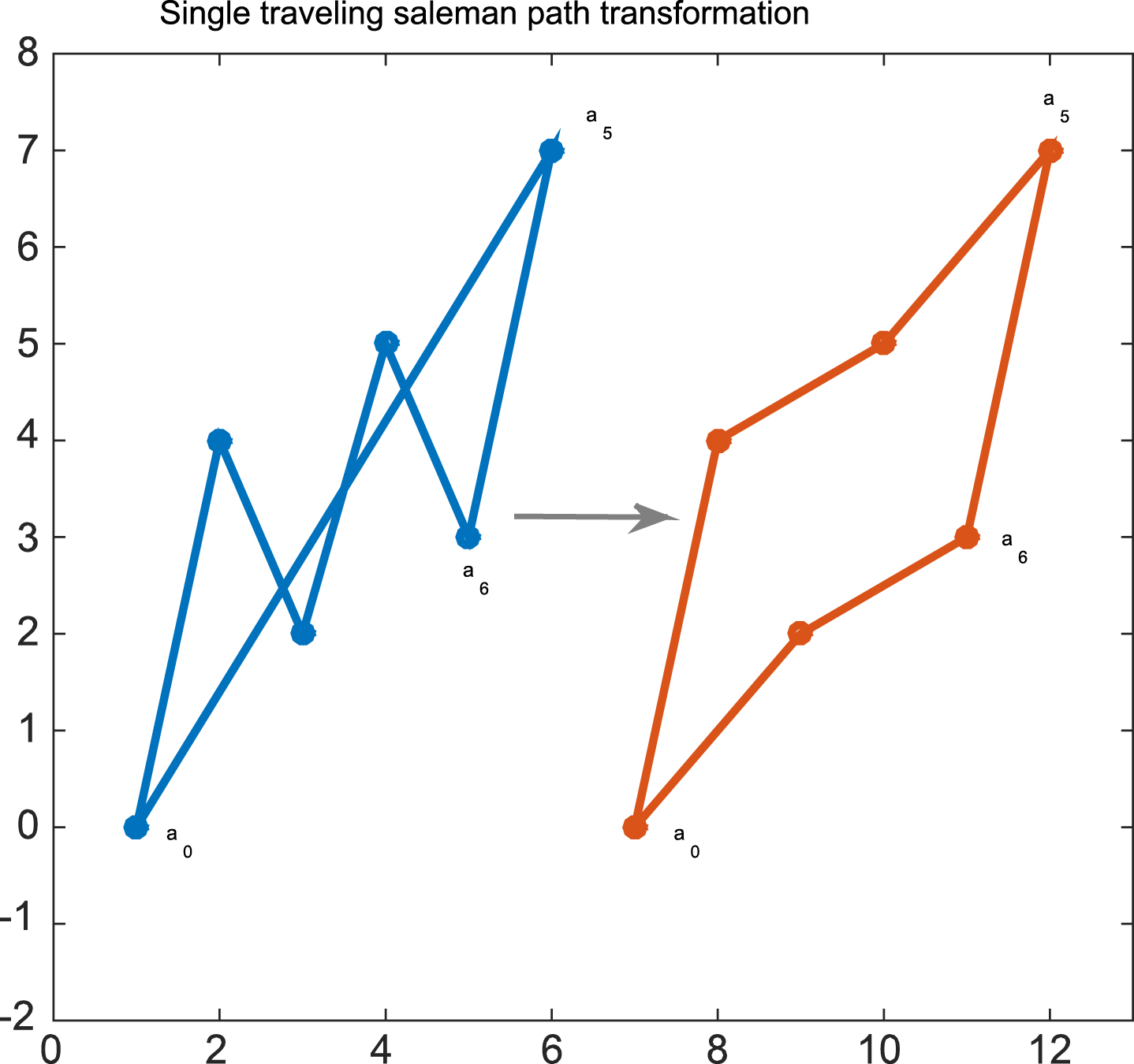
Single traveling salesman path conversion.

2.1.2 Optimization of MTSP

The Multiple Traveling Salesman Problem (MTSP) is a generalization of the classic traveling salesman problem, which is to transform a single traveling salesman into multiple traveling salesman, and add some additional conditions to make it more in line with the problems of vehicle path planning [27], emergency material distribution [28], UAV coverage search [29], and off-grade product control [30] in real life, that is, given cities, traveling salesmen from the same (or different) cities and take a travel route respectively, so that each city has one and only one traveling salesman (except the departure city), and at the same time, the total distance traveled by all traveling salesmen is required to be as small as possible and the length of the longest loop is as small as possible. Compared to TSP, MTSP has a broader engineering background. Therefore, how to solve MTSP quickly and effectively has high practical application value. The mathematical model of MTSP is as follows:

Point a₀ is used to represent the departure city of the traveling salesman, also known as the source point, A = {a₁, a₂, . . . , a_n-1, a_n} indicates that the cities that m traveling salesman b₁, b₂, . . . , b_m need to visit. Define variables: $x_{ij}^{k} = {\begin{matrix} 1, Traveler b_{k} arrives at city a_{i} from city a_{j} \\ 0, Otherwise \end{matrix}$ $y_{i}^{k} = {\begin{matrix} 1, Traveler b_{k} visits city a_{i} \\ 0, Otherwise \end{matrix}$

Modelling the multiple traveling salesman problem: $min fitness = (\sum_{k = 1}^{m} z_{k})$ (5)

In Equation (5), fitness is the objective function formula, expressed as the minimum total distance of mtraveling salesman, where: $z_{k} = \sum_{i = 0}^{n} \sum_{j = 0}^{n} c_{ij} x_{ij}^{k}, k = 1, 2, . . ., m$ (6)

Equation (6) represents the respective distances of the traveling salesman, where c_ij represents the distance it takes for the traveling salesman to pass through the corresponding arc segment (i, j). The qualifications are: $\sum_{k = 1}^{m} y_{ki} = {\begin{matrix} m, i = 0 \\ 1, i = 1, 2, . . ., n \end{matrix}$ (7)

Equation (7) indicates that starting from the designated city a₀, all cities have one and only one traveling salesman to make a visit. $\sum_{i = 0}^{n} x_{ij}^{k} = y_{j}^{k}, \forall j = 0, 1, . . ., n; k = 1, 2, . . ., m$ (8) $\sum_{j = 0}^{n} x_{ij}^{k} = y_{i}^{k}, \forall i = 0, 1, . . ., n; k = 1, 2, . . ., m$ (9)

Equation (8) indicates that the end city of any arc has only one starting point connected to it. Equation (9) indicates that the starting city of any arc has only one ending city connected to it.

The optimal path conversion mechanism of the MTSP is shown in Fig. 2:

Fig. 2

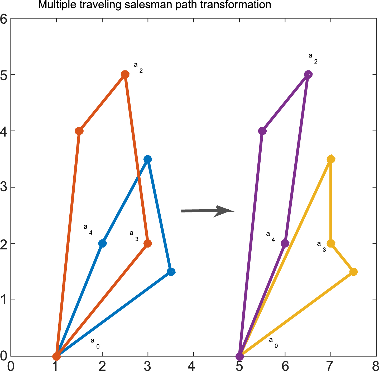
MTSP conversion.

2.2 Global path planning in continuous domain

The global path planning in continuous domain is focused on how to avoid obstacles and find the shortest path to the destination within the safe range when the environmental information is known and static. Solving such problems usually depends on the combination of intelligent algorithms and environment modeling.

2.2.1 2D obstacle avoidance path planning

With the development of new high tech, the application of robots in the field of industrial manufacturing has become more and more extensive, and the path planning of intelligently controlled mobile robots to avoid obstacles during motion has become an important research focus [31]. Traditional obstacle avoidance algorithms include artificial potential field method, A* algorithm, etc.; Intelligent optimization algorithms can also solve obstacle avoidance problems, such as chicken swarm algorithm [32], wolf swarm algorithm [33], etc. The path planning trajectory space modeling of obstacle avoidance problem is as follows:

The intelligent control robot is set to move in a 2D static space environment. In the inertial coordinate system Oxy, the starting point is S, and the target end point is E. There are many obstacles between the two points S and E, and the SE direction is the movement direction of the robot. Connect SE to divide SE into D + 1 equal parts, denoted as se_i, i = (1, 2, . . . , D + 1), in each small segment, make the vertical line l_isegment of se_i, i = (1, 2, . . . , D + 1). Take a point on each vertical line segment l_i to obtain a set of points p = {S, E₁, E₂, . . . , E_D, E} including the starting point and the target end point, and connect these points one by one to form a path. Therefore, the obstacle avoidance problem is classified as solving the optimization coordinate problem, and the optimal path is the optimal fitness value of the optimization problem. Its model diagram is shown in Fig. 3:

Fig. 3

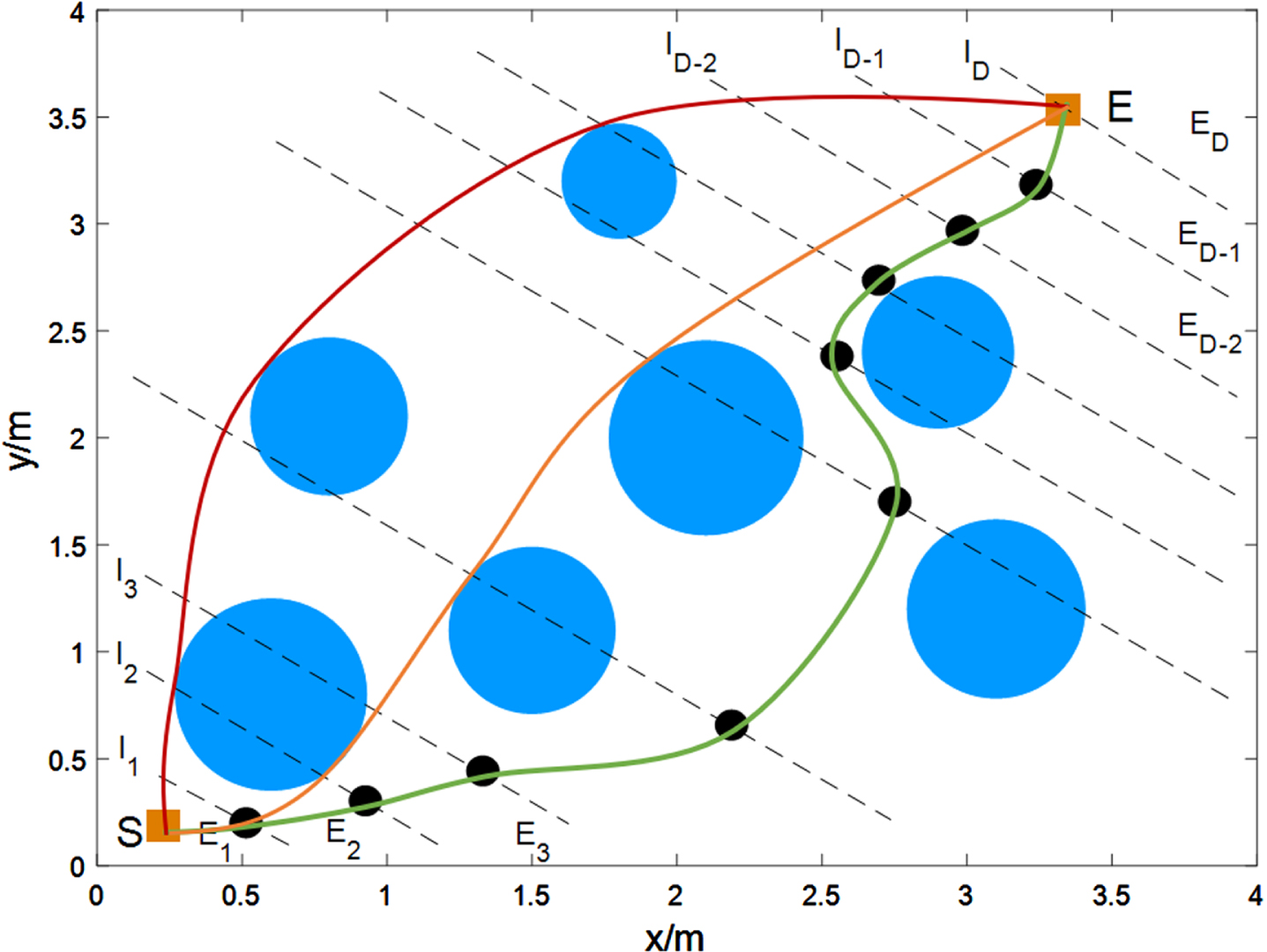
Obstacle avoidance problem space model.

In order to speed up the execution of the algorithm, the line segment SE is used as the x-axis of the coordinate system to denote , and we perform the coordinate transformation on the point set [34], then take SE as the angle γ between the x-axis and the original coordinate axis, and according to the point S as the reference point rotates a clockwise γ, and then translates the origin of the coordinates to realize the coordinate transformation. Through coordinate transformation, the corresponding relationship between the original coordinate system and the local coordinate with SEas the coordinate axis is shown in Equation (10):

$[\begin{matrix} x \\ y \end{matrix}] = [\begin{matrix} cos γ \sin γ \\ - sin γ \cos γ \end{matrix}] [\begin{matrix} x^{'} - x_{s} \\ y^{'} - y_{s} \end{matrix}]$ (10)

Where, represents the coordinates of the corresponding point after coordinate transformation, and (x_s, y_s) represents the coordinates of the initial point S. From the figure, the distance between two parallel lines (l_i, l_i-1) is: $Δ d = \frac{| SE |}{(D + 1)}$ (11)

The movement distance of the robot affects its movement time. Through the fitness function f, the shortest value of the total path length from the starting point to the end point can be obtained. The trajectory distance of the robot movement is: $f = \sum_{i = 1}^{D + 1} \sqrt{(Δ d)^{2} + (y_{i} - y_{i - 1})^{2}}$ (12)

Therefore, the solution of the robot obstacle avoidance path planning problem can be transformed into the extreme value problem of the objective function. When the function Fitness reaches the minimum, the obstacle avoidance path planning problem is completed. The objective function is the fitness function: $min Fitness = f$ (13)

When the robot moves into the obstacle range, it need to adjust the moving direction of the robot to avoid entering the threat area. T is the adjustment function. When a line segment on the moving path collides with the center of the obstacle and the radius of the circle, the robot’s motion trajectory is changed by multiplying the adjustment function by an adjustment factor. $T = \sum_{i = 1}^{D + 1} δ α_{i}$ (14)

In Equation (14), α_i is the number of intersections between the i–th component path and the obstacle object. It can be obtained that the evaluation index of the obstacle avoidance problem is shown in Equation (15), which is used as a performance reference for the obstacle avoidance problem of the intelligent control robot. That is to find the shortest path of the mobile robot without touching the obstacle after entering the threat area. $Z = Fitness + T$ (15)

2.2.2 3D obstacle avoidance path planning

To study the problem of path planning, first of all, we need to model the environment of the planning space, and set the motion area as a 3D space with a size of a * b * c m³ under the rectangular coordinate system. The fitness function is an important index to evaluate the path quality. For the 3D path planning of UAVs, the trajectory cost and the obstacle avoidance cost need to be comprehensively considered.

The trajectory cost f_vis determined by the length of the path fitted by the cubic B-spline curve. Equation (16) represents all adjacent nodes (x_i, y_i, z_i) and (x_i+1, y_i+1, z_i+1) in the path sum of distances.

$\begin{matrix} f_{v} = \sum_{i = 1}^{m} \\ \sqrt{(x_{i + 1} - x_{i})^{2} + (y_{i + 1} - y_{i})^{2} + (z_{i + 1} - z_{i})^{2}} \end{matrix}$ (16)

The minimum distance between the path and the obstacle peak is d_min, which requires a safe distance d_s between the path and the obstacle peak, and the obstacle cost f_a is shown in Equation (17).

$f_{a} = {\begin{matrix} 0, d_{min} ⩾ d_{s} \\ \infty, d_{min} < d_{s} \end{matrix}$ (17)

Combining the trajectory cost and the obstacle avoidance cost, the fitness function is obtained as shown in Equation (18). When d_min ⩾ d_s, the UAV has no collision risk, and the obstacle avoidance cost can be ignored; when d_min < d_s, the UAV has no collision risk. There is a risk of collision, and the fitness function fis infinite.

$f = f_{v} + f_{a}$ (18)

3 Algorithm design and improvement

In this section, we presented the design of IBSO algorithm in depth, including the original BAS algorithm and the optimization strategies introduced. The selection of parameters involved in the algorithm is also described.

3.1 Beetle antennae search algorithm

The BAS algorithm [35] is a heuristic optimization algorithm proposed by Jiang and Li in 2018. The algorithm principle is: food is the target object, and the smell of food is equivalent to a function. Each point value of the function in the space is different. The two antennae of the beetle are able to collect the odor value of two nearby points. The purpose of the beetle is to search the point with the largest odor in the space. The specific orientation of the food is equivalent to the maximum point of the objective function, and the beetle moves step by step to the orientation where the food smells the most. BAS is different from other optimization algorithms in that it only depends on one individual to search, that is, one beetle, which greatly reduces the computation and shortens the computational time. Therefore, the process of beetle foraging is the optimization process of BAS algorithm. The specific steps are as follows:

1). Set the direction vector and step length of the initial position of beetle:

$\vec{dir} = \frac{rands (Dim, 1)}{∥ rands (Dim, 1) ∥}$ (19)

${step}_{t + 1} = eta * {step}_{t} (t = 1, 2, . . ., n)$ (20)

Whererands (•) is the random function, the Dim represents the spatial dimension. On the selection of step size factor step: the initial step of beetle could be as large as possible, which is usually set to be equivalent to the maximum length of the independent variable. In each iteration, we use Equation (20).

The decrement factor eta is between [0, 1], usually setting eta = 0.95, t is the current number of iterations and n is the total number of iterations.

2). Calculate the position of the two antennae of the beetle:

${\begin{matrix} x_{l} = x_{t} + \frac{d_{0}}{2} * \vec{dir} \\ x_{r} = x_{t} - \frac{d_{0}}{2} * \vec{dir} \end{matrix} (t = 1, 2, . . ., n)$ (21)

Where, x_l and x_r are the coordinate position of the left and right antennae of the beetle respectively. x_t represents the centroid coordinate of the beetle at iteration t. The d₀ represents the distance length between the two antennae. In this paper, we set the value d₀ = 3 which is large enough to cover part of the search interval.

3). Calculate the objective function f (•), thef (•) represents the odor concentration values obtained by the two antennae, expressed as f (x_l) and f (x_r) respectively.

4). Update the beetle’s position: by comparing the objective values of two antennae, if f (x_l) > f (x_r), then the beetle moves to the left; on the contrary, the beetle moves to the right. In the next iteration, the position update equation of the beetle is as follows:

$x_{t + 1} = x_{t} - step * \vec{dir} * sign (f (x_{l}) - f (x_{r}))$ (22)

Where, step represents the step size factor of iteration t. In this paper, we assume that the initial step size of beetle is step = 1, and sign (•) is a symbolic function, which is used to return the positive and negative of the parameter value.

3.2 Improved beetle swarm optimization algorithm

3.2.1 Beetle swarm

The original BAS algorithm is based on a single beetle search to find the optimal solution. It can quickly obtain approximate solutions for simple function solving problems. However, as the problem scale increases and the variable dimensions increase, the effectiveness and accuracy of the BAS algorithm gradually decreases, and the convergence effect changes. Moreover, the individual beetle search works in a single direction in each iteration, and it cannot be guarantee that the objective function value of the single beetle for each optimization is better than its previous step. To address the shortcomings of the beetle antennae algorithm, we optimize a single beetle into the beetle swarm search. The number of beetles becomes N that move in N directions to speed up the beetle swarm searching for the global optimum. It improves the possibility of the beetles to find a better position and avoid falling into the local optimum. At the same time, it can shorten the convergence and optimization time of solving the path planning problem by combining the fast convergence characteristics of the original BAS algorithm.

The beetle swarm population can be expressed as Equation (23):

$X = [\begin{matrix} x_{1, 1} & \dots & x_{1, N} \\ ⋮ & ⋱ & ⋮ \\ x_{Dim, 1} & \dots & x_{Dim, N} \end{matrix}]$ (23)

Where, N is the population number of beetles, and the direction vector of beetles is expressed as follows:

$\vec{dir} = \frac{rands (Dim, i)}{∥ rands (Dim, i) ∥}$ (24)

Where, rands (•) is the random matrix function generated in MATLAB, and i is the i–th beetle. Transforming a single beetle into a group of beetles can increase the direction of the head of the beetles in the initial position, so as to expend the exploration range. The fitness value corresponding to the beetle swarm can be represented by the following vector:

$F_{x} = (f_{x 1}, f_{x 2}, . . ., f_{xN})^{T}$ (25)

The value of each column in F_x represents the fitness value of the corresponding single beetle. By transforming a single beetle into beetle swarm search, the algorithm’s optimization ability in the search process is greatly improved with faster convergence and the search range is expanded. The algorithm can solve more fully in the search domain and increase the global search ability. In order to more vividly depict the differences between single beetle and beetle swarm in the search process, Fig. 4 shows the movement of individual beetle in search and optimization, and Fig. 5 shows the search and optimization results of the movement changes of single beetle after being converted to beetle swarm.

Fig. 4

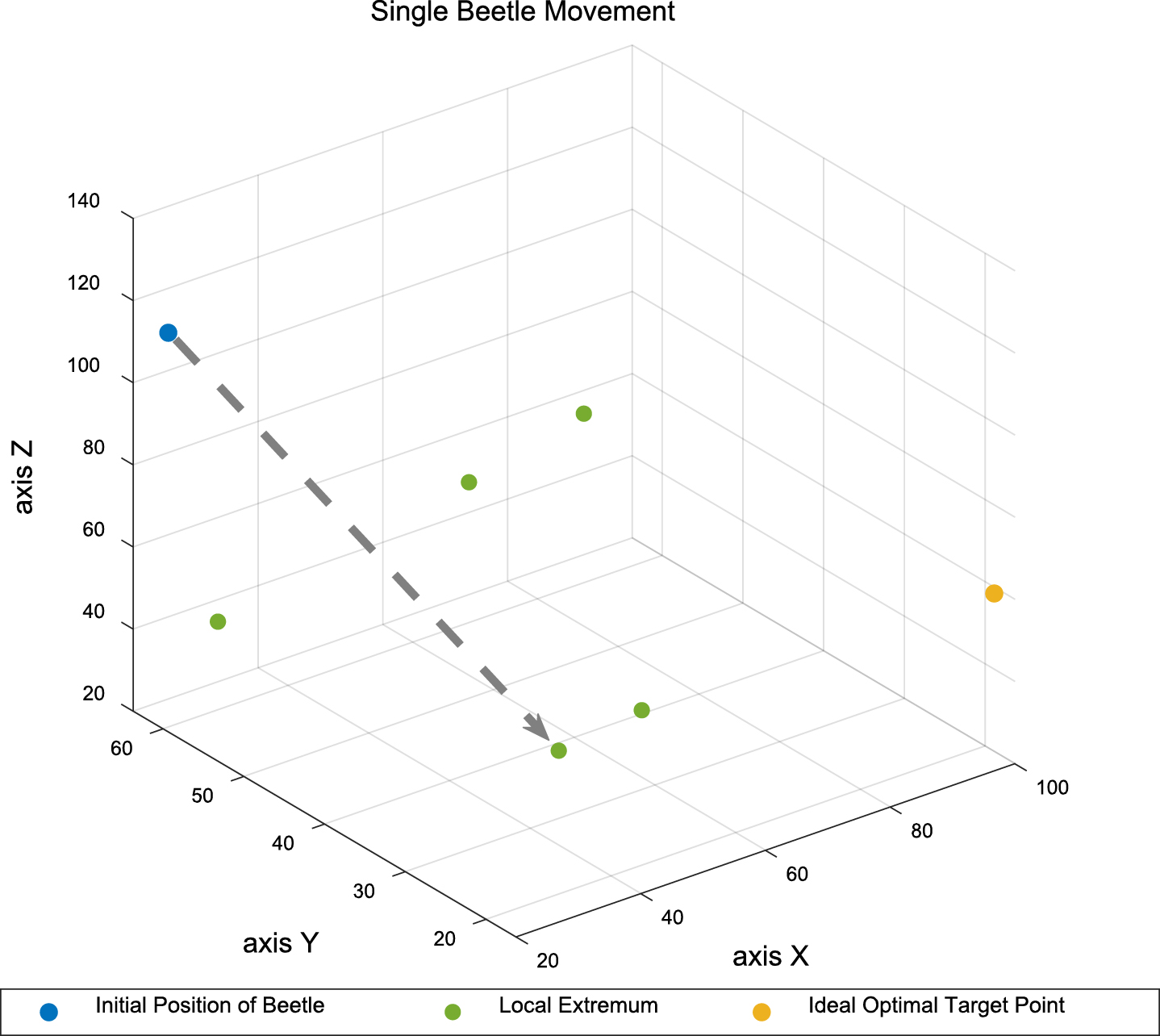
Single beetle movement.

Fig. 5

Beetle swarm movement.

3.2.2 Levy flight strategy with nonlinear sinusoidal disturbance

According to Equation (21) and (22), when a beetle updates its position, it flies in the direction of the well- adapted tentacle in a straight line along with the current step size. Based on this principle, the beetle is very easy to fall into the local extreme value region, resulting in inaccurate results. What’s more, the beetle does not have the ability to jump out of the local extreme value. Therefore, in this paper, we introduced the Levy flight strategy with nonlinear sinusoidal disturbance to simulate the motion behavior of the position update of the beetle swarm. We employ its random walk characteristics to solve the problem of being difficult to change the direction of motion in the search process.

Levy flight strategy is a random walk model that conforms to the Levy distribution [36]. Many insects and birds in nature conform to the Levy distribution model. Most of its trajectory movement shows small step, and occasionally a larger step. Levy flight formula is as follows: $\begin{matrix} L (β) = \frac{μ}{{| ν |}^{- β}}, β = 3 / 2 \end{matrix}$

$σ = \frac{Γ (1 + β) sin (\frac{π β}{2})}{β Γ (\frac{1 + β}{2}) 2^{\frac{β - 1}{2}}}$ (26)

Where, L (β) is the step length of the Levy distribution with the parameter β in the random direction. In this paper, μ and ν all obey the normal distribution, μ ∼ N (0, σ²), ν ∼ N (0, 1), Γ represents the gamma function, 1 < β < 3. in this paper, we let β = 2, the Levy flight motion simulation diagram is as follows:

It can be seen from Fig. 6 that during Levy flight, large jumps occasionally occur, and most of them are in small steps. Meanwhile, the direction of Levy flight strategy changes randomly. In the improved algorithm, Equation (11) is used to replace the position update step in the original BAS:

Fig. 6

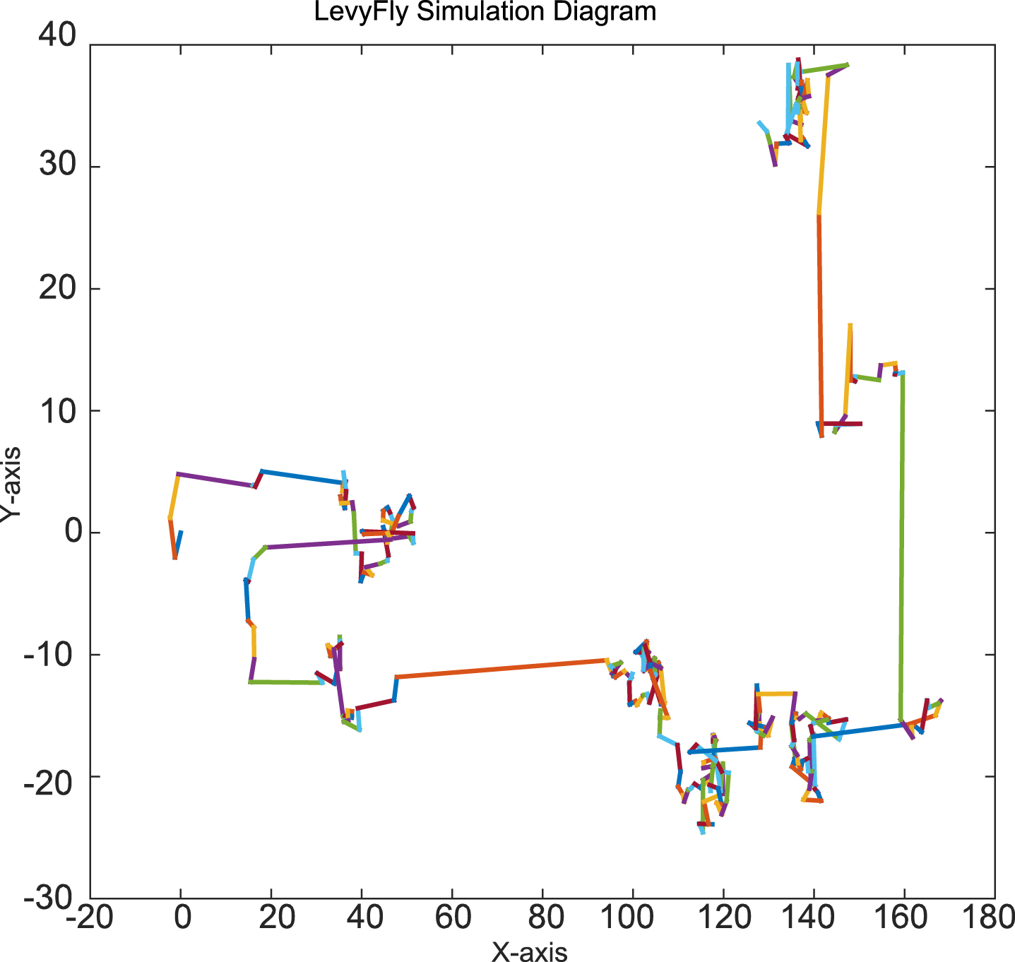
Levy flight motion simulation diagram.

$x_{t + 1} = x_{t} - step * \vec{dir} * sign (f (x_{l}) - f (x_{r})) \otimes L (β)$ (27)

Where, ⊗ represents the vector operation (point-to-point multiplication according to the vector method). The Levy flight strategy is introduced into the positioning of the beetle, which mimics the biological behavior of a beetle exploring the food smell and constantly flying towards the food source. It changes the behavior of a beetle flying along the antennae direction in the original BAS algorithm, which is in favor of enhancing the ability of global exploration and enabling the beetle to jump out of the search domain of the local extreme value.

Because BAS algorithm is prone to search stagnation and premature convergence, Shen et al. [37] proposed a method to change the forward direction of a beetle by the disturbance generated by rand random number to jump out of local optimization. In this paper, the random number disturbance generated by nonlinear sinusoidal disturbance is used to increase the ability to jump out of premature convergence. We add a disturbance term to Equation (22) and adjust the peak value of the function by using the number of iterations and the waveform of the sine function, so that the function has a large fluctuation in the early stage of iteration or when the fitness value is large, which helps BAS algorithm jump out of premature convergence. In the late stage of iteration or when the fitness value is small, it has a small fluctuation, which helps to optimize the feasible solution and avoid stagnation. The adjustment formula of disturbance term is shown in Equation (28):

$r = rand * ({sin}^{ω} (\frac{π}{2} * \frac{t}{t_{max}}) + cos (\frac{π}{2} * \frac{t}{t_{max}}) - 1)$ (28)

In Equation (28), rand represents a random number that obeys Gaussian normal distribution; t is the number of iterations; ω represents the constant value of the t–thiteration. According to Equation (28), we can see that the value of ω affects the peak value of the disturbance factor. In order to explore the influence of the value of ω on the peak value of nonlinear sinusoidal disturbance, we select different values of ω for simulation. It can be concluded from Fig. 7 that the value of ω is different, and the amplitude position of the disturbance factor changes accordingly. When ω = 2, the amplitude is large and the coverage is wide, which helps the algorithm to jump out of the local optimum in the later stage; when ω = 2.5 and ω = 3, the amplitude range of the disturbance factor is not as large as when ω = 2, so we takes ω = 2.

Fig. 7

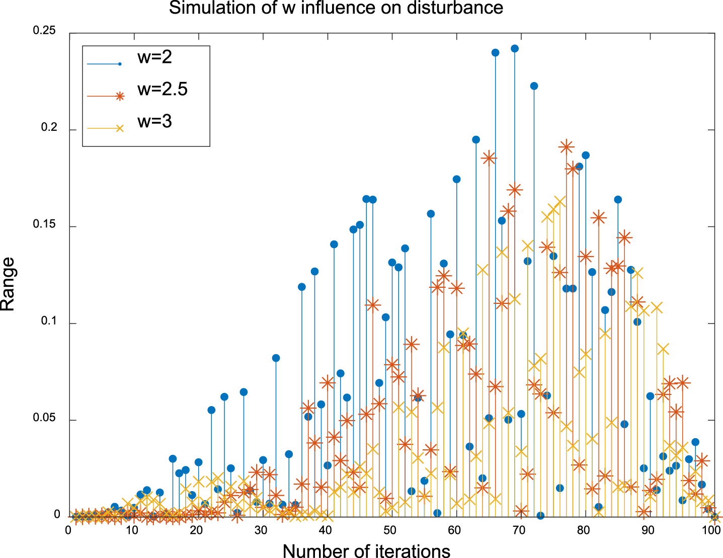
The influence of the value of ωon disturbance.

According to the improvements discussed, the beetle for updating the position shown in Equation (29):

$\begin{matrix} x_{t + 1} = & x_{t} - step * \vec{dir} * sign (f (x_{l}) \\ - f (x_{r})) \otimes L (β) + r \end{matrix}$ (29)

3.2.3 Integrated with artificial bee colony algorithm neighborhood search

The ABC algorithm is a swarm intelligence algorithm [38]. The algorithm includes three roles: hire bee, follow bee, and scout bee. In the stage of hire bees and follow bees, they search for nectar sources near their domains, calculate fitness values, and judge the fitness function values of the new and old nectar sources to make a choice:

$f_{new} = f_{i, D} + rand * (f_{i, D} - f_{k, D})$ (30)

${fitness}_{i} = {\begin{matrix} \frac{1}{(1 + {value}_{i})} {value}_{i} ⩾ 0 \\ 1 + abs ({value}_{i}) {value}_{i} < 0 \end{matrix}$ (31)

Where, f_new is the formula for bees to search for new nectar sources nearby, f_i,D corresponds to the i–th nectar source in D dimension, rand takes a random number in (0, 1), fitness is the fitness function, value_iis the objective function of the optimization problem to be sought.

Combining with the characteristics of hire bees and follow bees searching near the field, after each location update of beetle, let it choose a new location near the neighborhood to replace the current location, judge the fitness of the location, and decide whether to stay or discard. Then, continue to search for a location with better fitness and update. The principle of bees searching near the nectar source area in the ABC algorithm is introduced into the BAS algorithm, which can enhance the diversity of the local search results of the population, overcome the problem that a beetle cannot jump out of the local optimum when it falls into the partial optimal solution. Meanwhile, the introduction of the search within the neighborhood can be used as a basis for judging whether the beetle has entered the target range and changing the update of the beetle’s movement position.

4 Benchmark function test and algorithm flow

In order to test the performance of improved algorithm, we use the benchmark function to evaluate the performance of IBSO algorithm and compare the experimental results with the other five algorithms. Then we describe the flow chart of the IBSO algorithm for solving the path planning problem to show the execution process of the algorithm more clearly. The computational complexity of the algorithm is analyzed by pseudo code.

4.1 Benchmark function test

We test the improved algorithm with 10 benchmark functions. The relevant contents of the benchmark function are shown in Table 1. We use the MATLAB R2018 as the simulation software in the experiment.

Table 1
Relevant parameters of standard test function

Benchmark Test Function Search Interval f _min

Sphere $f_{1} (x) = \sum_{i = 1}^{d} x_{i}^{2}$ [–5.12,5.12] 0

Griewank $f_{2} (x) = \sum_{i = 1}^{d} \frac{x_{i}^{2}}{4000} - \prod_{i = 1}^{d} cos (\frac{x_{i}}{\sqrt{i}}) + 1$ [–600,600] 0

Rotated Hyper-Ellipsoid $f_{3} (x) = \sum_{i = 1}^{N} \sum_{j = 1}^{i} x_{j}^{2}$ [–65.536,65.536] 0

Sum Squares $f_{4} (x) = \sum_{i = 1}^{d} i * x_{j}^{2}$ [–10,10] 0

Drop-Wave $f_{5} (x) = - \frac{1 + cos (12 \sqrt{x_{1}^{2} + x_{2}^{2}})}{0.5 (x_{1}^{2} + x_{2}^{2}) + 2}$ [–5.12,5.12] –1

Matyas $f_{6} (x) = 0.26 (x_{1}^{2} + x_{2}^{2}) - 0.48 x_{1} x_{2}$ [–10,10] 0

Schaffer n.2 $f_{7} (x) = 0.5 + \frac{{sin}^{2} (x_{1}^{2} - x_{2}^{2}) - 0.5}{[1 + 0.001 (x_{1}^{2} + x_{2}^{2})]^{2}}$ [–100,100] 0

sum of Different Powers $f_{8} (x) = \sum_{i = 1}^{d} {| x_{i} |}^{i + 1}$ [–1,1] 0

Three-Hump Camel $f_{9} (x) = 2 x_{1}^{2} - 1.05 x_{1}^{4} + \frac{x_{1}^{6}}{6} + x_{1} x_{2} + x_{2}^{2}$ [–5,5] 0

Rastrigin $f_{10} (x) = 10 d + \sum_{i = 1}^{d} [x_{i}^{2} - 10 cos (2 π x_{i})]$ [–5.12,5.12] 0

Benchmark Test Function	Search Interval	f _min
Sphere	$f_{1} (x) = \sum_{i = 1}^{d} x_{i}^{2}$	[–5.12,5.12]	0
Griewank	$f_{2} (x) = \sum_{i = 1}^{d} \frac{x_{i}^{2}}{4000} - \prod_{i = 1}^{d} cos (\frac{x_{i}}{\sqrt{i}}) + 1$	[–600,600]	0
Rotated Hyper-Ellipsoid	$f_{3} (x) = \sum_{i = 1}^{N} \sum_{j = 1}^{i} x_{j}^{2}$	[–65.536,65.536]	0
Sum Squares	$f_{4} (x) = \sum_{i = 1}^{d} i * x_{j}^{2}$	[–10,10]	0
Drop-Wave	$f_{5} (x) = - \frac{1 + cos (12 \sqrt{x_{1}^{2} + x_{2}^{2}})}{0.5 (x_{1}^{2} + x_{2}^{2}) + 2}$	[–5.12,5.12]	–1
Matyas	$f_{6} (x) = 0.26 (x_{1}^{2} + x_{2}^{2}) - 0.48 x_{1} x_{2}$	[–10,10]	0
Schaffer n.2	$f_{7} (x) = 0.5 + \frac{{sin}^{2} (x_{1}^{2} - x_{2}^{2}) - 0.5}{[1 + 0.001 (x_{1}^{2} + x_{2}^{2})]^{2}}$	[–100,100]	0
sum of Different Powers	$f_{8} (x) = \sum_{i = 1}^{d} {\| x_{i} \|}^{i + 1}$	[–1,1]	0
Three-Hump Camel	$f_{9} (x) = 2 x_{1}^{2} - 1.05 x_{1}^{4} + \frac{x_{1}^{6}}{6} + x_{1} x_{2} + x_{2}^{2}$	[–5,5]	0
Rastrigin	$f_{10} (x) = 10 d + \sum_{i = 1}^{d} [x_{i}^{2} - 10 cos (2 π x_{i})]$	[–5.12,5.12]	0

4.1.1 Benchmark function parameter setting

In order to verify the excellent performance of IBSO algorithm. We choose several typical heuristic algorithms and IBSO algorithm for comparative experiments. It includes PSO [39], the original BAS, sooty tern optimization algorithm (STOA) [40], ant lion optimizer (ALO) [41] and artificial bee colony algorithm. To ensuring the fairness of the comparison algorithm and obtain satisfactory results. We set the maximum number of iterations for each algorithm to be 200. The number of search population of each algorithm is 100, and the spatial dimension is 30. Table 2 provides the main parameter settings of the six comparison algorithms.

Table 2
The main parameter settings of the six algorithms

Algorithm Parameter values

PSO Learning factors c1 = c2 = 2; Inertia weight ω = 0.7;

BAS Decrement factor eta = 0.95; step = 1; c = 5;

STOA Control variable c_f = 2; Random variable C_B ∈ [0, 0.5]; u = v = 1;

ALO r_rand ∈ [0, 1]; ω = 2, 3, . . . , 6

ABC Nectar source 50;

IBSO eta = 0.95; step = 1;c = 5; β = 2, ω = 2

Algorithm	Parameter values
PSO	Learning factors c1 = c2 = 2; Inertia weight ω = 0.7;
BAS	Decrement factor eta = 0.95; step = 1; c = 5;
STOA	Control variable c_f = 2; Random variable C_B ∈ [0, 0.5]; u = v = 1;
ALO	r_rand ∈ [0, 1]; ω = 2, 3, . . . , 6
ABC	Nectar source 50;
IBSO	eta = 0.95; step = 1;c = 5; β = 2, ω = 2

4.1.2 Experimental result

We run each algorithm independently for 20 times, and count the average, optimal and worst value of the six algorithms. In the Table 3, Best, Worst and Mean represent the optimal value, worst value and average value. We rank the average solution values obtained by different algorithms according to the quality of the results. Table 3 shows the results of the test results. From the optimal value, worst value, average value and the ranking of the experimental results, we can see the optimization performance of IBSO algorithm.

Table 3
Experimental results of 6 algorithms

Algorithm

Functions Result PSO BAS STOA ALO ABC IBSO

f ₁ Best 3.441E-09 5.038E-06 1.069E-21 7.131E-15 1.377E-23 0

Worst 1.531E-07 1.752E-05 4.253E-17 3.814E-13 4.823E-22 1.050E-159

Mean 2.173E-08 7.177E-06 5.419E-20 5.228E-14 5.898E-23 3.776E-239

Rank 5 6 3 4 2 1

f ₂ Best 0.0074 1.723E-06 0.0078 0.0823 0.0614 0

Worst 0.0298 1.110E-05 0.0366 0.2904 0.1283 0

Mean 0.0193 5.348E-06 0.0188 0.1133 0.1093 0

Rank 4 2 5 3 6 1

f ₃ Best 1.794E-07 1.030E-07 7.956E-19 3.225E-12 1.002E-20 0

Worst 9.552E-05 2.088E-05 1.176E-16 5.825E-10 8.127E-20 2.346E-130

Mean 5.682E-06 1.844E-06 5.738E-18 9.322E-11 4.691E-20 1.494E-172

Rank 6 5 3 4 2 1

f ₄ Best 1.528E-09 9.206E-07 7.632E-23 6.613E-13 1.224E-22 1.667E-304

Worst 9.552E-07 1.845E-05 7.816E-20 1.989E-11 9.340E-22 4.171E-101

Mean 1.563E-08 4.960E-06 1.802E-22 2.360E-12 4.461E-22 4.249E-284

Rank 5 6 2 4 3 1

f ₅ Best –1 –0.9323 –1 –1 –1 –1

Worst –0.9962 –0.5747 –0.9362 –0.9362 –1 –1

Mean –0.9999 –0.8247 –0.9845 –0.9845 –1 –1

Rank 1 6 1 1 1 1

f ₆ Best 9.524E-13 5.087E-13 1.020E-23 6.963E-16 1.065E-27 1.654E-319

Worst 1.785E-10 5.504E-12 7.573E-21 4.134E-14 1.463E-24 1.299E-151

Mean 2.602E-11 4.462E-12 1.444E-21 8.992E-15 3.069E-25 3.039E-267

Rank 6 5 3 4 2 1

f ₇ Best 3.145E-09 1.249E-09 0 1.359E-15 0 0

Worst 1.379E-08 6.684E-03 0 2.196E-13 0 0

Mean 9.342E-09 7.334E-04 0 1.596E-14 0 0

Rank 6 5 1 4 1 1

f ₈ Best 1.367E-13 2.024E-06 5.754E-32 3.031E-12 1.748E-35 0

Worst 6.552E-09 9.189E-05 5.102E-26 9.318E-09 1.560E-34 6.578E-150

Mean 7.793E-10 3.576E-05 5.608E-27 2.169E-09 6.984E-35 6.696E-152

Rank 4 6 3 5 2 1

f ₉ Best 1.893E-13 2.080E-12 9.720E-32 3.404E-15 2.346E-55 6.489E-191

Worst 9.383E-09 2.983E-03 1.385E-27 1.968E-13 2.687E-52 7.950E-76

Mean 1.061E-09 3.351E-04 2.824E-28 6.063E-14 4.412E-53 7.954E-77

Rank 5 6 3 4 2 1

f ₁₀ Best 4.151E-07 0.9980 7.105E-15 1.9899 0.8427 0

Worst 1.253E-04 7.5814 2.0829 4.9748 2.4303 0

Mean 2.680E-05 3.8263 0.8019 3.2547 1.6271 0

Rank 3 5 2 6 4 1

		Algorithm
f ₁	Best	3.441E-09	5.038E-06	1.069E-21	7.131E-15	1.377E-23	0
	Worst	1.531E-07	1.752E-05	4.253E-17	3.814E-13	4.823E-22	1.050E-159
	Mean	2.173E-08	7.177E-06	5.419E-20	5.228E-14	5.898E-23	3.776E-239
	Rank	5	6	3	4	2	1
f ₂	Best	0.0074	1.723E-06	0.0078	0.0823	0.0614	0
	Worst	0.0298	1.110E-05	0.0366	0.2904	0.1283	0
	Mean	0.0193	5.348E-06	0.0188	0.1133	0.1093	0
	Rank	4	2	5	3	6	1
f ₃	Best	1.794E-07	1.030E-07	7.956E-19	3.225E-12	1.002E-20	0
	Worst	9.552E-05	2.088E-05	1.176E-16	5.825E-10	8.127E-20	2.346E-130
	Mean	5.682E-06	1.844E-06	5.738E-18	9.322E-11	4.691E-20	1.494E-172
	Rank	6	5	3	4	2	1
f ₄	Best	1.528E-09	9.206E-07	7.632E-23	6.613E-13	1.224E-22	1.667E-304
	Worst	9.552E-07	1.845E-05	7.816E-20	1.989E-11	9.340E-22	4.171E-101
	Mean	1.563E-08	4.960E-06	1.802E-22	2.360E-12	4.461E-22	4.249E-284
	Rank	5	6	2	4	3	1
f ₅	Best	–1	–0.9323	–1	–1	–1	–1
	Worst	–0.9962	–0.5747	–0.9362	–0.9362	–1	–1
	Mean	–0.9999	–0.8247	–0.9845	–0.9845	–1	–1
	Rank	1	6	1	1	1	1
f ₆	Best	9.524E-13	5.087E-13	1.020E-23	6.963E-16	1.065E-27	1.654E-319
	Worst	1.785E-10	5.504E-12	7.573E-21	4.134E-14	1.463E-24	1.299E-151
	Mean	2.602E-11	4.462E-12	1.444E-21	8.992E-15	3.069E-25	3.039E-267
	Rank	6	5	3	4	2	1
f ₇	Best	3.145E-09	1.249E-09	0	1.359E-15	0	0
	Worst	1.379E-08	6.684E-03	0	2.196E-13	0	0
	Mean	9.342E-09	7.334E-04	0	1.596E-14	0	0
	Rank	6	5	1	4	1	1
f ₈	Best	1.367E-13	2.024E-06	5.754E-32	3.031E-12	1.748E-35	0
	Worst	6.552E-09	9.189E-05	5.102E-26	9.318E-09	1.560E-34	6.578E-150
	Mean	7.793E-10	3.576E-05	5.608E-27	2.169E-09	6.984E-35	6.696E-152
	Rank	4	6	3	5	2	1
f ₉	Best	1.893E-13	2.080E-12	9.720E-32	3.404E-15	2.346E-55	6.489E-191
	Worst	9.383E-09	2.983E-03	1.385E-27	1.968E-13	2.687E-52	7.950E-76
	Mean	1.061E-09	3.351E-04	2.824E-28	6.063E-14	4.412E-53	7.954E-77
	Rank	5	6	3	4	2	1
f ₁₀	Best	4.151E-07	0.9980	7.105E-15	1.9899	0.8427	0
	Worst	1.253E-04	7.5814	2.0829	4.9748	2.4303	0
	Mean	2.680E-05	3.8263	0.8019	3.2547	1.6271	0
	Rank	3	5	2	6	4	1

According to the data in Table 3, the 10 benchmark functions are run independently for 20 times, and the IBSO algorithm can find the optimal value for the test functions f₂,f₅, f₇ and f₁₀. In the results of benchmark test functions f₁, f₃ and f₈, the optimal solution can be achieved, and the average solution value shows a considerable improvement in the accuracy of the solution compared with the other five algorithms. Although the results of benchmark functions f₄, f₆ and f₉ do not reach the optimal solution, its solution accuracy is considerably improved compared with the other algorithms, and the solution result is better than that of the comparison algorithm. In order to more intuitively show the excellent performance of the IBSO algorithm, Fig. 8 are the iterative convergence diagrams of the six algorithms. In order to more clearly show the convergence effect of the algorithm, some functions use the logarithmic function representation for the fitness value.

Fig. 8

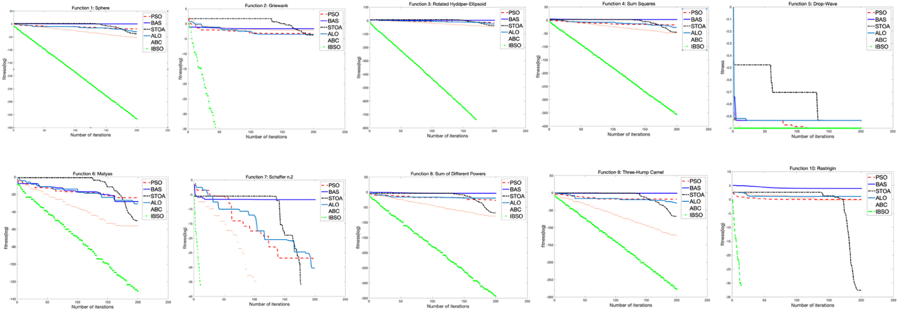
f₁-f₁₀ Iterative convergence graph.

According to the iterative convergence diagrams of 6 optimization algorithms to solve 10 benchmark test functions, it can be seen that the test functions f₂,f₅,f₇ and f₁₀ can be solved to the optimal solution when the iteration is less than 50 times. Among other benchmark functions, the IBSO algorithm shows better solution accuracy and faster convergence speed, which is due to the fast convergence characteristics of the beetle algorithm. In addition, we study and analyse the distribution characteristics of the benchmark functions solved by IBSO and comparison algorithms in 20 independent experiments. As shown in Fig. 9, the box diagram analysis is shown. We proposed IBSO performs well in most functions compared to other competitors. The median, maximum and minimum values of the objective functions obtained by IBSO are almost the same as the optimal solutions, especially for f₂, f₅, f₇ and f₁₀. In the box diagram, f₁, f₃, f₄, f₆, f₈ and f₉, we can see that there is a gap between the maximum and minimum solution ranges of IBSO algorithm, but according to the statistical data in Table 3, IBSO solution values are superior to other comparison algorithms when the solution accuracy changes.

Fig. 9

Box diagram analysis for benchmark f₁-f₁₀.

From the analysis of iterative convergence graph and box graph of benchmark functions, it is obvious that the IBSO algorithm we proposed has shown comparable better computational performance, which further proves the validity of IBSO algorithm.

Therefore, IBSO shows the potential to be a better optimizer for solving global optimization problems, particularly, it has good computational performance in solving complex nonlinear problems. It in turn provides a feasible basis for the IBSO algorithm to solve some complex nonlinear calculation modelling in the path planning problem.

4.2 Algorithm flow

The implementation flow chart of the IBSO algorithm in path planning problem is shown in Fig. 10:

Fig. 10

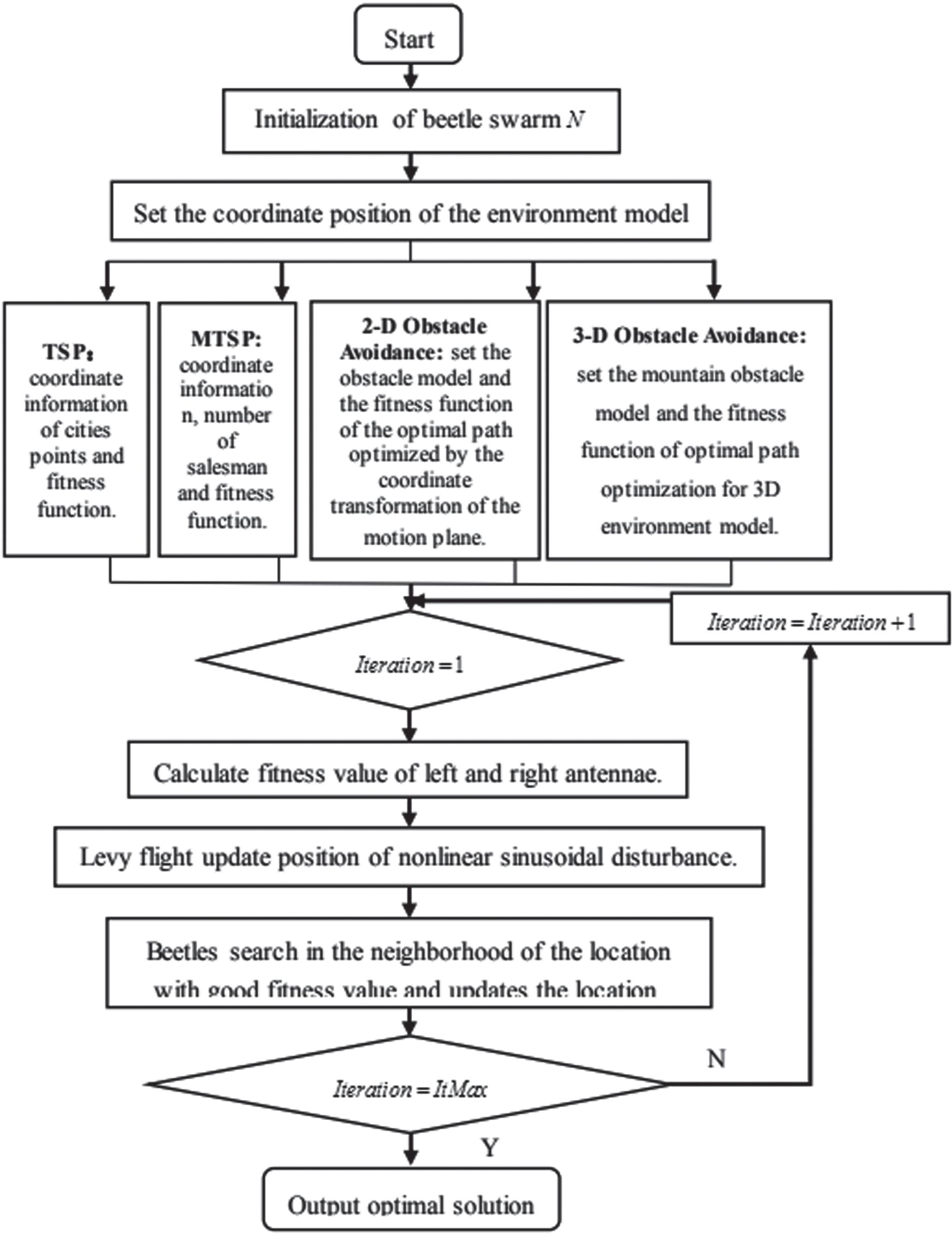
Flow chart of IBSO for path planning.

The pseudo code of the above model is presented in Algorithm 1.

The number of executions of basic operations when an algorithm solves a problem is defined as the time complexity of the algorithm. The original BAS algorithm is simple in principle and fast in execution. The time complexity can be expressed as T (N) = O (DIter_i). Among them, D represents the spatial dimension of the problem to be solved, and Iter_i represents the number of iterations of the algorithm to solve the problem, so the time complexity of the BAS algorithm is O (1). The spatial dimension of the IBSO algorithm proposed in this paper is still D, and the number of iterations is still T_i. After a single beetle transformed into beetle swarm, the population number becomes N_s, and in each iteration process, it is converted from a beetle search to a population number N_s for solution. Optimization increases the computational complexity of the algorithm execution, and increases the solution time. N_s has a greater impact on the computational complexity of the enhanced algorithm, but the introduced Levy flight strategy for vector operations and step disturbance factor r are both within a small range. The numerical value has little effect on the computational complexity of the algorithm. The idea of neighborhood search combined with artificial bee colony algorithm is to reselect points near the current optimal location for fitness calculation and compare it with the current best point. Therefore, the increased calculation process is O (Iter_iN_s). Therefore, the time complexity of the enhanced algorithm can be roughly expressed as T (N) = O (DIter_iN_s + Iter_iN_s + r ⊗ L (β)), that is, O (N). Therefore, the computational complexity of the IBSO algorithm is slightly larger than that of the BAS algorithm.

5 Application of IBSO algorithm in path planning

The IBSO algorithm achieves ideal performance results in the benchmark function. Next, it is tested whether the IBSO algorithm still has good solution performance in the path planning optimization problems. In this paper, we choose two kinds of common path planning problems: the ergodic optimal path problem in the discrete domain and the global path planning problem in the continuous domain. The experimental contents including TSP, MTSP, and obstacle avoidance problem of simulated robots in 2D plane and 3D environment. According to different solving problems, we carry out modeling and analysis, and use the proposed IBSO algorithm to solve them.

In this paper, without considering other real-time factors, our modeling and simulation are tested in an idealized static environment model. We regard UAV as a mass point.

5.1 Experimental process analysis

The specific steps of using the proposed IBSO algorithm in path planning problem are as follows:

Analyze and model the path planning problem to determine the optimal objective function.

Improve the traditional beetle antennae search algorithm.

Use the improved IBSO algorithm to optimize different path planning problems.

In the IBSO algorithm, the location information of the beetle swarm is expressed as the optimal path distance length. The shortest cumulative length of the path line is used as the value of the fitness function for the optimization algorithm. Each model is run 20 times independently. We take the average as the comparison data.

The detailed parameter settings of the test experiment are shown in Table 4:

Table 4
Experimental parameter setting

Parameter Represent Value

popsize Beetle population 50

D Spatial dimension 20

max iter Maximum number of iterations 100

d Distance between two antennae 1

step Beetle step size 1

eta Beetle step size decreasing factor 0.95

ω Constant value of t–th iteration 2

β Distribution with parameter β 2

Parameter	Represent	Value
popsize	Beetle population	50
D	Spatial dimension	20
max iter	Maximum number of iterations	100
d	Distance between two antennae	1
step	Beetle step size	1
eta	Beetle step size decreasing factor	0.95
ω	Constant value of t–th iteration	2
β	Distribution with parameter β	2

5.2 Test case and analysis of ergodic optimal path problem in discrete domain

5.2.1 Case A: optimization of the traveling salesman problem

There are many optimization algorithms for solving TSP. The PSO has the advantages of fast search, easy implementation, and simple parameter setting. It is suitable for solving combinatorial optimization problems [42]. The ant colony optimization (ACO) algorithm selects the next path based on probability, and the ants will secrete pheromone substances on the path when they travel, avoiding the path that has been traveled, and select the next city according to the probability calculated by the heuristic factor, so that the ACO algorithm has great advantages for solving the TSP [43]. In order to verify the effectiveness of the improved algorithm in this paper, we use the above two algorithms to solve TSP as the comparison of the algorithm in this paper, and cite the experimental results of the literature [44 –46] for comparison. The TSPLIB database [47] is used to test the simulation, the test platform is MATLAB R2018a. The data instance is continuously tested for 20 times, and the optimal value and average value are recorded. The experimental results are shown in Table 5. Table 5 Simulation results of the improved algorithm

Table 5
Simulation results of the improved algorithm

TSP Case TSPLIB Optimal solution Algorithm Average value Optimal value Relative error

(RE/%)

Bayg29 (29 cities) 9.07e+03 PSO 1.0904E+04 1.0143E+04 21.4

ACO 9.2721E+03 9.2294E+03 2.3

MFPOA [46] 1.4266E+04 1.2467E+04 57.3

MQHOA [46] 1.3786E+04 1.5697E+04 52

IBSO 9.0770e+03 9.0741e+03 0.03

Burma14 (14 cities) 30.8785 PSO 31.4035 31.2089 1.7

ACO 31.2674 31.2269 1.4

Reference [44] 31 31 0.04

CSO [45] – 31 –

FFA [45] – 31 –

MFPOA [46] 32.53 30.87 5.3

MQHOA [46] 31.65 34.47 2.5

IBSO 30.8785 30.8785 0

Dantzig42(42 cities) Current optimal: 699 PSO 1.0515E+03 9.3799E+02 50.5

ACO 7.8043E+02 7.4124E+02 8.7

Reference [44] – 689 –

CSO [45] – 689 –

FFA [45] – 699 –

IBSO 7.0191E+02 6.8676E+02 0.42

TSP Case	TSPLIB Optimal solution	Algorithm	Average value	Optimal value	Relative error
Bayg29 (29 cities)	9.07e+03	PSO	1.0904E+04	1.0143E+04	21.4
		ACO	9.2721E+03	9.2294E+03	2.3
		MFPOA [46]	1.4266E+04	1.2467E+04	57.3
		MQHOA [46]	1.3786E+04	1.5697E+04	52
		IBSO	9.0770e+03	9.0741e+03	0.03
Burma14 (14 cities)	30.8785	PSO	31.4035	31.2089	1.7
		ACO	31.2674	31.2269	1.4
		Reference [44]	31	31	0.04

		CSO [45]	–	31	–
		FFA [45]	–	31	–
		MFPOA [46]	32.53	30.87	5.3
		MQHOA [46]	31.65	34.47	2.5
		IBSO	30.8785	30.8785	0
Dantzig42(42 cities)	Current optimal: 699	PSO	1.0515E+03	9.3799E+02	50.5
		ACO	7.8043E+02	7.4124E+02	8.7
		Reference [44]	–	689	–
		CSO [45]	–	689	–
		FFA [45]	–	699	–
		IBSO	7.0191E+02	6.8676E+02	0.42

It can be seen from Table 5 that the IBSO algorithm has a great improvement in the solution accuracy. Among them, the test set burma14 can be solved to the optimal value, and the relative error value of the test set bayg29 is approximately 0. The theoretical optimal solution can be obtained in 20 simulation tests. The relative error of IBSO algorithm is significantly lower than that of other comparison algorithms. In the test set dantzig42, the relative errors of the PSO and ACO algorithms are as high as 50.5% and 8.7%, while the solution values of the IBSO algorithm and the reference [44, 45] are further improved, but the results of the IBSO algorithm are better. The simulation comparison of the above three test sets shows that the IBSO is more accurate in solving TSP. Figure 11 is the optimal path diagram of the solution of the three test sets by the IBSO algorithm.

Fig. 11

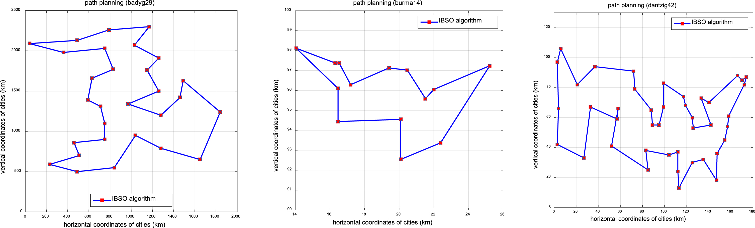
Optimal path of three test set cases.

The following is the TSP case simulation time of the three test set cases as shown in Table 6 and the algorithm convergence comparison graph as shown in Fig. 12.

Table 6

Simulation time comparison of three algorithms

TSP Case	Algorithm	Simulation Time/s	TSP Case	Algorithm	Simulation Time/s
Bayg29	PSO	2.2367	Burma14	PSO	1.4903
	ACO	7.6613		ACO	2.9014
	GA [46]	18.51		GA [46]	16.17
	AS [46]	2.09		AS [46]	1.99
	HPSO [46]	40.57		HPSO [46]	33.05
	MFPOA-DS [46]	7.03		MFPOA-DS [46]	7.07
	IBSO	1.9579		IBSO	1.4801
TSP Case		Algorithm		Simulation Time/s
Dantzig42		PSO		2.8712
		ACO		14.3919
		IBSO		2.6113

Fig. 12

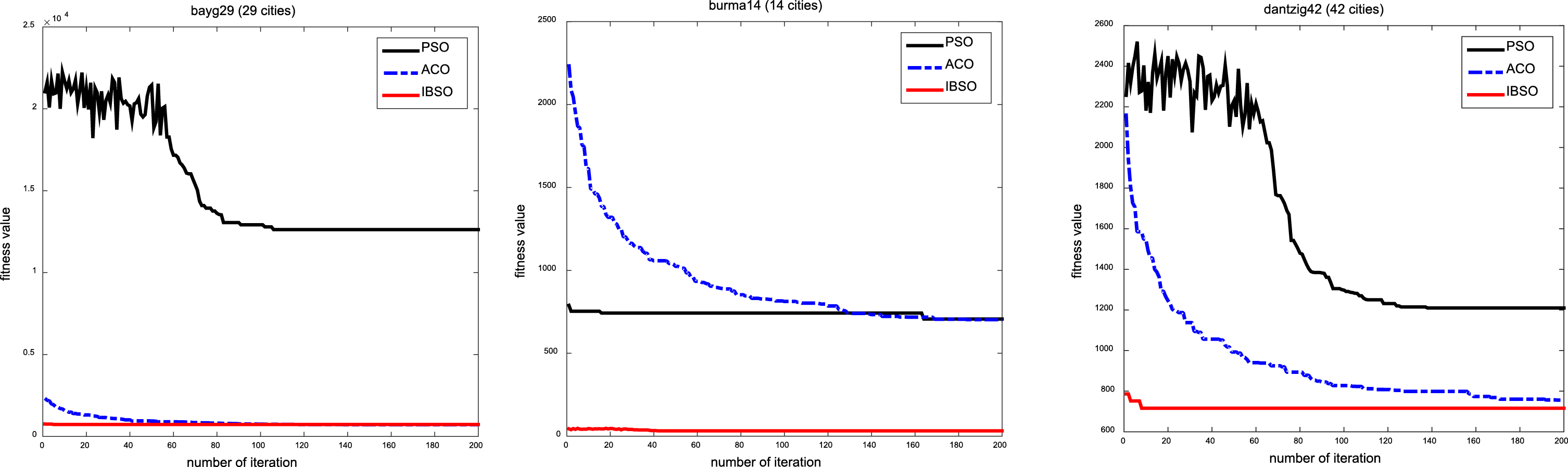
Iterative curve of three test set cases.

It can be seen from Table 6 that the ACO algorithm has the longest running time, which is about 2–7 times than the IBSO algorithm. The running time of the PSO algorithm and the IBSO algorithm is shorter, but the IBSO algorithm we proposed is 0.3 s shorter on average than the PSO algorithm. Among the comparison algorithms in reference [46], the simulation time of AS algorithm is the shortest, but it is also higher than that of IBSO algorithm. Comparing the iterative convergence curves of the three algorithms, case bayg29, the IBSO algorithm finds the optimal solution after about 30 iterations, the PSO and ACO find the optimal solution after 120 and 80 iterations, respectively. Case burma14, the number of cities is small, and the solution results of the three algorithms are all close to the optimal value. It can be seen from the iterative graph that the convergence effect of the IBSO algorithm is worse than that of the ACO algorithm in the early iteration. This is because the IBSO algorithm needs to determine the position and orientation of the beetle, and once the target orientation is determined, the solution can be quickly converged. In addition, in this case, the IBSO algorithm can solve the optimal solution value, while the PSO and ACO algorithms do not solve the optimal solution value. In the case of dantzig42, the IBSO algorithm finds the optimum after about 50 iterations, while the PSO algorithm falls into a local extremum at about 110 iterations, indicating that the PSO algorithm is not suitable for solving the multi-city TSP problem. The ACO algorithm has not yet found the optimal solution after reaching the maximum number of iterations. It can be seen from the above analysis that the convergence speed of our proposed IBSO algorithm is faster than other algorithms, the running time is shorter, and the solution performance is better.

5.2.2 Case B: MTSP optimization

In the previous section, we tested the IBSO algorithm with the classical TSP problem in the path planning problem. In this section, we applied the IBSO algorithm to the extended TSP problem: the solution of MTSP. Similarly, referring to the TSPLIB test data set. The data case is continuously tested for 20 simulations, and the maximum number of iterations is 200. The number of travel agents is 5. The optimal value was recorded, and the experimental results are shown in Table 7.

Table 7
Simulation results of the improved algorithm

TSP Case TSPLIB Optimal value Algorithm Optimal value

Burma14 3323 IBSO 3323

Bayg29 1610 IBSO 1610

Hk48 11461 FA [48] 11482

IBSO 11465.1105

Eil51 426 FA [48] 428.739

IWO [49] 1465.2615

PGA [49] 610.0616

PSO [49] 1079.2563

IPGA [49] 428.981

MFFA [50] 436.16

PSOPS [51] 768.181

IBSO 427.4014

St70 675 FA [48] 687.75

PGA [49] 1055.4422

IPGA [49] 677.1945

PSO [49] 2670.2450

Reference [52] 689.4

IBSO 676.5802

KorA100 21282 IPGA [49] 21482.27

PSOPS [51] 84224.503

Reference [52] 21625.7

Reference [53] 21352

IBSO 21287.3316

TSP Case	TSPLIB Optimal value	Algorithm	Optimal value
Burma14	3323	IBSO	3323
Bayg29	1610	IBSO	1610
Hk48	11461	FA [48]	11482
		IBSO	11465.1105
Eil51	426	FA [48]	428.739
		IWO [49]	1465.2615
		PGA [49]	610.0616
		PSO [49]	1079.2563
		IPGA [49]	428.981
		MFFA [50]	436.16
		PSOPS [51]	768.181
		IBSO	427.4014
St70	675	FA [48]	687.75
		PGA [49]	1055.4422
		IPGA [49]	677.1945
		PSO [49]	2670.2450
		Reference [52]	689.4
		IBSO	676.5802
KorA100	21282	IPGA [49]	21482.27
		PSOPS [51]	84224.503
		Reference [52]	21625.7
		Reference [53]	21352
		IBSO	21287.3316

The path diagram of IBSO algorithm to solve MTSP test cases is shown in Fig. 13:

Fig. 13

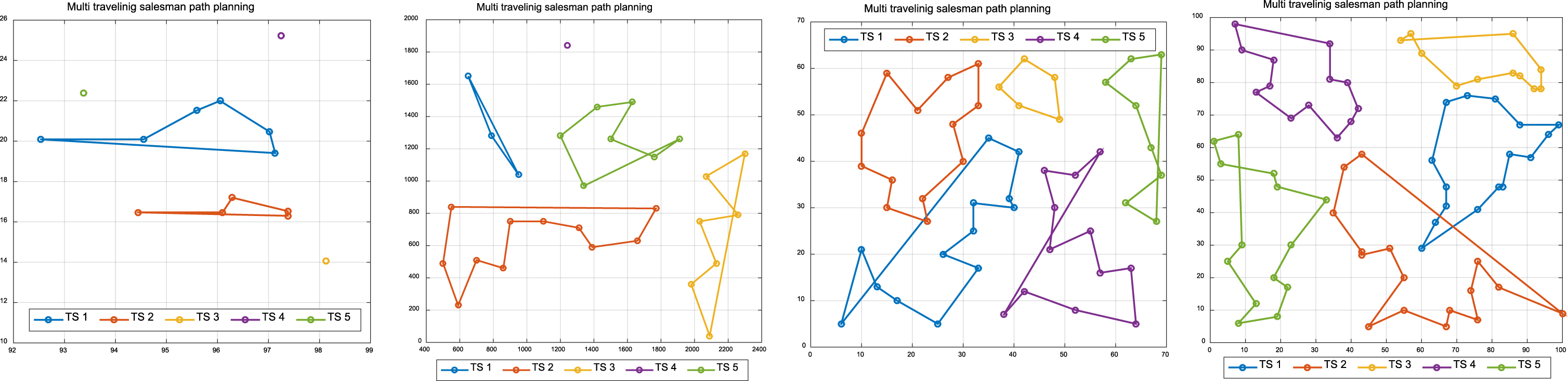
Path planning.

It can be seen from Table 7 that our proposed IBSO also has good computational performance in solving the multi-travelling salesman problem. In Burma14 and Bayg29, which have a small number of cities, IBSO can solve the current optimal solution. With the increase of the number of cities, the calculation degree is complicated. Although the IBSO algorithm cannot solve the current optimal solution, it has a great improvement in the solution results compared with the other algorithms, and is the closest to the current known optimal solution. From Fig. 13, we can see that the IBSO algorithm solves the MTSP case, which can better allocate cities to multiple travelling salesmen. Combining the solution path planning diagram and the solution results, it can be seen that IBSO has better performance in solving the multi-travelling salesman problem.

5.3 Test case and analysis of global path planning problem in continuous domain

5.3.1 Case A: path planning for 2D obstacle avoidance

In this section, we use the proposed IBSO algorithm to shorten the optimization time and provide a new idea for the mobile robot to avoid obstacles in time. The IBSO algorithm can find the current optimal path and obtain a smooth collision-free and smooth obstacle avoidance path. It effectively improves the problem of avoiding obstacles during the real-time movement of the intelligent control robot and increases the safety.

Two cases are simulated in MATLAB environment based on the improved beetle swarm optimization algorithm, and compared with PSO, ABC, improved artificial bee colony algorithm [58], literature [59] TPBSO algorithm are compared to prove the effectiveness of the IBSO algorithm. The initial number of the beetle population is 50, the initial step of the beetle is step = 1, and the distance between two antennae is d = 2. The particle swarm population is 200, and the learning factor is set to 2; the ABC employs 40 bees. The maximum number of iterations of each algorithm It max = 600times, and the search is performed in the spatial dimension D = 30. The simulation results of the five algorithms are as follows.

CASE 1: The layout settings of the threat obstacle and the simulation results are shown in Table 8 and Fig. 14:

Table 8
CASE A: threat obstacle setting

Number of obstacles Obstacle center Obstacle radius Number of obstacles Obstacle center Obstacle radius

1 (350,200) 140 8 (480,110) 90

2 (100,0) 50 9 (40,100) 40

3 (305, –150) 150 10 (470, –50) 30

4 (105,110) 30 11 (300,0) 40

5 (175,110) 25 12 (400,0) 40

6 (245,110) 25 13 (150,50) 40

7 (415,0) 25

Number of obstacles	Obstacle center	Obstacle radius	Number of obstacles	Obstacle center	Obstacle radius
1	(350,200)	140	8	(480,110)	90
2	(100,0)	50	9	(40,100)	40
3	(305, –150)	150	10	(470, –50)	30
4	(105,110)	30	11	(300,0)	40
5	(175,110)	25	12	(400,0)	40
6	(245,110)	25	13	(150,50)	40
7	(415,0)	25

Fig. 14

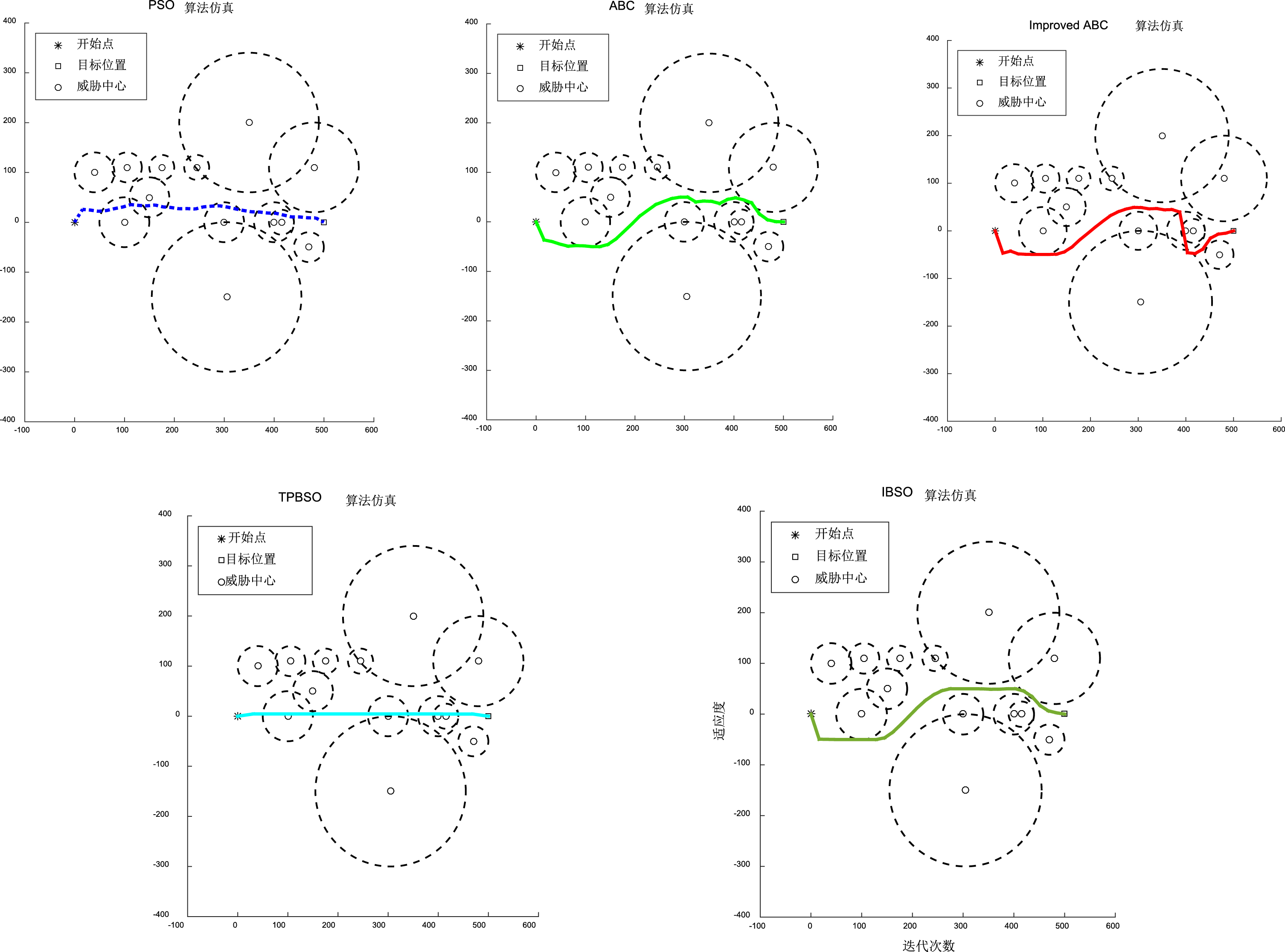
CASE 1 path planning of five algorithms.

It can be seen from the operation images that the PSO algorithm and the TPSBO algorithm did not avoid obstacles in the early stage of the iteration, the ABC algorithm and the improved ABC algorithm have a good optimization effect in the early stage of the iteration, but with the characteristics of the algorithm itself, the convergence rate slows down, and the limitations of the algorithm appear. In the later stage, the small object obstacle is not well avoided, and the optimization process enters the obstacle radius. The IBSO algorithm proposed in this paper avoids obstacles well in the entire iterative optimization process, without touching. Secondly, from the motion trajectory, the PSO algorithm has minor fluctuations and has many inflection points; the motion trajectory of the ABC algorithm and the improved ABC algorithm fluctuates in a small range in the later stage; the motion trajectory of the ABC algorithm is not smooth; the motion trajectory of the IBSO algorithm is smoother than other algorithms, with no inflection points. Tables 9 10 list the comparison of different indicators.

Table 9

Comparison of five algorithms

Algorithm	Running time/s	Iterations	Total path length/m
PSO	3.145337	600	553.0275
ABC	2.196518	600	549.6818
Improved ABC	2.178544	600	556.7467
TPBSO	2.295372	600	556.3782
IBSO	1.307620	600	542.0078

Table 10

Comparison of average data of five algorithms

Algorithm	Average time/s	Average iterations	Average objective function value	Variance
PSO	3.147752	320	3.33531	1.56 × 10^-4
ABC	2.533391	414	2.97428	5.49 × 10^-4
Improved ABC	2.472352	780	2.96391	3.53 × 10^-5
TPBSO	2.455639	430	2.71826	2.33 × 10^-5
IBSO	1.893785	270	2.20497	6.81 × 10^-6

From the analysis of Tables 9 10, it can be seen that under the same number of iterations, the convergence speed of the IBSO algorithm is shortened by at least 0.5 seconds on average. This is precisely due to the rapid optimization and convergence of the BAS algorithm, which enables the intelligent control robot to respond quickly and avoid obstacles when it is about to touch an obstacle. From the perspective of optimal path length, the path lengths measured by the PSO algorithm, the ABC algorithm, the improved ABC algorithm and the TPBSO algorithm from the simulation experiments are all higher than the IBSO algorithm. The results measured by the IBSO algorithm not only smooth the trajectory, but also reduce the path length by nearly 10 meters. The IBSO algorithm proposed in this paper is lower than other algorithms in terms of average objective function mean and index value variance. Therefore, the IBSO algorithm is relatively stable, and the optimization effect and robustness are strong. It can solve the problem of intelligent control robot avoiding obstacles in 2D environment very well.

CASE 2: The layout settings of the threat obstacle and the simulation results are shown in Tables 11 12 and Fig. 15:

Table 11

CASE B: threat obstacle setting

Number of obstacles	Obstacle center	Obstacle radius	Number of obstacles	Obstacle center	Obstacle radius
1	(100, 0)	40	9	(250, –50)	40
2	(200, 0)	40	10	(350, –50)	40
3	(300, 0)	40	11	(0, 40)	20
4	(400, 0)	40	12	(466, 40)	20
5	(150, 50)	40	13	(250, –300)	200
6	(250, 50)	40	14	(250, 300)	200
7	(350, 50)	40	15	(466, –40)	20
8	(150, –50)	40	16	(30, –20)	30

Table 12

Comparison of five algorithms

Algorithm	Running time/s	Iterations	Total path length/m
PSO	4.192242	1000	497.1425
ABC	2.682961	1000	492.2713
Improved ABC	2.732112	1000	554.1501
TPBSO	2.635582	1000	494.3593
IBSO	2.130665	1000	487.0260

Fig. 15

CASE 2 path planning and iterative convergence comparison diagram of five algorithms.

In case 2, the obstacle environment is more complex. According to the simulation operation diagram, both the PSO algorithm and the TPBSO algorithm have many inflection points and pass through obstacles; the improved ABC algorithm crosses obstacles in the early stage of operation, and the simulation effect is poor; The running trajectory of the ABC algorithm and the IBSO algorithm in this paper are similar, but it can be seen from the figure that the running trajectory of IBSO is smoother. It can also be seen from the iterative convergence diagram that the IBSO algorithm in this paper has the best optimization results, which further verifies this paper still has good operating results in the case of more complex obstacle environments, which provides an effective solution to the obstacle avoidance problem of mobile robots in 2D space, and further proves the effectiveness of the IBSO algorithm.

5.3.2 Case B: 3D obstacle avoidance path planning problem

In the previous section, we discussed the path planning scheme for solving the obstacle avoidance problem with the IBSO algorithm in the 2D environment. In this section, we further discuss the path planning scheme for solving the obstacle avoidance problem with the IBSO algorithm in the 3D space. Many researchers have also studied the solution of obstacle avoidance problem in 3D path planning. At present, the mainstream algorithm for solving this kind of problem is based on the improvement of the traditional obstacle avoidance algorithm, such as the improved A* algorithm [56] and the improved RRT algorithm [57]. Many researchers use intelligent optimization algorithm to solve it. Lv et al. apply golden eagle optimizer (GEO) and gray wolf optimizer (GWO) in the path planning of UAV for power detection [58]. Utkarsh et al. use glow-worm swarm optimization (GSO) to solve the three-dimensional obstacle avoidance problem [59].

To study the problem of path planning, we first need to model the environment of the planning space. The obstacle terrain in 3D space is often generated by the mountain simulation function shown in Equation (32):

$Z_{i} (x, y) = k_{1} h_{i} e^{- k_{2} ((\frac{x - x_{i}}{x_{si}})^{2} + (\frac{y - y_{i}}{y_{si}})^{2})}$ (32)

In the formula, Z_i (x, y) represents the height at the point (x, y) on the i–thobstacle peak, that is, the ordinate. k₁, k₂ are two adjustable parameters used to change the shape and size of the mountain. x_i, y_i represent the abscissa and ordinate of the center of the mountain, x_si, y_si represent the attenuation of mountain i in the x and y directions, that is, the slope, which is the control amount that affects the slope of the mountain. h_i is the highest height of the obstacle peak.

In order to reduce the angle adjustment operation of UAV in the actual movement process, so as to reduce energy consumption and improve endurance, it is necessary to fit the 3D path as smooth as possible. Generally, B-spline curve method is used to construct smooth trajectory [60]. The equation of B-spline curve is shown in Equation (33):

$p (u) = \sum_{i = 0}^{n} d_{i} N_{i, k} (u)$ (33)

In the formula, d_i (i = 0, 1, . . . , n) is the control vertex of the B-spline curve, which is used to limit the range of the curve, and N_i,k (u)is the i–th k–th basis function with respect to the parameter u. Function value, the highest degree is k. Equation (34) is the recursion of the basis function.

${\begin{matrix} N_{i, 0} (u) = {\begin{matrix} 1 \\ 0 \end{matrix}, u_{i} ⩽ u ⩽ u_{i + 1} \\ N_{i, k} (u) = \frac{u - u_{i}}{u_{i + k} - u_{i}} N_{i, k_{1}} (u) + \frac{u_{i + k + 1} - u}{u_{i + k + 1} - u_{i + 1}} N_{i + 1, k + 1} (u) \end{matrix}$ (34)

In the formula, define 0/0 =0, u_i (i = 0, 1, . . . , n) is the node vector, and its sequence satisfies the non-decreasing relationship. In this paper, the node vector repeatability at both ends is k + 1, the inner node vectors are uniformly distributed, and the value of k is 3, that is, the path is fitted by a cubic uniform B-spline curve equation.

In order to test the obstacle avoidance performance of the IBSO algorithm in a 3D environment, the size of the environment space is set to 500 * 500 * 500m³.

CASE 1: 6 peaks and 4 threats. The layout and simulation results of threat obstacles are as follows:

The IBSO algorithm is used to test the 3D environment of the CASE 1, and the IBSO algorithm is tested and compared with PSO and ACO algorithms. Path start coordinates is (10, 30, 190) and path end coordinates is (420, 460, 320). In this test example, we random set 6 local highest peaks, and 4 threats are added to the peaks. The parameters of the threat and the coordinates of the highest point of the mountain are shown in Tables 13 14 respectively. For this environment, each algorithm runs independently for 20 times, with 50 iterations. The average values of the detailed experimental results are shown in Table 15.

Table 13

Threat parameters

Number of obstacles	Obstacle center	Obstacle radius
1	(55,130,260)	50
2	(175,170,260)	55
3	(210,320,240)	60
4	(410,300,335)	45

Table 14

Peak parameters

Parameters	h _i	x _i	y _i	Parameters	h _i	x _i	y _i
1	370	100	100	4	440	300	100
2	380	100	400	5	475	400	200
3	425	200	200	6	440	400	400

Table 15

Comparison of algorithm results

Algorithm	Path length/m	Simulation time/s
PSO	815.2622	63.5528
ACO	789.1017	64.0191
IBSO	764.4605	60.3174

The IBSO algorithm is applied to the solution of this test case, and its 3D path planning diagram and corresponding 2D path lines are shown in Fig. 16 and Fig. 17.

Fig. 16

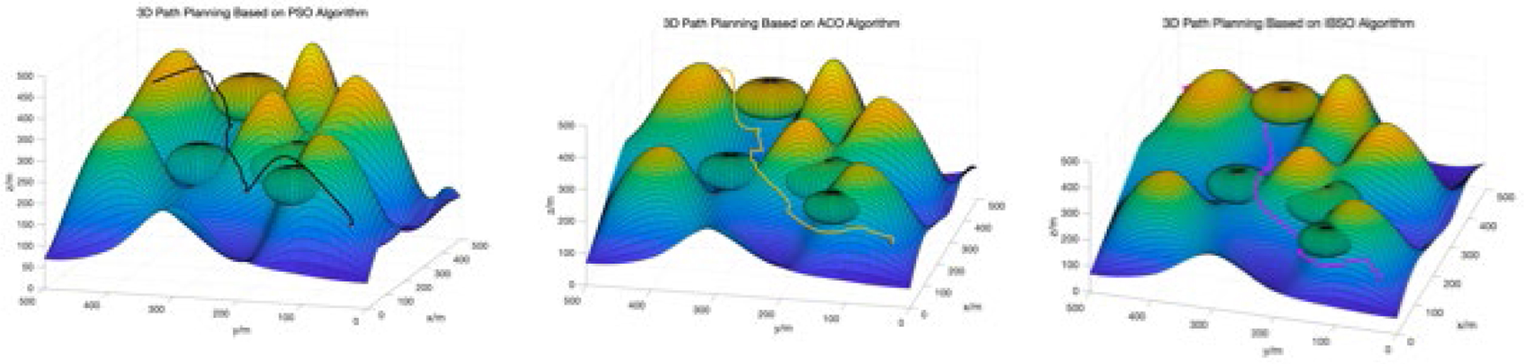
Comparison diagram of 3D path planning.

Fig. 17

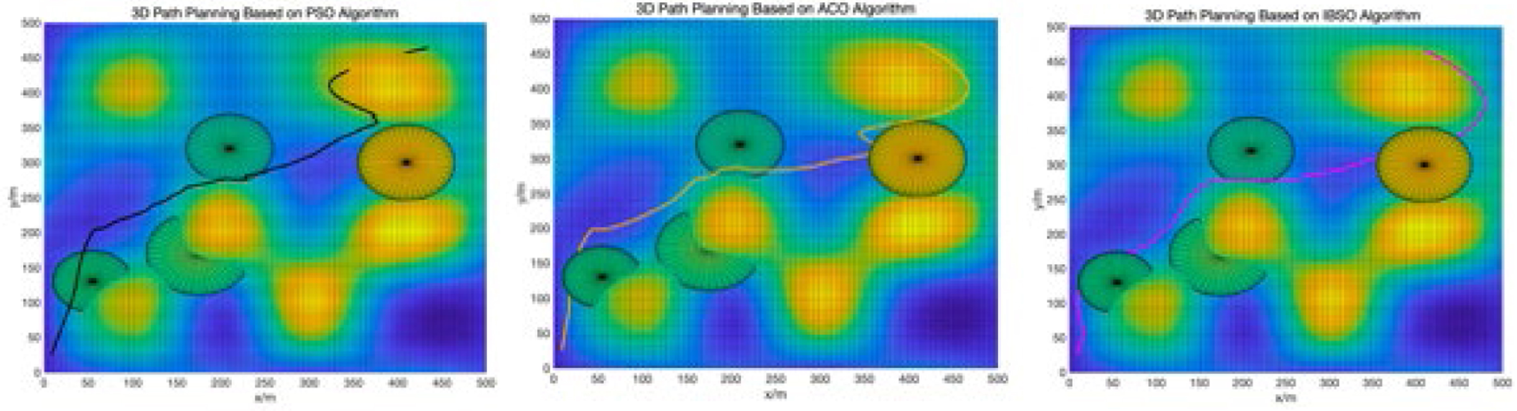
2D route diagram.

According to Fig. 16 and Fig. 17, it can be clearly seen that in the test of this case, a large number of zigzag lines appear in the trajectory of PSO algorithm in the 3D path graph. In the corresponding two-dimensional path graph, it can be found that in the later stage of operation, the trajectory of the algorithm goes into the mountains and fails to avoid obstacles. Compared with PSO algorithm, ACO algorithm does not collide with obstacles and mountains, and the route trajectory is further smoothed. IBSO algorithm has a better running effect compared with PSO and ACO. From the 3D path planning diagram and the corresponding 2D running track diagram, it can be seen that the running track is smoother with less twists and turns, and it can also successfully avoid obstacles. According to Table 15, it can be seen that the route path run by IBSO algorithm is shorter, and the simulation time is shortened to 60.3174 s, which attributes to the result of rapid optimization by the algorithm.

CASE 2: 12 peaks and 4 threats. The layout and simulation results of threat obstacles are as follows:

In order to increase the algorithm performance comparison, IBSO algorithm is used to test the three-dimensional environment of the case 2, and IBSO algorithm is tested and compared with PSO and ACO algorithm. We randomly set up 12 local highest peaks and added 4 threats to the peaks. The threats parameters and peaks parameters are shown in Tables 16 17 respectively. Path start coordinates are (15,30,210) and path end coordinates are (450,490,330).

Table 16

Threats parameters

	Obstacle center	Obstacle radius
1	(60, 200, 350)	40
2	(207, 330, 390)	40
3	(220, 180, 400)	60
4	(394, 415, 410)	50

Table 17

Peaks parameters

Parameters	h _i	x _i	y _i	x _si	y _si
1	452	358	447	8	54
2	450	250	404	12	67
3	439	146	361	9	63
4	438	350	346	9	70
5	420	244	300	14	76
6	430	450	312	13	83
7	437	150	174	8	50
8	456	283	196	10	59
9	456	400	150	11	62
10	425	100	60	16	80
11	445	200	70	10	75
12	428	310	46	9	59

The IBSO algorithm is applied to the solution of this test case, and its 3D path planning diagram and corresponding 2D path lines are shown in Figs. 18 19.

Fig. 18

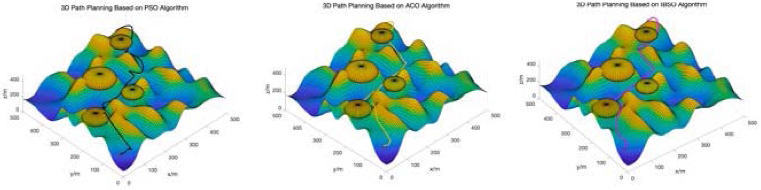
Comparison diagram of 3D path planning.

Fig. 19

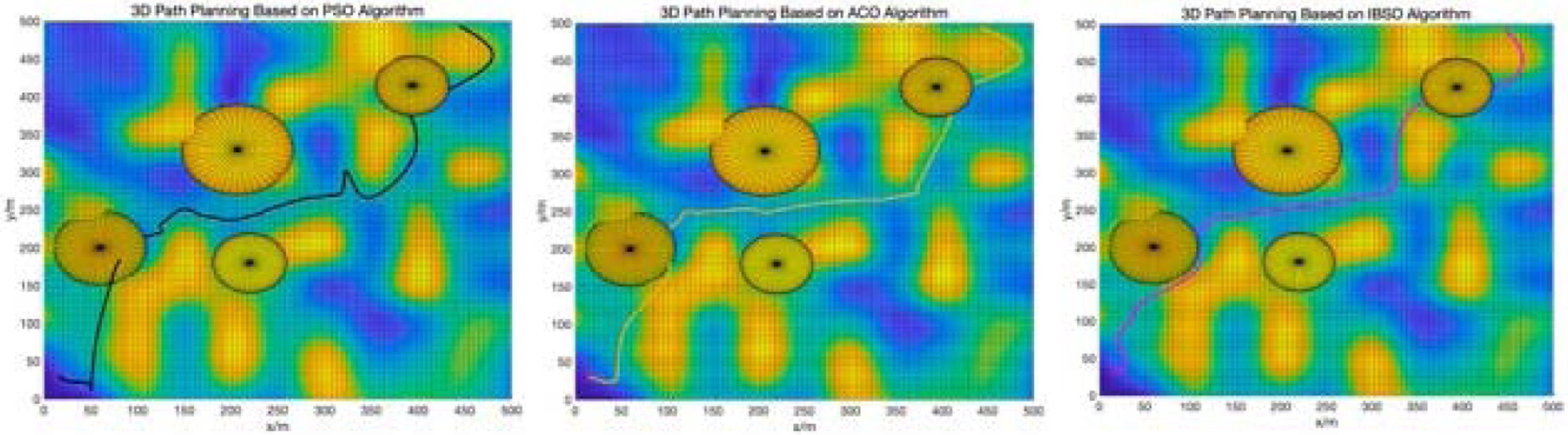
2D route diagram.

From Figs. 19 20, we can see that by solving case 2 with IBSO algorithm, we can get a smooth path that can avoid threats. At the same time, IBSO algorithm can find a path with low flight altitude. The shortest path length of the final objective function is 9.4358E+02 m. In contrast, PSO algorithm and ACO algorithm failed to avoid obstacles due to the limitation of algorithm performance when passing the first obstacle, and the path of PSO is more tortuous.

Fig. 20

Iterative diagram of path change.

For this 3D environment, each algorithm runs independently for 20 times, with 50 iterations. The average values of the detailed experimental results are shown in Table 18. The iterative comparison diagram of the three algorithms is shown in Fig. 20.

Table 18

Comparison of algorithm results

Algorithm	Path length/m	Average number of iterations to reach the optimal fitness	Simulation time/s
PSO	1008.4517	53	65.3038
ACO	964.4356	58	67.5916
IBSO	943.5891	46	59.3472

As can be seen from Table 18, the IBSO algorithm has the shortest path length, which is nearly 64 m shorter than the other two algorithms. From the perspective of test time, IBSO also has good performance, which is nearly 5s-7 s shorter than the other two algorithms. This is the embodiment of the fast iterative optimization of the BAS algorithm. The average number of iterations to reach the optimal fitness, IBSO algorithm also shows good computational performance, about 46 times can reach the optimal fitness. From the iteration comparison chart, it can be found that the final optimization result of IBSO algorithm is better than that of the other two algorithms. However, in the early iteration process, IBSO algorithm is worse than PSO algorithm and ACO algorithm, this because the random location of beetle in the initial stage of IBSO algorithm and the singularity of beetle direction will make beetle need to determine the approximate target direction in the multi-dimensional space. Once they can quickly optimize after a period of iterative optimization. Through the above experiments, we further verify the effectiveness of our IBSO algorithm in solving the obstacle avoidance problem of three-dimensional path planning.

6 Conclusion

In order to study the path planning problem, an improved beetle swarm optimization algorithm is proposed in this paper. This paper analyzes two kinds of common path planning problems: ergodic optimal path problem in discrete domain and global path planning problem in continuous domain, including traveling salesman problem, multi traveling salesman problem, path planning of two-dimensional obstacle avoidance problem and path planning of three-dimensional UAV obstacle avoidance problem. We transform the single search of traditional beetle antennae algorithm into beetle swarm search solution to enrich the global optimization. Combining with the Levy flight strategy of nonlinear sinusoidal disturbance, the single beetle is prevented from being bound by the position of local convergence, and the search space is expanded. Combined with the idea of hiring bees to search near the nectar source neighborhood in the artificial bee colony algorithm, it enriches the search ability of the beetle swarm to solve the global problem. The whole process balances the local and global search, as an improved beetle swarm optimization algorithm. We test four typical path planning problems. The experimental results show that the IBSO has better global search ability than other control algorithms, with fewer iterations, faster convergence, shorter time-consuming, and the final path is better, which provides an effective solution for the design of path planning scheme.

For IBSO algorithm we proposed, the algorithm uses random initialization during population initialization, which will cause nonuniform population distribution in the search range, and then affect the search results. In the following work, we would use Latin Hypercube Sampling (LHS), Monte Carlo method and other methods to discuss the distribution of population initialization and the solution results. Secondly, these improvements to the BAS algorithm will inevitably lead to an increase in the time complexity of the algorithm. The analysis of computational complexity also includes the spatial complexity. How the spatial complexity of IBSO algorithm changes is also the content we need to study in our future work.

In our future research, we can further optimize our algorithm from the perspective of other more complex application problems in path planning, such as the balanced traveling salesman problem and the coloring bottleneck TSP. In addition, the environment model is further improved to make it closer to the real test environment to a greater extent.

Author contributions

Conceptualization, Yucheng Lyu and Yuanbin Mo; methodology, Songqing Yue; software, Lila Hong; validation, Yuanbin Mo and Songqing Yue; writing-original draft preparation, Yucheng Lyu; writing-review and editing, Yucheng Lyu, Yuanbin Mo and Songqing Yue; supervision, Yuanbin Mo.

Informed consent statement

All authors have read and agreed to the published version of the manuscript.

Conflicts of interest

All authors disclosed no relevant relationships. All authors declare no conflict of interest.

Data availability statement

The data that support the findings of this study are available from the corresponding author upon reasonable request.

Footnotes

Acknowledgments

This work was supported in part by the National Natural Science Foundation of China under Grant 21466008; in part by the Guangxi Natural Science Foundation under Grant 2019GXNSFAA185017; in part by the Innovation Project of Guangxi Graduate Education under Grant YCSW2022255 and in part by the School Level Scientific Research Projects under Grant 2021MDKJ004.

References

Milan Erdelj

and Natalizio

, Wireless Sensor Networks and Multi-UAV systems for natural disaster management, Computer Networks 124 (2017), pp. 72–86.

Sugiyama

, Tsujioka

and Murata

, Real-time exploration of a multi-robot rescue system in disaster areas, Advanced Robotics 27(17) (2013), pp. 1313–1323.

Koparan

, Koc

A.B.

, Charies Privette

and Calvin Sawyer

, In Situ Water Quality Measurements Using an Unmanned Aerial Vehicle (UAV) System, Water 10(3), 2018.

Wang

, Wang

and Zhao

, Carrier Design and Motion Control of Marine Underwater Robot, Journal of Coastal Research 107(SI) (2020), 181–184.

Jeremy Marvel

and Norcross

, Implementing speed and separation monitoring in collaborative robot workcells, Robotics and Computer-Integdrated Manufacturing 44 (2017), pp. 144–155.

Rahmaniar

and Wicaksono

, Design and Implementation of a Mobile Robot for Carbon Monoxide Monitoring, Journal of Robotics and Control 2(1), 2021.

Kamaruddin

, Rosdi

M.N.

and Sukindar

N.A.

, Optimization of drilling path using the bees algorithm, Manufacturing Technology 21(6) (2021), pp. 788–792.

Baniasadi

, Foumani

, Smith-Miles

and Ejov

, A transformation technique for the clustered generalized traveling salesman problem with applications to logistics, European Journal of Operational Research 285(2) (2020), 444–457.

Komarudin and Chandra

, Optimization of very large scale capacitated vehicle routing problems, Proceedings of the 2019 5th International Conference on Industrial and Business Engineering Sep. 2019, Hong Kong, pp. 18–22.

10.

Geng

, Wang

and Zhang

, Motion plan of maritime autonomous surface ships by dynamic programming for collision avoidance and speed optimization, Sensors 19(2) (2019), pp. 1–20.

11.

McCammon

and Geoffrey Hollinger

, Topological hotspot identification for informative path planning with a marine robot, 2018 IEEE International Conference on Robotics and Automation (ICRA), Sep. 2018, Brisbane, QLD, Australia.

12.

Sun

and Boukerche

, Performance modeling and analysis of a UAV path planning and target detection in a UAV based wireless sensor network, Computer Networks 146 (2018), pp. 217–231.

13.

Shi

, Zhang

, Dong

and Wang

, Cruise missile path planning based on ACO algorithm and Bezier curve optimization, Journal of System Simulation 32(1) (2020), pp. 122–129.

14.

Wei

and Ren

, A method on dynamic path planning for robotic manipulator autonomous obstacle avoidance based on an improved RRT algorithm, Sensors 18(2), 2018.

15.

Chen

, Luo

, Mei

, et al., UAV path planning using artificial potential field method updated by optimal control theory, International Journal of Systems Science 47(6) (2016), pp. 1407–1420.

16.

Imad AlShawi

, Yan

, Pan

and Luo

, Lifetime Enhancement in Wireless Sensor Networks Using Fuzzy Approach and A-Star Algorithm, IEEE Sensors Journal 12(10) (2012), pp. 3010–3018.

17.

Daniel Tenezaca

, Canchignia

, Aguilar

and Mendoza

, Implementation of Dubin Curves-Based RRT* Using an Aerial Image for the Determination of Obstacles and Path Planning to Avoid Them During Displacement of the Mobile Robot, Developments and Advances in Defense and Security. Conference paper 152 (2020), pp. 205–215.

18.

Hernandez-Mejia

, Vazquez-Leal

, Sanchez-Gonzalez

and Corona-Avelizapa

, Arabian Journal for Science and Engineering 44 (2019), pp. 2321–2333.

19.

Wang

, Chu

H.E.

and Mirjalili

, Three-dimensional path planning for UCAV using an improved bat algorithm, Aerospace Science and Technology 49 (2016), pp. 231–238.

20.

Patle

B.K.

, Pandey

, Jagadeesh

and Parhi

D.R.

, Path planning in uncertain environment by using firefly algorithm, Defence Technology 14(6) (2018), pp. 691–701.

21.

Song

, Wang

and Zou

, On global smooth path planning for mobile robots using a novel multimodal delayed PSO algorithm, Cognitive Computation 9 (2017), pp. 5–17.

22.

Gemeinder

and Gerke

, GA-based path planning for mobile robot systems employing an active search algorithm, Applied Soft Computing 3(2) (2003), pp. 149–158.

23.

, Lin

, Jin

Y.Z.

, et al., A new fallback beetle antennae search algorithm for path planning of mobile robots with collision-free capability, Soft Computing 24(3) (2020), 2369–2380.

24.

and Fu

, An agglomerative greedy brain storm optimization algorithm for solving the TSP, IEEE Access 8 (2020), pp. 201606–201621.

25.

Zhong

, Wang

, Lin

and Zhang

, Discrete pigeon-inspired optimization algorithm with Metropolis acceptance criterion for large-scale traveling salesman problem, Swarm and Evolutionary Computation 48 (2019), pp. 134–144.

26.

Ebadinezhad

, DEACO: Adopting dynamic evaporation strategy to enhance ACO algorithm for the traveling salesman problem, Engineering Applications of Artificial Intelligence 92, 2020.

27.

Wang

, Zhao

, Cao

, et al., Vehicle routing optimum model of hazardous materials transportation under fuzzy environment, Journal of Intelligent & Fuzzy Systems 31(6) (2016), pp. 3067–3074.

28.

Trigui

, Koubaa

, Cheikhrouhou

, et al., A clustering market-based approach for multi-robot emergency response applications, 2016 International Conference on Autonomous Robot Systems and Competitions. Braganca, Portugal, (2016), pp. 137–143.

29.

Ann

, Kim

and Ahn

, Area allocation algorithm for multiple UAVs area coverage based on clustering and graph method, IFAC-PapersOnLine 48(9) (2015), pp. 204–209.

30.

Kiraly

, Christidou

, Chovan

, et al., Minimization of off-grade production in multi-site multi-product plants by solving multiple traveling salesman problem, Journal of Cleaner Production 111 (2016), 253–261.

31.

, Zhang

and Zhang

, A global path planning algorithm for fixed-wing UAVs, Journal of Intelligent & Robotic 91(3-4) (2018), pp. 691–707.

32.

Meng

, Liu

, Gao

, et al., A new bio-inspired algorithm: Chicken swarm optimization. Advances in Swarm Intelligence, ICSI 2014 (2014), pp. 86–94.

33.

Xiaobin

, Qing

, Pingping

, et al., An improved wolf pack algorithm, Control and Decision 32(7) (2017), 1163–1172.

34.

and Li

, BE-ABC: Hybrid artificial bee colony algorithm with balancing evolution. Strategy, 2012 Third International Conference on Intelligent Control and Information Processing. New York: IEEE, (2012), 13229324.

35.

Jiang

X.Y.

and Li

, BAS: Beetle Antennae Search Algorithm for Optimization Problems, International Journal of Robotics and Control 1(1), 2018.

36.

Jensi

and Wiselin Jiji

, An enhanced particle swarm optimization with levy flight for global optimization, Applied Soft Computing 43 (2016), 248–261.

37.

Shen

, Du

and Zhou

, Beetle swarm optimization algorithm with adaptive mutation, Journal of Computer Applications 40(S2) (2020), pp. 1–7.

38.

Karaboga

and Basturk

, On the performance of artificial bee colony (ABC) algorithm, 8(1) (2008), 687–697.

39.

Van den Bergh

and Engelbrecht

A.P.

, A Cooperative approach to particle swarm optimization, IEEE Transactions on Evolutionary Computation 8(3) (2004), 225–239.

40.

Dhiman

and Kaur

, STOA: A bio-inspired based optimization algorithm for industrial engineering problems, Engineering Applications of Artificial Intelligence 82 (2019), pp. 148–174.

41.

Mirjalili

, The ant lion optimizer, Advances in Engineering Software 83 (2015), pp. 80–98.

42.

Wang

, Zhang

and Yu

, A discrete particle swarm optimization algorithm for solving TSP under dynamic topology, 2019 IEEE International Conference on Cybernetics and Intelligent Systems (CIS) and IEEE Conference on Robotics, Automation and Mechatronics (RAM). Bangkok, Thailand, 2019.

43.

Lin

and Chen

, An improved algorithm for single-cluster TSP based on ACO, International Journal of Engineering Intelligent Systems 28(4) (2020), 197–204.

44.

Jin

, Yun

and Liang

, Improved cat swarm optimization for solving traveling salesman problem, Application Research of Computers 34(12) (2017), 3607–3610.

45.

Yang

, Zheng

and Ma

, Improved cat swarm optimization for solving traveling salesman problem, Application Research of Computers 34(12) (2017), 3607–3610.

46.

Yang

and Wang

, Multi-scale quantum free particle optimization algorithm for solving travelling salesman problem, Journal of Computer Applications 40(5) (2020), pp. 1278–1283.

47.

TSPLIB [EB/OL]. [2018-06-25]. https://comopt.ifi.uni-heidel-berg.de/software/TSPLIB95/tsp//

48.

, Ma

, Zhang

, Zhou

and Liu

, Firefly Algorithm Solving Multiple Traveling Salesman Problem, Journal of Computational and Theoretical Nanoscience 12(12) (2015), pp. 1277–1281.

49.

Zhou

, Song

and Pedrycz

, A comparative study of improved GA and PSO in solving multiple traveling salesman problem, Applied Soft Computing 64 (2018), pp. 564–580.

50.

Hengyu

, Jiqing

, Quanzhen

, et al., An improvement of fruit fly optimization algorithm for solving traveling salesman problems, International Conference on Information and Automation (ICIA) Hailar, China, July 2014, pp. 620–623.

51.

Akhand

M.A.H.

, Akter

, Sazzadur Rahman

, et al., Particle swarm optimization with partial search to solve traveling salesman problem, 2012 International Conference on Computer and Communication Engineering (ICCCE), Kuala Lumour, Malaysia. July 2012, pp. 118–121.

52.

Osaba

, Carballedo

, Diaz

, et al., On the influence of using initialization functions on genetic algorithms solving combinatorial optimization problems: a first study on the TSP. 2014 IEEE Conference on Evolving and Adaptive Intelligent Systems (EAIS), Linz, Austria. July 2014, pp. 1–6.

53.

Laha

, A quantum-inspired cuckoo search algorithm for the traveling salesman problem. 2015 International Conference on Computing, Communication and Security (ICCCS). Pointeaux Piments, Mauritius. December 2015, pp. 1–6.

54.

Pengfei

, Tao

, Guangxu

, et al., UCAV Path planning based on improved chaotic bee colony algorithm, China Sciencepaper 3(16) (2021), pp. 301–306.

55.

Wang

, Wu

, Lin

, Li

, et al., A new trajectory-planning beetle swarm optimization algorithm for trajectory planning of robot manipulators, IEEE Access 7 (2019), pp. 154331–154345.

56.

Sanchez-Lopez

J.L.

, Wang

, Miguel Olivares-Mendez

, et al., A real-time 3D path planning solution for collision-free navigation of multirotor aerial robots in dynamic environments, Journal of Intelligent & Robotic Systems 93 (2019), pp. 33–53.

57.

Kaur

and Shankar Prasad

, Path planning of multiple unmanned aerial vehicles based on RRT algorithm, Advances in Interdisciplinary Engineering (2019), pp. 725–732.

58.

, Yan

, Chu

, Cai

, et al., A new hybrid algorithm based on golden eagle optimizer and grey wolf optimizer for 3D path planning of multiple UAVs in power inspection, Neural Computing and Applications, 2022.

59.

Goel

, Varshney

, Jain

, Maheshwari

, et al., Three dimensional path planning for UAVs in dynamic environment using glow-worm swarm optimization, Procedia Computer Science 133 (2018), pp. 230–239.

60.

Elbanhawi

, Simic

and Reza Jazar

, Continuous path smoothing for car-like robots using B-Spline curves, Journal of Intelligent & Robotic Systems 80 (2015), pp. 23–56.

		Algorithm
Functions	Result	PSO	BAS	STOA	ALO	ABC	IBSO
f ₁	Best	3.441E-09	5.038E-06	1.069E-21	7.131E-15	1.377E-23	0
	Worst	1.531E-07	1.752E-05	4.253E-17	3.814E-13	4.823E-22	1.050E-159
	Mean	2.173E-08	7.177E-06	5.419E-20	5.228E-14	5.898E-23	3.776E-239
	Rank	5	6	3	4	2	1
f ₂	Best	0.0074	1.723E-06	0.0078	0.0823	0.0614	0
	Worst	0.0298	1.110E-05	0.0366	0.2904	0.1283	0
	Mean	0.0193	5.348E-06	0.0188	0.1133	0.1093	0
	Rank	4	2	5	3	6	1
f ₃	Best	1.794E-07	1.030E-07	7.956E-19	3.225E-12	1.002E-20	0
	Worst	9.552E-05	2.088E-05	1.176E-16	5.825E-10	8.127E-20	2.346E-130
	Mean	5.682E-06	1.844E-06	5.738E-18	9.322E-11	4.691E-20	1.494E-172
	Rank	6	5	3	4	2	1
f ₄	Best	1.528E-09	9.206E-07	7.632E-23	6.613E-13	1.224E-22	1.667E-304
	Worst	9.552E-07	1.845E-05	7.816E-20	1.989E-11	9.340E-22	4.171E-101
	Mean	1.563E-08	4.960E-06	1.802E-22	2.360E-12	4.461E-22	4.249E-284
	Rank	5	6	2	4	3	1
f ₅	Best	–1	–0.9323	–1	–1	–1	–1
	Worst	–0.9962	–0.5747	–0.9362	–0.9362	–1	–1
	Mean	–0.9999	–0.8247	–0.9845	–0.9845	–1	–1
	Rank	1	6	1	1	1	1
f ₆	Best	9.524E-13	5.087E-13	1.020E-23	6.963E-16	1.065E-27	1.654E-319
	Worst	1.785E-10	5.504E-12	7.573E-21	4.134E-14	1.463E-24	1.299E-151
	Mean	2.602E-11	4.462E-12	1.444E-21	8.992E-15	3.069E-25	3.039E-267
	Rank	6	5	3	4	2	1
f ₇	Best	3.145E-09	1.249E-09	0	1.359E-15	0	0
	Worst	1.379E-08	6.684E-03	0	2.196E-13	0	0
	Mean	9.342E-09	7.334E-04	0	1.596E-14	0	0
	Rank	6	5	1	4	1	1
f ₈	Best	1.367E-13	2.024E-06	5.754E-32	3.031E-12	1.748E-35	0
	Worst	6.552E-09	9.189E-05	5.102E-26	9.318E-09	1.560E-34	6.578E-150
	Mean	7.793E-10	3.576E-05	5.608E-27	2.169E-09	6.984E-35	6.696E-152
	Rank	4	6	3	5	2	1
f ₉	Best	1.893E-13	2.080E-12	9.720E-32	3.404E-15	2.346E-55	6.489E-191
	Worst	9.383E-09	2.983E-03	1.385E-27	1.968E-13	2.687E-52	7.950E-76
	Mean	1.061E-09	3.351E-04	2.824E-28	6.063E-14	4.412E-53	7.954E-77
	Rank	5	6	3	4	2	1
f ₁₀	Best	4.151E-07	0.9980	7.105E-15	1.9899	0.8427	0
	Worst	1.253E-04	7.5814	2.0829	4.9748	2.4303	0
	Mean	2.680E-05	3.8263	0.8019	3.2547	1.6271	0
	Rank	3	5	2	6	4	1