A novel fault tolerance based load balancing technique in cloud computing

Abstract

Cloud computing has emerged as one of the most promising technologies for meeting rising computing needs. However, high-performance computing systems are more likely to fail due to the proliferation of components and servers. If a sub-system fails, the entire system may not be functional. In this regard, the occurrence of faults is tolerable using an efficient fault-tolerant method. Since cloud computing involves storing data on a remote network, system failures and congestion are the most common causes of faults. The paper presents a new approach to adopting a fault-tolerant mechanism that adaptively monitors health to detect faults, handles faults using a migration technique, and avoids network congestion. With the advantage of the Ant Colony Optimization (ACO) algorithm and active clustering, the load is distributed evenly in data centers. Simulation results indicate that our algorithm outperforms previous algorithms regarding total execution time and imbalance degree up to 10% and 17%, respectively.

Keywords

Cloud computing fault tolerance load balancing energy efficiency

1 Introduction

In recent decades, Information Technology (IT) and the Internet have affected every aspect of modern society, ranging from communication to management and business to industry, specifically advances in the Internet of Things (IoT) [1], cloud computing [2], artificial intelligence [3–5], machine learning [6–9], smart grids [10], Blockchain [11], 5 G connectivity [12]. Cloud computing is one of the most significant trends in recent years. It has paved the way for distributed systems to become large-scale computing networks [13, 14]. A wide range of cloud computing services is provided to consumers worldwide by companies such as IBM, Amazon, Yahoo & Google. This paradigm enables end users to access applications on-demand rather than installing them locally on their computers [2]. Cloud computing has presented several challenges. Among the challenges, load balancing is a significant one [15]. As the name implies, it describes workload distribution between machines. It involves distributing the needed burden among multiple computer solutions and clusters, including servers, networks, disks, CPUs, etc [16]. The load balancing approach maximizes device performance, resource usage, and system output. Data or files can be easily stored and accessed by customers in an easy and scalable manner. Due to the growing demand for real-time computing, the availability and reliability of cloud computing infrastructure have become increasingly critical [16]. Cloud computing systems are more likely to fail than other computing systems. The ability to tolerate faults is one of the most important components of a high-availability and reliable cloud computing environment [13].

Fault tolerance can be implemented in two ways: reactive and proactive [17]. A proactive technique anticipates and predicts, whereas a reactive strategy reacts and responds. Using a virtual machine replacement algorithm, reactive fault tolerance techniques terminate overloaded hosts by extending the migration time in the cloud data center. As network conditions change, flexible fault tolerance switches from proactive to reactive mode. In adaptive fault tolerance, cloud resources are chosen based on cloud load [18]. Cloud infrastructure can withstand faults with adaptive fault tolerance. Data centers are made up of small units called cloudlets. It allows cloud users to access services quickly [19]. Since the load balancing issue in cloud computing has been considered an optimization NP-hard issue, it has absorbed a lot of attention. It has been solved by various heuristic and meta-heuristic algorithms. Therefore, this paper proposes a load balancing mechanism using the Ant Colony Optimization (ACO) algorithm, which increases based on dynamic and reactive characteristics and equates the tasks among involved nodes in cloud computing. Considering two types of ants and forming active clustering according to pheromones connections, the high-load or low-load nodes are quickly identified. The objectives of the paper are as follows:

Optimizing and maximizing resource utilization using the ACO algorithm

Reducing communication cost using the ACO algorithm

Minimizing the idle times for the computing nodes using active clustering

Optimizing energy consumption using ACO algorithm based on active clustering

The content of the paper is structured as below. The relevant work in the cloud computing load-balancing field is described in the next section. The load balancing strategy and the details of the suggested strategy using the developed ACO with active clustering are presented in Section 3. The analysis and simulation results are illustrated in Section 4. Section 5 concludes the paper.

2 Related works

Abdulhamid, et al. [18] propose an algorithm based on the dynamic clustering league championship algorithm (DCLCA) that increases resource efficiency and reduces untimely failures in cloud task execution. According to experimental results, the proposed technique significantly reduces the task failure rate. The proposed approach reduced the makespan by 58%, 54%, 25%, and 14% compared to MTCT, MAXMIN, ACO, and NSGA-II. Under the second scenario, the makespan was reduced by 60%, 38%, 31% and 31%. DCLCA facilitates fault-tolerant scheduling, which improves the performance of the cloud environment.

Gupta, et al. [20] suggested a technique that integrates fault tolerance with encryption algorithms. Data is encrypted before transmission using the triple-DES algorithm to improve security. Using the implemented method, encrypted data is transmitted to the node with the lowest fault tolerance. Therefore, this method uses an effective classification technique. The nodes are classified based on their similar content and features using a support vector machine classifier (ISVM). In conjunction with the ISVM, it is possible to predict the faults early on, before they occur. The proposed system takes into account three parameters, availability, reliability, and accuracy. Fault tolerance accuracy is improved by 79% over the existing system.

Hasan and Goraya [21] propose an adaptive fault-tolerant model for cloud computing. The system enables users to classify tasks as economy, standard, or premium in order to apply fault tolerance at the appropriate level. The fault tolerance level is implemented by executing user tasks on a cooperative resource group in the cloud. Keeping the deadline guarantee ratio and average task delay for a variety of task categories demonstrates the flexibility of the proposed framework. A comprehensive set of simulation experiments is conducted on artificial and real workloads to analyze and compare the performance of the framework regarding fault tolerance capability, resource consumption, and utilization.

The proactive fault tolerance system proposed by Ray, et al. [17] preempts faults within a federation based on CPU temperature. Within the federation, fault tolerance is modeled as an optimization problem problem to maximize profit and minimize migration costs by redistributing resources from faulty providers to non-faulty providers. As a solution to this issue, Preference-Based Fault Management (PBFM) is developed to manage faults within the federation. This mechanism is evaluated and compared with other mechanisms in extensive experiments. The proposed mechanism is shown to yield an optimal solution in the presence of faulty cloud service providers for the general trade-off problem of profit and migration costs.

Attallah, et al. [15] propose a mechanism that tolerates virtual machine CPU faults in order to maximize the availability and reliability of cloud computing infrastructure. It tracks CPU utilization changes and decides when a high CPU utilization value is detected. A virtual machine can be migrated from one destination host to another, or the loads can be managed on the destination host so they can be migrated. Whenever the destination host becomes overloaded, the load balancing subroutine is launched; otherwise, the load is calculated.

Rezaeipanah, et al. [22] developed a fuzzy-based approach for error tolerance based on an analysis of the nature and detection of errors. Error tolerance and load balancing are improved by re-executing tasks and moving through checkpoints in the event of an error. Due to the time-consuming nature of migration techniques, the use of checkpoints can help avoid tasks from having to be re-executed. Experiments show that the proposed method outperforms the ABFT algorithm by 6.49% and the FFD algorithm by 2.27% for the accuracy criterion.

3 The load balancing strategy

Load balancing architecture and its basic properties are described in this section.

3.1 Proposed dynamic and elasticity load balancing architecture

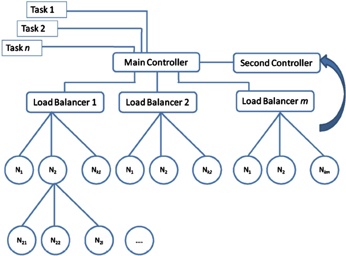
A useful load-balancing policy should be performed and optimized to the nearest data center and the vast requests. As shown in Fig. 1, the load-balancing architecture consists of three main layers. The first layer contains the primary and secondary controls. The primary control is the first element to receive the task of users based on precedence, area, and technical features, and then these tasks will be sent to the balance zone. Moreover, the central controller is orderly associated with the second controller, so the information is provided to update the system status. The secondary controller must communicate quickly with the load balancing area to update the system status information. The secondary balance updates the various nodes through various factors according to the load level. Therefore, the central controller will be in the state of correction and declare the frequency of different levels of the load node. This configuration is designed to decrease the load on the controller. The second layer is the load balancing layer. The components perform different tasks sent by the control manager and adjust the received messages through different cloud nodes, adopting the ant colony optimization algorithm. Two levels of nodes form the third layer, the first of which catches the tasks submitted by local load balancing. The tasks are then performed to reduce the size of user requests based on the main tasks. The findings of Taguchi have shown that “factor size” has a remarkable effect on response time.

Fig. 1

The dynamic and elasticity load balance proposed.

According to the proposed cloud computing platform and architecture, the ACO algorithm, like cloud nodes, has several features in common with data repositories for nests and load allocation for food activities.

3.2 Forward and backward ants

The preceding ant begins to discover the nominated nodes to balance the load on the cloud computing platform and look for its activity from the production node. The candidate nodes include 1 – max-min load nodes and sub-nodes. Backward ants update their pheromone information according to their orientation [23]. These ants are produced continuously by forward ants and recognize a nominated node. As defined in [24], the forward ant in each neighbor computes the possibility of a move and then selects the largest one for its next goal. In order to speed up the convergence, a particular strategy is added to the model once backward and forward ants are placed in the same node. The mentioned strategy performs by calculating the pheromone info and the pheromone node about the backward ants [25]. A timer is used to record the post-production cycles of ants to simulate the accumulation. Each node has some storage units to save pheromone info by ants at the rear sight with one unit for an ankle. Two ant sorts only meet once in a moment. The ant is assumed to be in a node before the ants are behind the node. When the timer reaches zero, the pheromone data given by the ant will be cleared. If each node includes more than one ant, all their effects must be calculated, while the possibility of continuing that node is measured.

3.3 Maximum – minimum rules

This part defines two separate rules called max – min order for ant production.

First rule: Maximum startup rule (trigger, relay circuit):

If this node exceeds the threshold once, a forward ant from the sub-node will be produced. To optimize resource utilization, the node must be distributed among empty nodes as it approaches its maximum load.

Second rule: Startup rule (minimum value):

If a node in this node is less than one threshold, a sub-node will be generated. This process allows the node to handle numerous novel tasks for sharing resources with excessive nodes under a light load. According to the mentioned tactics, the load balancing main stages are as below:

Calculate the possibility of a move for all neighbors and choose the largest one as the next goal.

Moving to a novel node to determine if the node is nominated or not. If yes, a reverse ant will be created. Step 1 applies to a forward ant.

Ants going backward start at the same place as forwarding ants going forwards: updating the pheromone information of ants bypassing and removing the ants as they reach the beginning position.

Demand time can be balanced by calculating the total resources available at the candidate node and stopping if sufficient resources are available.

The load is balanced.

These steps are equivalent to the maximum rules except for the method of calculating the probability of movement in section 4.

3.4 Modeling of dynamic and elasticity load balancing with ant colony system optimization

Following the strategy outlined above, this section provides more information about the probability of moving with ant colony optimization. Two significant problems should be solved to evaluate network efficiency: First, the prioritization of pheromones in cloud computing must be logical to comply with the desired quality of service. Second, the pheromone should be updated with the dynamic demand for diversity and the goal of accelerating convergence.

3.4.1 Initial start of pheromones

The resources assigned to virtual nodes in cloud computing are not similar and often change dynamically. As explained above, physical machines are used to measure the resources’ initial nodes [16, 26, 27]. CPU, I/O interface and bandwidth, internal storage, and external storage are five physical sources involved in the primary pheromone. Equation 1 is used to calculate the CPU capability. $p_{CPU} = n \times p$ (1)

A limitation should be set for each parameter to simplify the calculation. When the parameter has a high value, a limited amount is opted for instead of the real value. The constraints are shown in the equation (2).

$\begin{matrix} p_{CPU} < p_{\max}, m_{i} ⩽ m_{imax}, m_{e} ⩽ m_{emax}, \\ p_{i / o} ⩽ p_{i / omax}, p_{b ⩽} p_{bmax} \end{matrix}$ (2)

The following equations are the definition of the physical resources of virtual machines.

CPU: $τ_{CPU} (0) = \frac{p_{CPU}}{p_{\max}} \times 100 %$ (3)

Internal storage: $τ_{mi} (0) = \frac{m_{i}}{m_{imax}} \times 100 %$ (4)

External storage: $τ_{me} (0) = \frac{m_{e}}{m_{emax}} \times 100 %$ (5)

I/O interface: $τ_{i / o} (0) = \frac{p_{i / o}}{p_{i / omax}} \times 100 %$ (6)

Bandwidth: $τ_{b} (0) = \frac{p_{b}}{p_{bmax}} \times 100 %$ (7)

Therefore, the first value of pheromone to a sub-node is defined as below: $\begin{matrix} τ_{i} = Ψ_{1} τ_{CPU} (0) + Ψ_{2} τ_{mi} (0) + \\ Ψ_{3} τ_{me} (0) + Ψ_{4} τ_{i / o} (0) + Ψ_{5} τ_{b} (0) \\ \sum_{n = 1}^{5} Ψ_{n} = 1 \end{matrix}$ (8)

In equation (8), ΨN is the weighting coefficient for regulating the effects of physical resources in cloud calculations.

3.4.2 Updating pheromones

In fact, the goal of updating pheromones is to collect the values of pheromones for nodes that are taken in a good situation and reduced in adverse circumstances. The evaporation of pheromones, updating work, and motivation for performing prosperous tasks effectively update pheromones.

3.4.3 Evaporation of pheromones

Due to the pheromone reduction by evaporation in the node over time, a local update strategy is used. The subgroups are used to change the pheromones when their rate is not zero. The following definition is for updating the pheromones by evaporation: $τ_{i} (t + 1) = (1 - ρ) \times τ_{i} (t), 0 < ρ < 1$ (9)

Here, τ_i (t) is pheromone at node T, and P is a coefficient for vaporization.

3.4.4 Evaporate pheromone

Once the function of a sub-node is altered, a novel task will be assigned to this node. Once new tasks are received due to resource consumption, the ability of this sub-node is reduced. Here, the pheromone is updated by: $τ_{i} (t + 1) = (1 - μ) \times τ_{i} (t), 0 < μ < 1$ (10)

Here, μ refers to the determinant of the resources consumption. The functionality of the sub-node changes over time as new tasks is performed. By disseminating resources, this node enhances its capacity. Under these circumstances, the following equation calculates the amount of pheromone. $τ_{i} (t + 1) = (1 + v) \times τ_{i} (t), 0 < v < 1$ (11)

Here, v is the agent for fast control of the resources.

3.4.5 The evaporation of pheromone for the rear ant

As noted in the previous sections, the rear pheromones are controlled under the nodes stored by the timer. Over time, the pheromones are evaporated like the natural pheromones of nodes. Updating the pheromones with the utilization of evaporation for the rear ants is calculated as: $τ_{i} (t + 1) = (1 + π) \times τ_{i} (t), 0 < π < 1$ (12)

Here, π indicates the rear ant’s coefficient of evaporation.

3.4.6 Motivational and punitive laws

Two motivational rules and a punishment law are defined for performing a slave job. If the tasks for success increase, the pheromones in this node will also increase. If the task fails, the pheromone in this node will decrease. Updating the pheromones is calculated by this rule: $\begin{matrix} τ_{i} (t + 1) = (1 + θ) \times τ_{i} (t) \\ if (success) 0 < θ < 1 \\ else - 1 < θ < 0 \end{matrix}$ (13)

Here, θ is the agent for regulating the amount of motivation and the punishment for the taken nodes.

3.4.7 The task of forecasting implementation

In fact, the performance prediction is used to assess the speed of running a sub-node and the efficiency of virtual resources in cloud computation. The total cloud platform yield improves with better performance of assigning tasks to sub-nodes. In this paper, the prediction model is designed to speed up node execution and frame evaluation by gathering the prior records. With the contemporary workload at the last time, the speed of a sub-node can be calculated for the next time, when frame using the following formula:

$\begin{matrix} {EV}_{i}^{a_{k + 1}} (k + 1) = \\ \frac{a_{k + 1}}{a_{k}} ((1 - ω) {EV}_{i}^{a_{k}} (k) + ω {RV}_{i}^{a_{k}} (k)) \end{matrix}$ (14)

Here, with regard to ${EV}_{i}^{a_{k}} (k),$ the KTH speed is predicted to run the work on the node i and the AK workload KTH in this node. ${RV}_{i}^{a_{k}} (k)$ refers to the real speed of KTH. Ω is a customizable parameter for weight control used for real implementation and prediction. Over time, the contemporary tasks decrease while the prediction of work speeds up; therefore, the prediction speed of the work must be raised during the tasks performed at regular intervals as follows: ${EV}_{i}^{a_{k + 1}} (t + 1) = (1 + σ) {EV}_{i}^{a_{k + 1}} (t)$ (15)

Here, σ is the parameter related to the gain control degree in the direction predictable by the work.

3.4.8 The rules for moving of forwarding ant

In this way, there are two situations where the forward ants calculate the possibility of moving to the next destination. One of the situations is that there are no ants in the neighboring nodes, and the fact is that one or more ants appear in the neighboring nodes. In this section, these two items are evaluated.

3.4.9 Without an appearing of ant in the adjacent nodes

As explained in the previous part, in different conditions, the ants are used to search for unnecessary nodes. Therefore, two aspects of ants are discussed in the neighboring nodes.

(1) The forward ant is inserted too much by the nodes: In this condition, it is possible to move the forward ant using: $p_{ij} = {\begin{matrix} \frac{{[τ_{ij} (t)]}^{a} {[{EV}_{ij}^{a_{k + 1}} (t)]}^{β} {[η_{ij} (t)]}^{γ} {[D_{ij} (t)]}^{κ}}{\sum_{j ɛ N_{n}} {{[τ_{ij} (t)]}^{a} {[{EV}_{ij}^{a_{k + 1}} (t)]}^{β} {[η_{ij} (t)]}^{γ} {[D_{ij} (t)]}^{κ}} \\ ifj ɛ N_{n} \\ 0 \end{matrix}$ (16)

Here, p_ij indicates the likelihood of the ant moving across nodes i to j. N_n is a collection of neighboring nodes, τ_ij (t) is the j pheromone, ${EV}_{ij}^{a_{k + 1}} (t)$ is the prediction speed of running the work in the j node, and η_ij (t) refers to the cost of moving from node i to node j, i.e., the degree of node j divided by the sum of its neighbors: $D_{ij} = \frac{d_{j}}{\sum_{k ɛ {NB}_{i}} d_{k}}$ (17)

Here, NB_i is the neighboring node of node i, which is more likely to be selected by a node with a maximum degree in the next destination.

(2) The forward ant is reduced by the following node: By calculating the possibility of moving forward in this situation, a decision can be made: $p_{ij} = {\begin{matrix} \frac{{[η_{ij} (t)]}^{γ} {[D_{ij} (t)]}^{κ}}{\sum_{j ɛ N_{n}} {[η_{ij} (t)]}^{γ} {[D_{ij} (t)]}^{κ}} \\ if j õ N_{n} \\ 0 \end{matrix}$ (18)

Here, the equivalent parameters of equation (16) have the same similarities except for the deletion of TIJ (T) and ${EV}_{ij}^{a_{k + 1}} (t)$ .

3.4.10 Rear assembly ant neighboring node

Upon placing the forward ant at the original node, the pheromone transferred by the backward ant must be taken into account. In a node with multiple ants, the entire pheromone left behind by each ant must be included in the pheromone. This case requires consideration of two conditions in turn.

(1) The probability of movement by extra nodes is as follows: $p_{ij} = {\begin{matrix} \frac{{[τ_{ij} (t) + \sum τ_{b} (t)]}^{a} {[{EV}_{ij}^{a_{k + 1}} (t)]}^{β} {[η_{ij} (t)]}^{γ} {[D_{ij} (t)]}^{κ}}{\sum_{j ɛ N_{n}} {[τ_{ij} (t) + \sum τ_{b} (t)]}^{a} {[{EV}_{ij}^{a_{k + 1}} (t)]}^{β} {[η_{ij} (t)]}^{γ} {[D_{ij} (t)]}^{κ}} \\ ifj ɛ N_{n} \\ 0 \end{matrix}$ (19)

Here, ∑τ_b (t) refers to the total amount of pheromones released by the backward ant. The values of other parameters are also similar to those in equation (16).

(2) The forward ant is reduced by the following node:

As mentioned previously, the probability of motion is calculated using equation (18).

3.5 Optimization formulation

Then, the issue of optimizing the virtual machine placement is formulated. Suppose that n virtual machine (applications) i ∈ I must be placed on the m server j ∈ J. For clarity, it is imagined that no virtual machine needs more resources than the resources provided by a server. Suppose that R_{p
_i} requires the CPU of each virtual machine, T_{p
_j} is the threshold for using CPU about each server, R_{m
_i} is the memory demand of virtual machines, and T_{m
_j} is the threshold for using the memory of servers. Two dual variables, x_ij and y_j are used. The x_ij bin variable shows if the virtual machine i is specified to the j server and the dual variable or not. The y_j variable indicates whether the j server is used or not. Reducing the consumed time and eliminating the resources simultaneously are the main goals. Therefore, the placement problem can be as follows: $\begin{matrix} Minimize \sum_{j = 1}^{m} P_{j} = \sum_{j = 1}^{m} y_{j} \\ \times ((P_{j}^{busy} - P_{j}^{idle}) \times \sum_{j = 1}^{m} (x_{ij} . R_{p_{i}}) + P_{j}^{idle}) \\ Minimize \sum_{j = 1}^{m} W_{j} = \sum_{j = 1}^{m} \\ [y_{j} \times \frac{| (T_{P_{j}} - \sum_{i = 1}^{n} (x_{ij} . R_{p_{i}})) - (T_{m_{j}} - \sum_{i = 1}^{n} (x_{ij} . R_{m_{i}})) |}{\sum_{i = 1}^{n} (x_{ij} . R_{p_{i}}) + \sum_{i = 1}^{n} (x_{ij} . R_{m_{i}})}] \end{matrix}$

With the goal of $\sum_{j = 1}^{m} x_{ij} = 1 \forall i \in I$ (20) $\sum_{i = 1}^{n} R_{p_{i}} . x_{ij} ⩽ T_{p_{j}} . y_{j} \forall j \in J$ (21) $\sum_{i = 1}^{n} R_{m_{i}} . x_{ij} ⩽ T_{m_{j}} . y_{j} \forall j \in J$ (22)

In Equation (20), we defined the specificity of a server for a virtual machine within a range. Any virtual machine can be applied to one server and does not serve multiple servers. Equation (21) and (22) show limitations for server capacity. It means that the server exchanges information with the virtual machine. In other words, the dedicated capacity between the server and the virtual machine has limitations. The variable problems that may happen in the cloud environment are considered constraints. Continuous disconnection and connection conditions, manipulation conditions for a specified period, etc., that may occur are considered. There are possible solutions for MN to proceed with a virtual machine for a collection of M physical machines and N virtual machines. In this way, it is generally impossible to have a full census of total feasible remedies to detect the best remedies. Subsequently, there is an illustration of how a colonial ant system is used to find the appropriate solutions for large solution spaces.

3.6 Explanation of the suggested ant colony optimization algorithm

The suggested algorithm for solving the issues described in the preceding sections stands on the ant colony system. A complete solution to the problem of a multivariate virtual machine is considered a virtual machine allocation permutation. The terms “host” and “server” in this article will be utilized interchangeably. Assigning a virtual machine to the host is called a move and is shown by a virtual machine host.

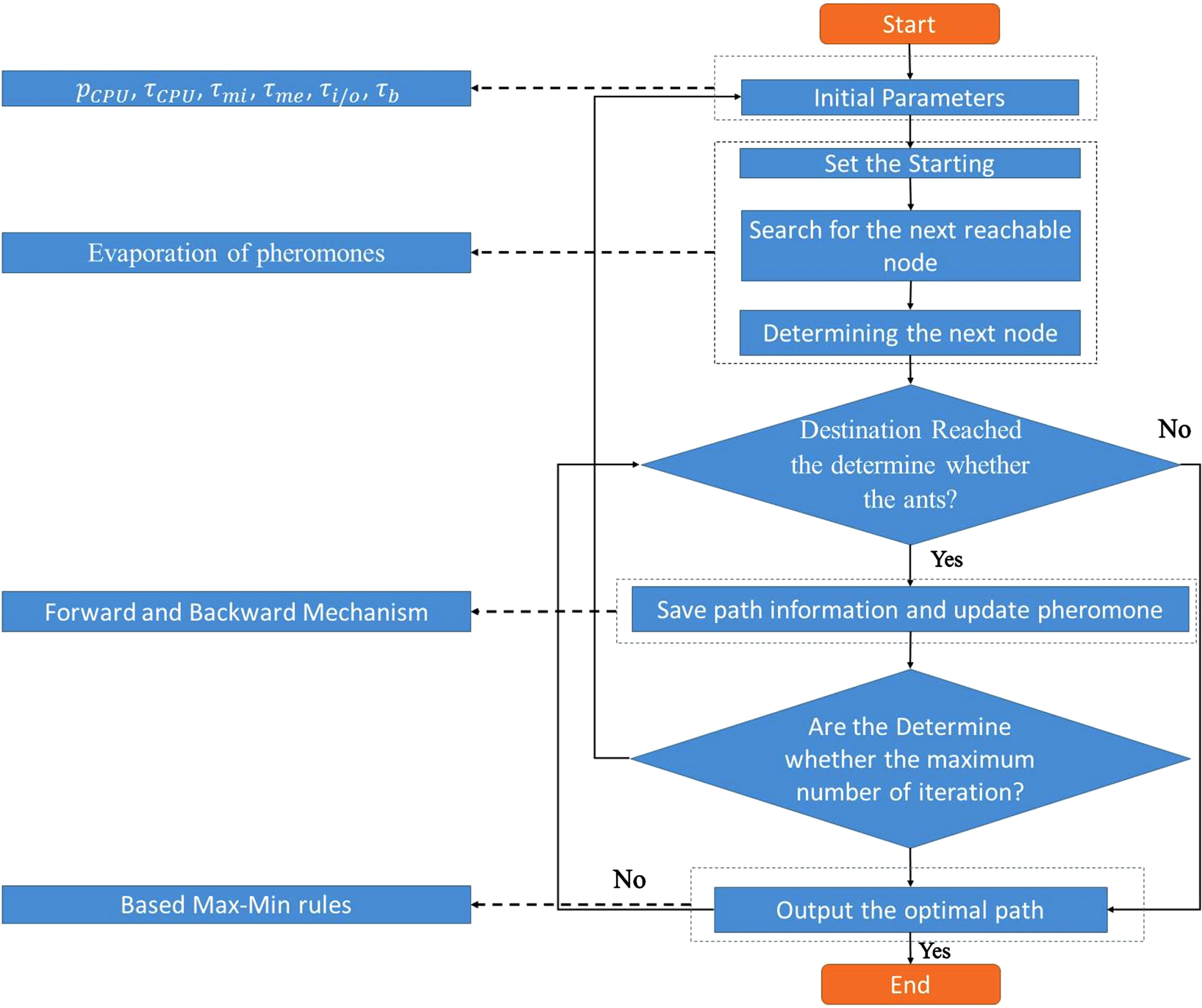
Figure 2 illustrates the proposed ant colony algorithm. At the initial step of the algorithm, the parameters and total pheromone paths are set to “T0”. Each ant gets all virtual machine demands in the iteration section, presents a physical server, and starts allocating the virtual machine to the host. This procedure is accomplished by utilizing a pseudo-random-proportional rule that explains the utility of an ant for selecting a particular virtual machine as the next virtual machine to accommodate its contemporary host. This law is about the pheromone focus in motion and a heuristic that directs the ants to the most hopeful virtual machines. An update to local pheromones is conducted when an artificial ant performs a move. The ants have formed their remedies, and the universal updates are done with each solution from the contemporary beam set.

Fig. 2

The closed ant process flowchart.

3.6.1 Description of pheromone sequence and exploratory data

With the general implementation of ant colony algorithms, the virtual machine of the ant colony system begins with the pheromone path matrix and exploratory matrix. The quality of the ant colony system performance mostly depends on the explanation of the pheromone sequence meaning [28]. It is essential to select an explanation that meets the specification of the topic. Two different pheromone forms should be considered: one that links a pheromone sequence with each virtual machine-host motion or the other that connects the pheromone sequences to each pair of virtual machines. In this article, the first step is to plot the pheromone paths; for example, the pheromone sequence TI. j defines the tool for adapting the virtual machine i to host j. In the first stage, the pheromone surface is calculated by τ₀ = 1/[n · (P′ (S₀) + W (S₀))], in which n is the virtual machine number, S₀ is the remedy produced by the exploratory FFD, and W (S₀) is the loss of S₀ solution resources. The P′ (S₀) consumption of normalized time is the S₀ solution, and its rate can be calculated based on the following equation (23): $P^{'} (S_{0}) = \sum_{j = 1}^{m} (P_{j} / P_{j}^{Max})$ (23)

The $P_{j}^{Max}$ is the peak in consuming j server time.

3.6.2 Making a solution

In the allocation process, the K-ant, according to the pseudo-accidental rule, selects a virtual machine i as the next destination to suit its contemporary host. $i = {\begin{matrix} \underset{u \subset Ω_{k (j)} {α \times τ_{u, j} + (1 - α) \times η_{u, j}}, q ⩽ q_{0}}{argmax} \\ s . otherwise \end{matrix}$ (24)

Where A is known as a parameter that enables the applier to control the pheromone sequence significance. Here q₀ is an accidental number, which is distributed equally in [0, 1]. If q is larger than q₀. This procedure is known as exploration, unlike exploitation. q₀ is a constant parameter 0 ⩽ q₀ ⩽ 1 that determines the importance associated with the accumulated knowledge exploitation of the subject compared to identifying new movements shown in equation (24).

3.6.3 Updating the pheromone sequence

Another vital component of an ant colony system is updating pheromone routes. The pheromone sequence value may be increased due to the ant pheromone or reduced by the evaporation of the pheromone. The situation that the pheromone sequence must illustrate the data gathered in some suitable solutions is that the placement of the new pheromone is in a standing position, and this solution, as a profit one by other ants, estimates the next solution. However, the vaporization of pheromones provides a useful form of oblivion. In the suggested algorithm, the pheromone updates the process consisting of two levels: updating the local pheromone and updating the global pheromone. In accordance (25) equation, when constructing a virtual machine assignment to host j, the ants minimize the level of pheromone sequence between the host j and virtual machine i using local update law. $τ_{i, j} (t) = (1 - ρ_{l}) τ_{i, j} (t - 1) ρ_{l} . τ_{0}$ (25)

3.7 Dynamic scheduling strategy

Scheduling refers to assigning tasks among available computational resources, considering particular objectives. Since cloud environments are rapidly evolving, dynamic scheduling methods have been developed to generate a group of independent tasks in a computationally sized set or task segments/clusters using task properties that focus on a priority or a partition. These methods schedule cluster tasks across finite resources in heterogeneous clouds. An innovative algorithm with knowledge of the restricted resources available in the cloud environment is used to classify task clusters. To improve resource accessibility computation, task clustering and mapping are combined into a shared resource allocation method. This method does not prioritize dynamic scheduling to achieve fault tolerance and load balancing. Consequently, due to the heterogeneous and dynamic nature of cloud resources, the need for an active clustering scheduling method to reflect these changes becomes a challenging problem.

3.7.1 Cloud system

Cloud systems are generally composed of heterogeneous distributed sources. Utilizing virtualization technology, physical machines (PMs) can typically hold multiple virtual machines (VMs). VMs are the key processing unit in cloud systems. To fulfill the different needs of the user, cloud services offer different types of VMs at different prices.

3.7.2 Governing strategy at scheduling methods in cloud environment

Task scheduling methods based on intelligent fault-tolerant algorithms play a central role in cloud environments in avoiding task errors due to cloud resources’ heterogeneity and dynamic nature. The current method has been evaluated using four different real-world scientific workflow scenarios to show the power of this method. This method consists of a static scheduler that uses workloads inputs to be executed on the task graph before implementation and an unrealistic dynamic scheduler that transfers processes during execution if redundancies are unnecessary. Simulation outcomes show that compared to task replication methods or current VM, the proposed method can reduce the overall error rate of programs by more than 50% and the total energy overhead by about 76%. Nevertheless, this method uses a duplication approach that could impact system performance and dynamic scheduling policies. In order to avoid errors due to overload or VM failure, it is necessary to use current cloud resources at any point in the schedule. Existing dynamic scheduling methods either do not take into account fault tolerance and load balance parameters or are applied in part at different scheduling levels.

3.7.3 Fitting function in the proposed algorithms

Cloud providers strive to decrease completion time, whereas customers aim to reduce cloud resource access costs. Therefore, the fitness value can be calculated using equation (26). $f (C) = \max {\cup_{i = 1}^{m} C_{i}}$ (26)

Where $C_{i}^{'}$ denotes the completion of task i. The shorter completion times result in better algorithm performance, i.e., less time is spent running the algorithm. According to Equation (27), Expected Completion Time (ETC) is the amount of time it takes to perform a task on a given virtual machine. The value of the multiplication tasks in the value of the resources determines matrix dimensions, and their elements are shown as ETC (Ti, Vk). ETC matrix related to this problem with n task T = {T1, T2, …, Tn} and m the virtual machine that displayed as V = {V1, V2, …, Vm} source. $ETC = T \cdot V = [\begin{matrix} T_{1} V_{1} & T_{1} V_{2} & \cdot & \cdot & \cdot & T_{1} V_{m} \\ T_{2} V_{1} & \cdot & \cdot & \cdot & \cdot & \cdot \\ \cdot & \cdot & \cdot & \cdot & \cdot & \cdot \\ \cdot & \cdot & \cdot & \cdot & \cdot & \cdot \\ \cdot & \cdot & \cdot & \cdot & \cdot & \cdot \\ T_{n} V_{1} & \cdot & \cdot & \cdot & \cdot & T_{n} V_{m} \end{matrix}]$ (27)

An error rate is equal to Pf (ji, rk) when security Demand (SD) and Trust Level (TL) are taken into consideration. SD refers to the security demand for tasks sent by applications. The application is more secure when SD is higher. TL, or trust model, evaluates VM site reliability. Differences between machine security and task demand define a task error model. Equation (28) expresses the probability of an error related to the scheduling of a task T with a specific SDj value, in VMi with a TLi trust value. TL represents the security of VM resources. The higher the TL value, the greater the VM reliability. In Equation 28, α is the error coefficient which is a fractional number. 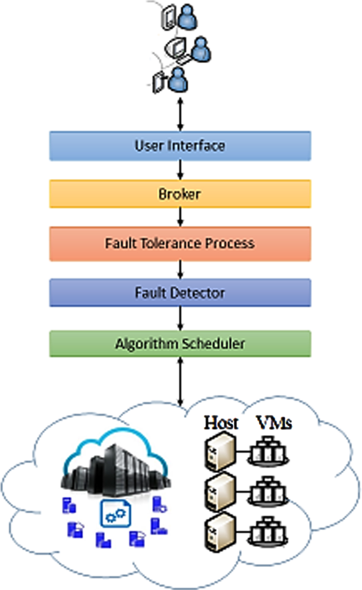$P_{f} (T_{i}, V_{k}) = {\begin{matrix} 0, {ifSD}_{i} ⩽ {TL}_{k} \\ 1 - e^{- \propto ({SD}_{i} - {TL}_{k})}, \\ if {SD}_{i} ⩽ {TL}_{k} \end{matrix}$ (28)

3.8 Components of fault tolerance scheduling method and load balancing

Figure 3 illustrates the scheduling component for fault tolerance awareness and load balancing. Each component is explained in detail in this section, along with its simultaneous operation.

Fig. 3

Fault tolerance scheduling components.

3.8.1 Fault detector and recognizer

Fault tolerance and load balancing mechanisms require error detectors as a fundamental requirement. Many error detection algorithms emphasize certain metrics such as performance, coverage, and error complexity. Existing error detection methods, classified by system-level hierarchy, use the proposed fault-tolerance algorithm scheduling method to detect errors at the operating system, application, and virtual machine levels. Execution of tasks on virtual machines can be observed remotely, and task faults can be identified through abnormal internal implementation details. Virtual machine detection can be accomplished by installing a detection component in virtual machine managers (VMMs) that alternately identifies VM errors. One of the error detection tasks we present here is to track the VM or the error task. It then schedules the repair sub-module in sequence with an ACO repair or recovery scheduling algorithm. A repairing module directs the resulting repair modules to correct faults based on their severity and classification. The errors are repaired one by one until the task is completely recovered.

3.8.2 Task immigration

A task migration happens when defective resource queues are reassigned to unused resource queues. It also solves the problem of fragmentation of tasks. The migration algorithm reschedules erroneous or aborted tasks (T_n) on a VM_j virtual machine that is available or has a low load and is known as its backup base. Suspended or aborted tasks (T_n) can be immediately transferred to another VM_j for execution if some tasks have not been executed on a particular VM for some reason (such as workload or VMi error). Labor migration increases resource productivity and also offers alternative resources in the event of a VM or overhead error, as shown in Fig. 4.

Fig. 4

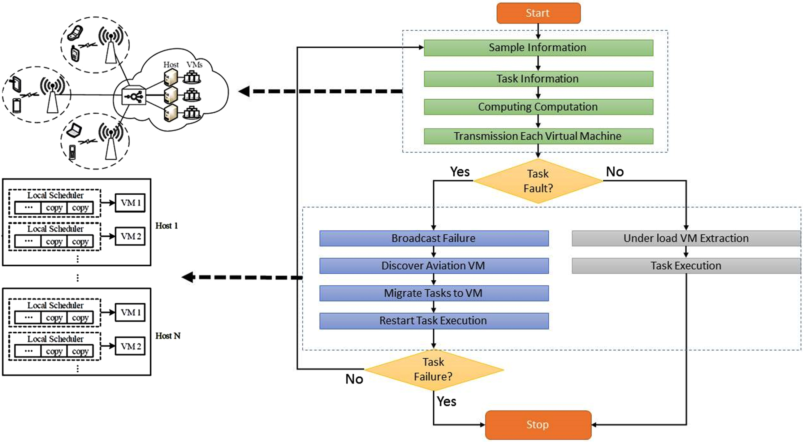
Task migration flowchart.

3.9 Clustering process in cloud environment

The active clustering task scheduling method is based on a proposed algorithm inspired by nature. As specified in Fig. 5, the Active Clustering method is used to update and reflect the current state of cloud VM resources.

Fig. 5

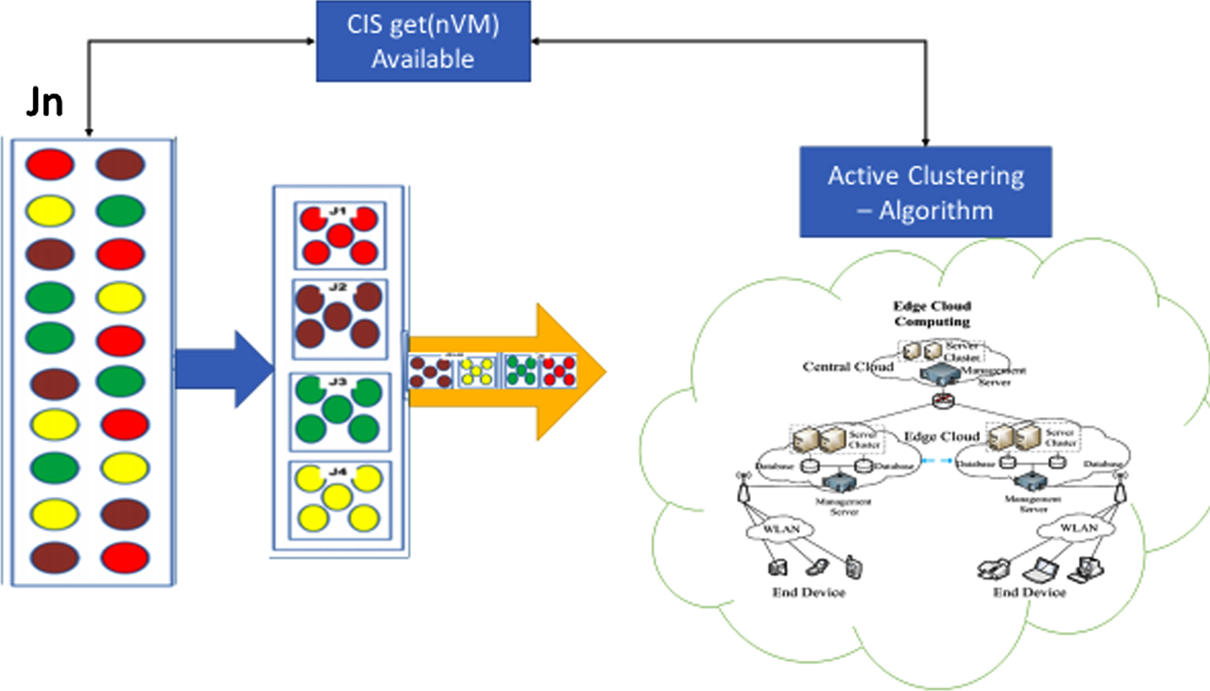
Active clustering of tasks.

3.9.1 Task clustering

A primary goal of task clustering is to distribute tasks dynamically across available virtual machines. Consider a subset of the functions j_n ∈ J where pn, P_n ={j₁, j₂, j₃ … , jn} represent a part of J in n clusters. $j_{i} \neq Ø i = 1, 2, 3, \dots, n$ $j_{i} \cap j_{j} = Ø i, j = 1, 2, 3, \dots ni \neq j$ $\cap_{i = 1}^{n} j_{i} = J$

This clustering step aims to identify the best task cluster for VM mapping using the Cloud Information System (CIS), which provides dynamic access to the number of VMs available, the anticipated implementation time, and the VM capacity. Conversely, as a result of task and resource dynamics features, cluster volume is uncertain for richer use. At each stage in the schedule, the available CIS information is utilized to identify the number of available VMs to dynamically separate tasks according to the number of available resources.

3.9.2 Active clustering mechanism

Dynamic clustering models using activated and parallel processes have been introduced to overcome the limitations of existing distributed and parallel approaches. The active clustering (AC) model combines the features of hierarchical clustering and partitioning techniques. It does not have the problem of the number of partitions being predetermined nor the problem of stopping hierarchical clustering conditions (Partitioning-based clustering). Clusters are dynamically calculated and hierarchically generated. These features seem very promising, and this method has been evaluated on a very small scale. This paper focuses on large-scale AC implementation based on the ant colony pattern. The main purpose is to prove that the AC method can benefit from a flexible, distributed, and parallel environment. For example, an ant colony runs in a cloud environment. Implementing AC using the ant colony pattern leads to examining its behavior and capabilities in a large data set without compromising results. The rest of this section describes the method and its implementation using the ant colony programming model.

The dynamic, active clustering method includes two main stages (1) the local model, in which a local clustering is created, and (2) the global model, in which interfering local clusters are combined to produce global clusters. However, exchanging the local clusters with the network nodes creates substantial overhead, which makes the process much slower. Most distributed clustering methods suffer from this problem. Therefore, exchanging the minimum number of points between nodes is recommended. Accordingly, their index points are exchanged instead of sending all the data points of the clusters, which contain 1% to 2% of the total data set size. The density and shape of a spatial cluster are the best way to illustrate it. As shown in Fig. 6, the cluster’s shape is specified by its boundary points (known as contour). The algorithm of α for creating cluster boundaries is based on triangulation. This is an effective algorithm to create non-convex boundaries, which can detect a wide range of densities and distribute different points with reasonable complexity O (n log n).

Fig. 6

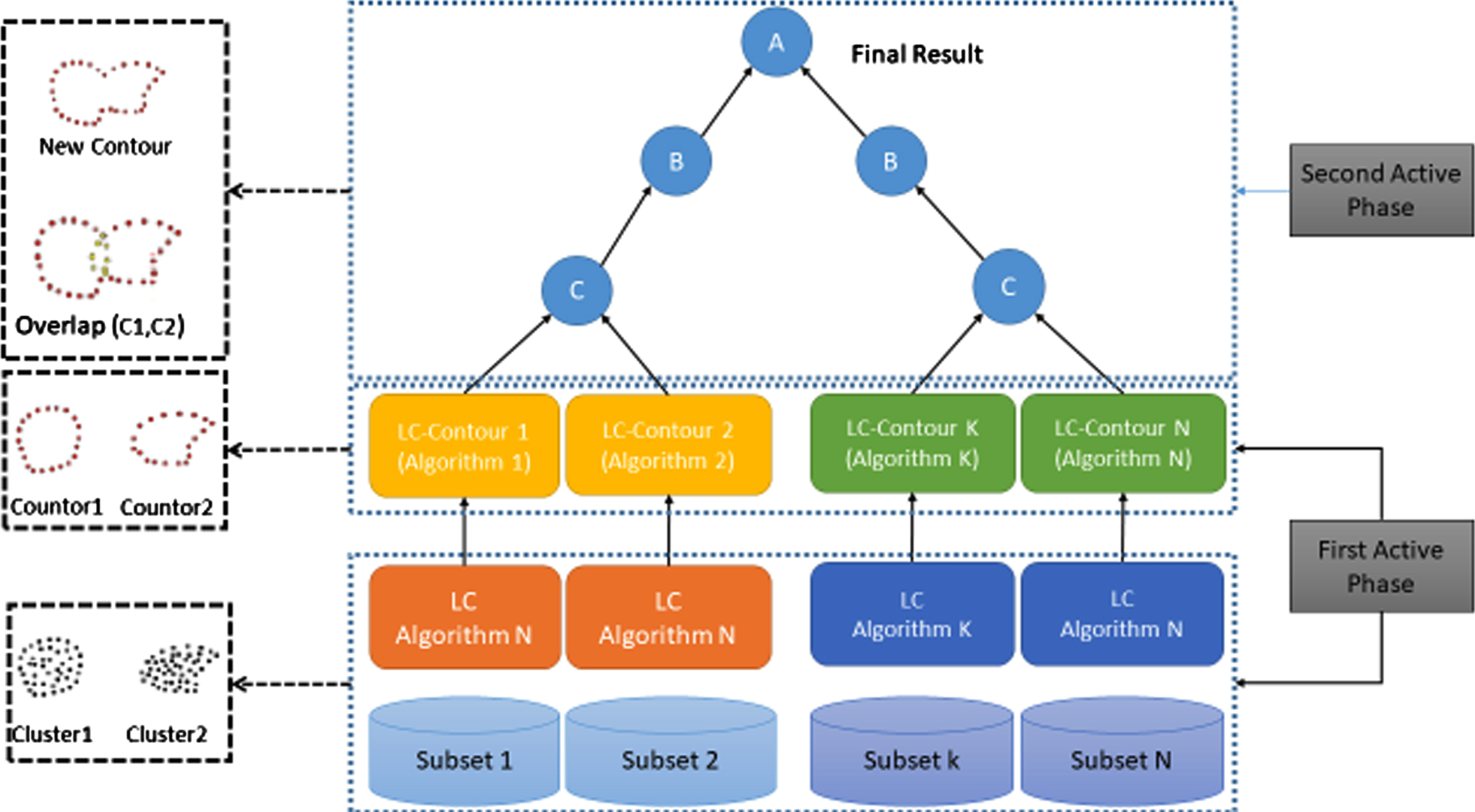
Flowchart active clustering mechanism.

Using an ant colony, the AC method has two stages, including mapping and decline. Clustering algorithms are run by mappers, and contour algorithms are then used to extract index points from local clusters. In the second stage, the contours created by the different processing nodes will be integrated among the local interfering clusters. The mapping and decline stages are conducted simultaneously. Nodes are clustered locally, and contours are calculated in parallel without any relation between them. Reducers integrate contours hierarchically. Hierarchical levels proceed in parallel. Each level of the hierarchy ends with the involved processing nodes exchanging their cluster contours. The size of the exchanged data is very small, leading to an efficient connection.

The AC model processes data in parallel in a distributed way, which minimizes the connection among nodes. According to the current implementation, HDFS distributes data randomly among different nodes. Hadoop manages the distributed and parallel specifications of the algorithm. The mappers operate independently and implement diverse clustering algorithms to explore their local data sets. The decline stage starts as soon as the contours are received. The repetition of sensory data is very important to build a reliable cloud-IoT infrastructure. In the event of server failure, sensory data assure feedback to stimuli. The backup system can handle any failure of the backup system. The Availability Zone (AZ) is a backup in case of server failure. The edge computing technique enables IoT applications to run locally rather than in the cloud. Therefore, mist and fog-level servers must have sibling backup servers to keep the program running in the event of any server edge failure. Multilevel architecture is a reliable proposition. In other words, there is a guarantee of repetition at a higher level if there are no replacement servers at one level with sensory data repetition. The amount of data for the same application may be different at the cloud, fog, and mist levels.

4 Simulation analysis, results, and comparison

A cloud simulator (CloudSim 3.0.3 on the Eclipse IDE Luna 4.4.0) was used to implement and evaluate the task scheduling of the proposed ACACO fault tolerance and load balancing method. Two different scenarios were considered to simulate the proposed algorithm. In the first scenario, task tracking is generated from the parallel workload archive, which contains 85,786 tasks. This workload archive, as a standard workload format recognized by CloudSim, is made available by the San Diego Supercomputer Center (SDSC). However, task tracking in the second scenario is generated from the CloudSim PlanetLab workload. ACACO parameters are set as ψ₂ = 0.7 =ψ₁, and pc = 0.02; the selection of these values is based on.

In order to compare the effectiveness and performance of the proposed algorithm with previous works, four different scheduling algorithms are taken into account. The methods are RA and BLSV, ACO, and NSGA-II. The number of ants per colony is n = 10, the vapor agent P = 0.4, the pheromone updates constant Q = 100, exploratory information weight β= 1, and the pheromone tracking weight α= 0.3. NSGA-II parameters are set based on; Population size = 2000, maximum repetition = 2000, mutation rate = 0.2, and intersection rate = 0.6. The trials were repeated ten times for each method, and the average termination time, fault rate, fault decline, and performance improvement rate (in percent) were observed. Two scenarios of trials with the same parameter values are repeated for all selected scheduling methods.

4.1 Performance criteria

Some of the performance parameters, such as fault rate, fault decline, and performance improvement rate, are considered to assess and compare the performance of the proposed fault-tolerant task scheduling approaches. A brief description of these parameters is provided in the following.

4.1.1 Termination time

Termination time refers to the maximum completion time or the completion of the last task. Therefore, if C_ij defines the time that V_i resource requires to complete the T_j task. Therefore, ΣCi is the total time that the V_i resource completes all the tasks sent to it. Equation 1 mathematically defines the termination time in cloud environments.

4.1.2 Fault rate

The fault rate (FR) is the ratio of the sum of failed tasks in the suggested method to the sum of failed tasks in the other scheduling method. The ACO method will be improved if the FR value is less than one that d is calculated using Equation (29). $FR = \frac{\sum_{0}^{n} no . of failures (DCLCA)}{\sum_{0}^{n} no . of failures (other scheme)}$ (29)

4.1.3 Fault decline

Fault decline (FD) refers to the ratio of time lag or interruption as a result of a faulty task to fault-free implementation time divided by the average of the sum of other tasks. FD of the proposed approach should be smaller than other methods, which have been used for comparison and are calculated using Equation (30). $FD = \frac{Time delay by failure to failure free task execution time}{Average total number of tasks}$ (30)

4.1.4 Performance improvement rate

The performance improvement rate (PIR) is defined as the percentage of performance improvement (or decline in the termination time) for the proposed ACACO method and is calculated using Equation (31). $\begin{matrix} PIR (%) = (makespan (other scheme) \\ - makespan (Algorithm)) \\ \times \frac{100}{makespan (Algorithm)} \end{matrix}$ (31)

Five cloud users are generated in the first station, with two data centers and five servers. The first data center consists of three hosts, while the second consists of two hosts. Ten VMs are also generated using the time-sharing policy, in which each is BM 512 with an image size as much as BM10000, whose CPU is managed by Xen, the virtual machine manager (VMM) in the Linux operating system. The host memory is 2048 MB, with a storage capacity of 1,000,000 and a bandwidth of 10,000. Moreover, the number of tasks (small clouds) is between 10 and 100, whose length and file are 800,000 and 600, respectively. Figures 7, 8, and 9 and Table 1 indicate the results of this section.

Fig. 7

Termination time of the first scenario.

Fig. 8

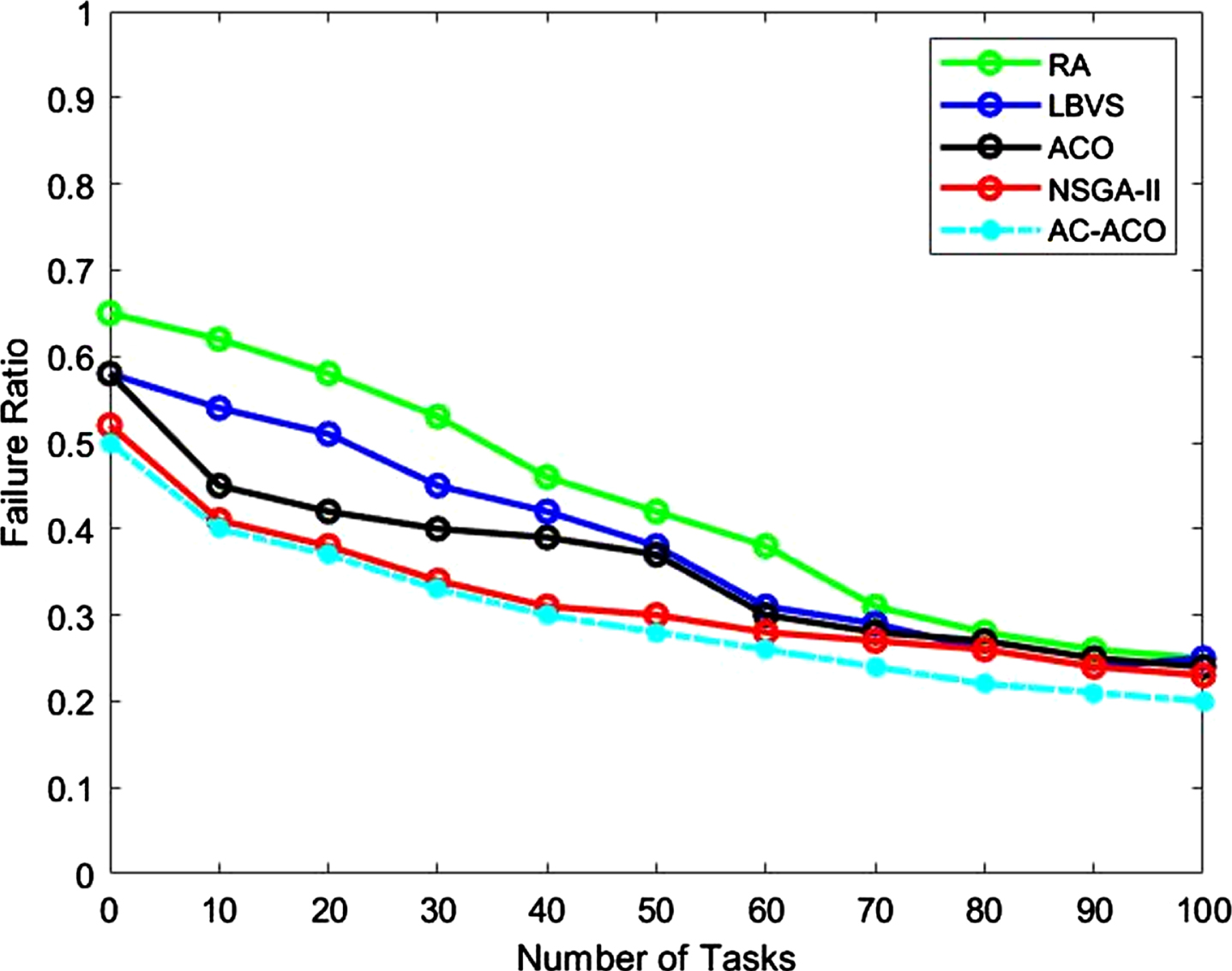
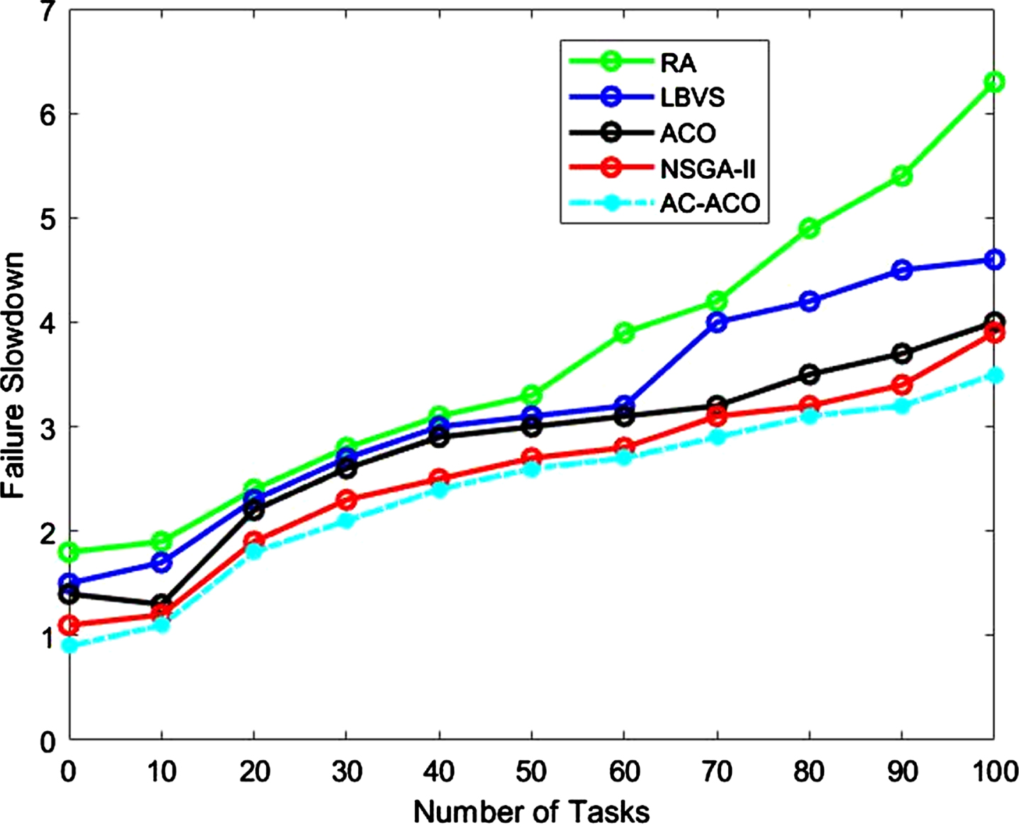
Fault rate of the first scenario.

Fig. 9

Fault decline of the first scenario.

Table 1

Performance improvement rate (%) based on the termination time

	RA	BLSVE	ACO	NSG-II	AC-ACO
Total makespan	15,063	14,285	12,085	11,856	8520.6
PIR % over RA		3.2	28.0	39.0	58.2
PIR % over BLSV			25.7	36.5	54.7
PIR % over ACO				9.7	24.6
PIR % over NSG-II					14.8

According to Fig. 7, since the number of small clouds increased in all six intended methods, the termination time (the completion time of the last task that should be performed) also increased. When a small number of tasks are sent to be implemented, all approaches have relatively the same termination time, and ACACO shows slight improvements. The termination time of the algorithms increases, and ACACO returns less time by increasing the number of tasks from 10 to 100. In other words, ACACO consumes less time to implement cloud tasks compared to the residual examining algorithms. Table 2 shows that ACACO provides PIR 59.2%, 55.7%, 26.8%, and 15.2% for RA, BLSV, ACO, and NSGA-II, respectively.

Table 2

Number of repetitions and time of convergence with different parameters

NO	μ	ν	θ	ω	Σ	α	β	γ	κ	Num	CT
1	0.2	0.2	±0.2	0.4	0.2	1	1	1	1	351	16.842
2	0.2	0.2	±0.2	0.4	0.2	1	1	2	2	324	17.308
3	0.2	0.2	±0.2	0.4	0.2	2	2	1	1	410	21.935
4	0.2	0.2	±0.2	0.4	0.2	2	2	2	2	425	22.234
5	0.3	0.3	±0.3	0.5	0.3	1	1	1	1	310	16.325
6	0.3	0.3	±0.3	0.5	0.3	1	1	2	2	298	13.586
7	0.3	0.3	±0.3	0.5	0.3	2	2	1	1	389	17.246
8	0.3	0.3	±0.3	0.5	0.3	2	2	2	2	405	18.698
9	0.4	0.4	±0.4	0.3	0.4	1	1	1	1	340	15.825
10	0.4	0.4	±0.4	0.3	0.4	1	1	2	2	315	14.324
11	0.4	0.4	±0.4	0.3	0.4	2	2	1	1	415	17.256
12	0.4	0.4	±0.4	0.3	0.4	2	2	2	2	432	22.927

Figures 8 and 9 specify the fault rate and fault decline. Moreover, the performance improvement rate is shown in Table 2. The fault rate declined with the nearest compared intelligent algorithms, while the number of tasks for all methods was increased. If the fault rate is lower, the success rate of the task will be better. Furthermore, ACACO improves the fault rate because it shows a lower ratio with increasing tasks compared to other methods. The results represent that the fault decline of the proposed ACACO method is less than the previous algorithms. The results also show that the PIR% of the suggested method is faster and better than other algorithms regarding reliability and minimum termination time. In other words, the proposed method has a higher fault tolerance, load balancing, and reliability level than the other examined algorithms. The reason may be the dynamic nature of this method, which immediately reflects the current state of available resources in a heterogeneous environment that can be resulted from its effective performance in global and local search in comparison to other meta-heuristic algorithms.

The second part of all, various tests of parameters should be performed for finding the optimal settings of the parameters. In general, the processor is most important in hardware resources [29–31], so Ψ₁, Ψ₂, Ψ₃, Ψ₄, Ψ₅ = 12 : 7 : 7 :7 : 7aredetermined. According to [32], the evaporation ratio for the sub-node is ρ= 0.5, while the ratio of evaporation for the rear ant is 0.5 = π. There are 10,000 sub-nodes on the platform cloud, and all the nodes are configured randomly with various acting potencies. The initial amount of pheromone in a node is calculated after the random assignment of the sub-nodes. Each repetition is considered as a single time in the proposed trial. At a single time, a new task with 10,000 tasks is randomly distributed to 10,000 sub-nodes. All the tasks are completed in [1, 3] units. All ants can convey an edge from one sub-node to another and update the pheromone once per unit.

During the procedure, 50 sub-nodes with a workload greater than 9 are chosen as over-loaded nodes, and 50 sub-nodes with less than two works are randomly selected as under-loaded nodes. If there are not adequate sub-nodes to respond to such situations, the real number of nodes will be over-loaded or under-loaded nodes. The forward ants are produced from over-loaded nodes and under-loaded nodes to speed up the search process. Load moderation happens when it reaches the highest search level. The highest search level is for the longest distance that ant may reach during one unit of time. After adjusting the load operation, the cloud platform reaches the unit of subsequent time, and a new task comes with 10,000 tasks.

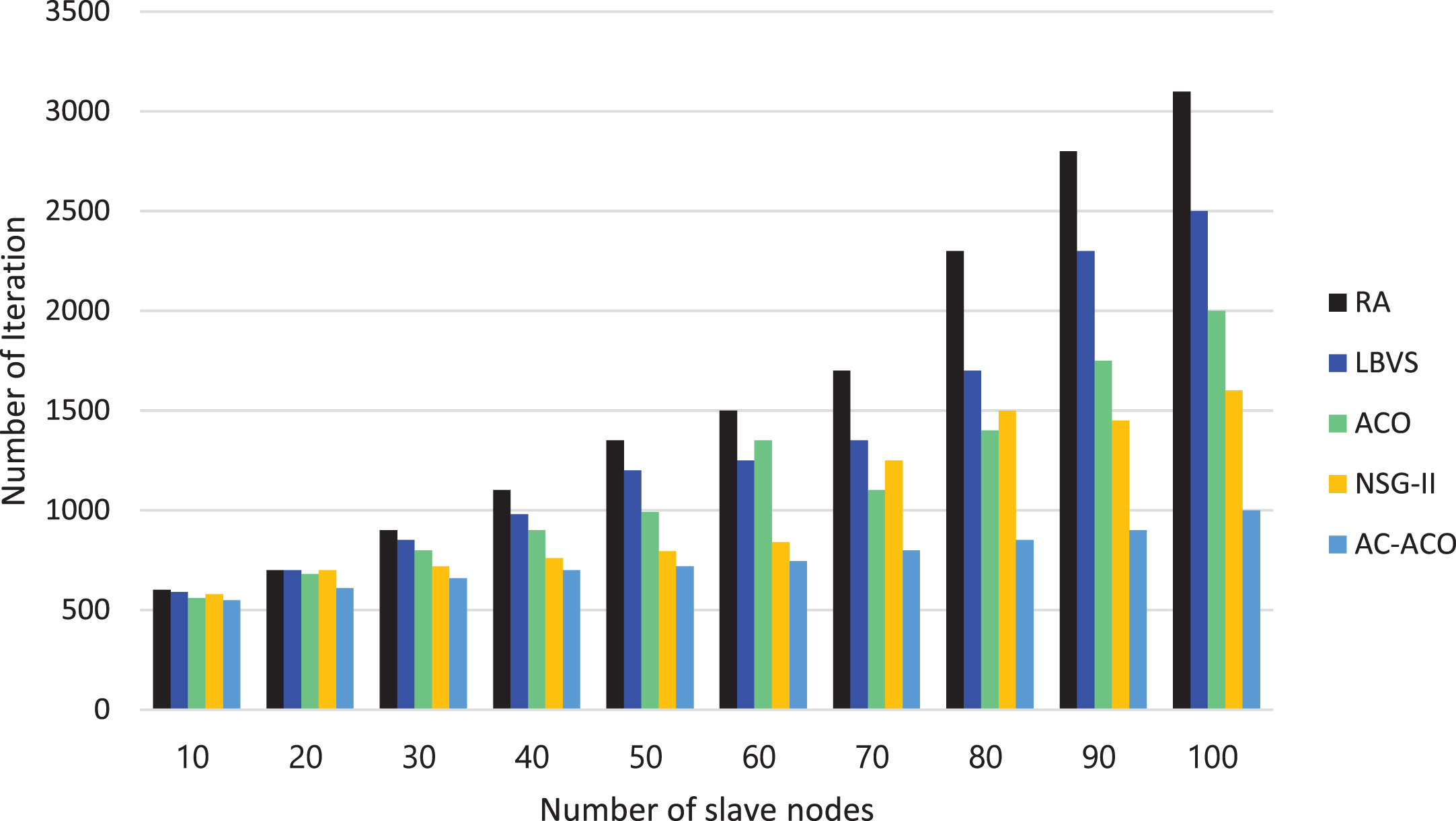
Table 2 shows the practical consequences for the repetition number (Num) and the time of convergence (CT) with different parameters when it reaches the load range. The simulation is performed 20 times for each parameter group, and CT and Num outcomes are mean amounts. Table 2 illustrates the consequences in row 6, including the lowest number of repetitions and the convergence time for achieving load modification, which means that the offered procedure can be optimized by adjusting this parameter. Therefore, this kind of settings for parameters is utilized for the following simulations.

As the number of ants affects the results, the research is performed with 100 (100-ant), 200 (300-ant), and 300 (300-ant). The maximum search level for ants is set to 10. The load balancing is used to reflect the rate of virtual machine balance on the platform of the cloud. The load adjustment degree is described as: $LB = \sqrt{\frac{1}{n} \sum_{i = 1}^{n} {({Load}_{i} - {Load}_{avg})}^{2}}$ (32)

Where Load_i is the load of the virtual machine that is the load of the sub-node and Load_avg represents the mean load of total VMs. The number of repetitions should be limited to less than 600. The simulation results of the runtime and load adjustment time with the number of ants are shown in Figs. 10 and 11.

Fig. 10

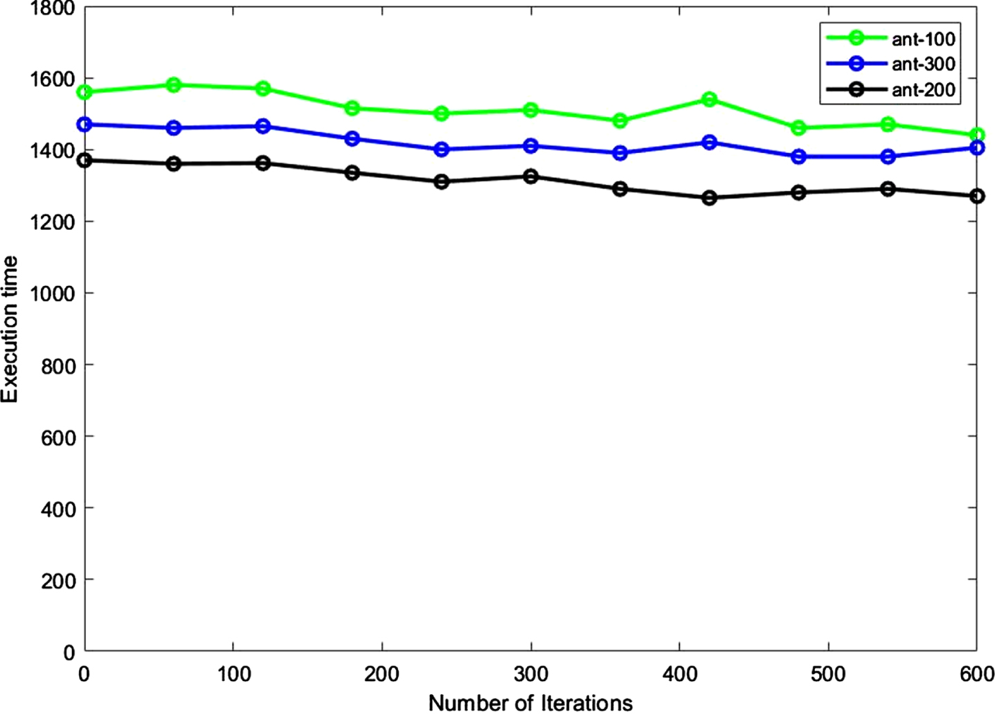
Runtime by the number of ants.

Fig. 11

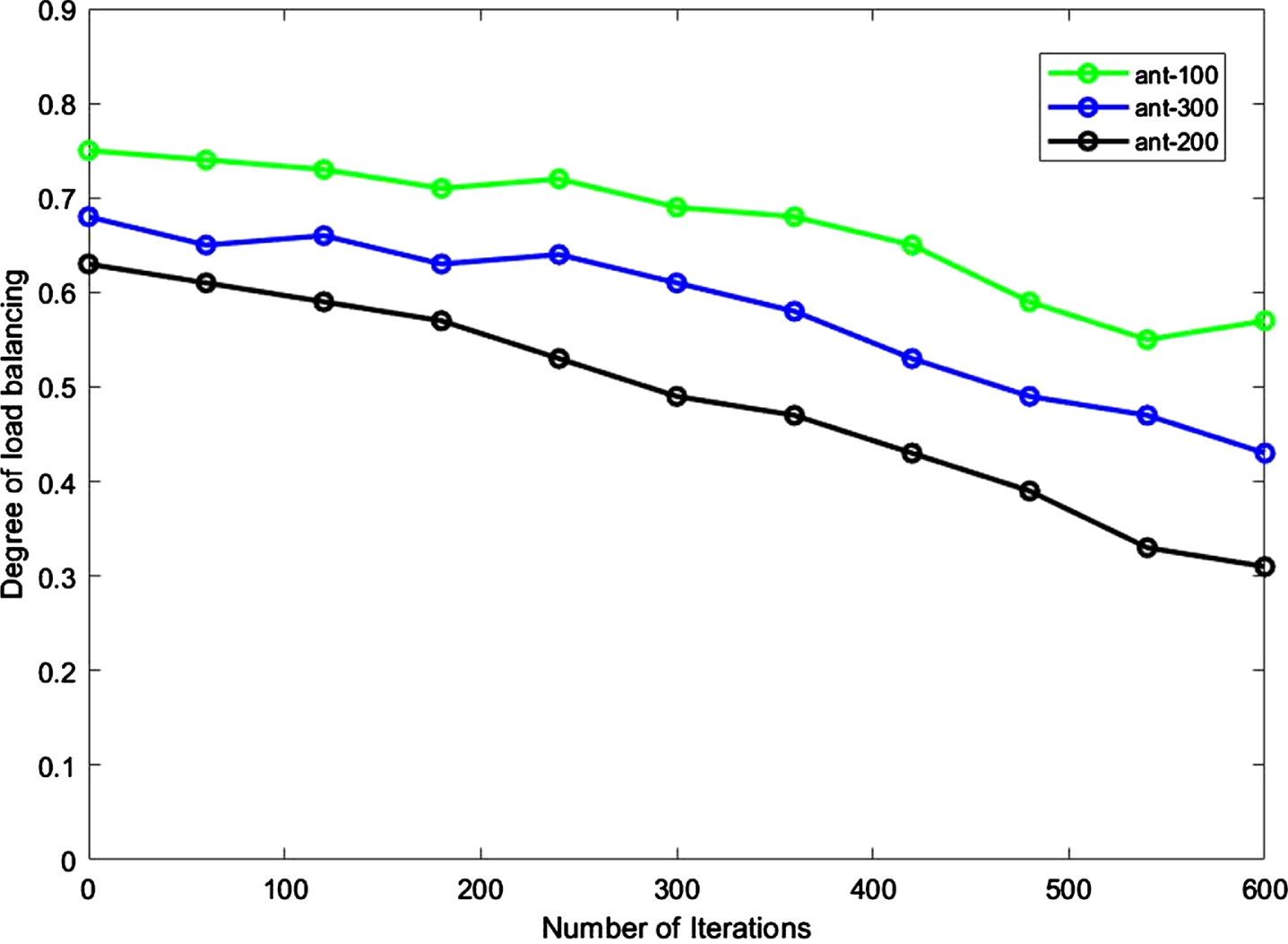
The load adjustment degree with the number of ants.

It is possible to obtain the results of minimum values for the rate of repetitions and the amount of load regulation when the ant number is set to 100. Without considering the number of ants, the highest search level for each ant affects the consequences. Therefore, various experiments with a maximum step of searching for 10 (step 10), 20 (step 20), and 30 (step 30) are performed. Figures 12 and 13 show the results of the runtime and degree of load adjustment with the maximum level of the search.

Fig. 12

The load adjustment degree with the number of ants.

Fig. 13

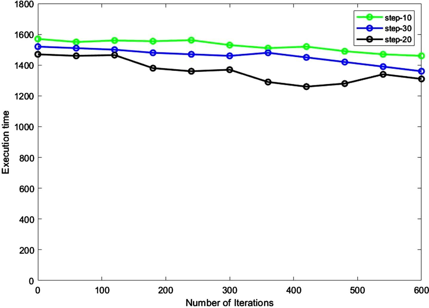
Runtime with the maximum number of different steps.

According to the results, the least search time is received when the highest search level is set to 10. Since the ants have to move forward in step 20 compared to the ants in step 10, more time is needed for ants to move forward in step 20. There is a weak act to reach the last of five steps since most ants need help finding the right sub-nodes in five steps. The experimental methods with NSG-II are used instead of the NSG-II algorithm to achieve better performance in experiments. The 100 ants are randomly distributed for random algorithms in 100 sub-nodes. At a single time, the ants record the highest and lowest sub-nodes in the search procedures and load them before the subsequent unit time. The replay number is also restricted to 600. The outcomes are demonstrated in the load adjustment degree with different algorithms in Fig. 14 and the runtime with various algorithms in Fig. 15.

Fig. 14

Load adjustment degree with a different maximum step.

Fig. 15

Runtime with various algorithms.

Fig. 16

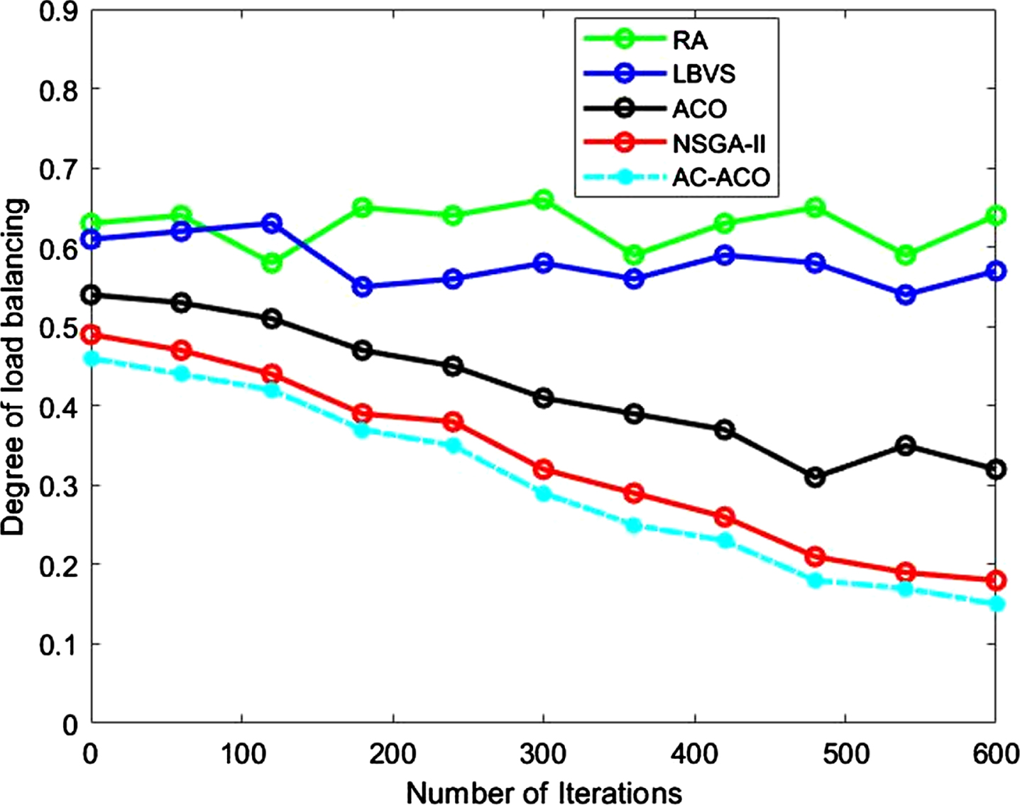
Load adjustment degree with different algorithms.

Due to the results, the convergence rate of the suggested method is better than the others, and this method can be applied to cloud computing involving many sub-nodes. Our proposed method reaches its global minima in the 200th iteration, and the makespan remains the same. Comparative algorithms, however, find global minima after 300 iterations. This indicates that our algorithm converges quickly and is stable, meaning that it can find the global minima within a relatively small number of iterations and maintain that minimum even with further iterations. Therefore, our proposed load balancing method is more efficient from the computational complexity perspective. The random process is an unpredictable algorithm due to its high instability and runtime. Although the LBVS has a volatile random algorithm, it is better than an accidental algorithm. Therefore, the suggested approach is proper for load regulation in cloud computing that can handle assigning dynamic tasks on the cloud system. The suggested procedure has better action and less time than a random method and the LBVS algorithm. It can increase the cloud platform and the speed of convergence over time.

5 Conclusion and future work

Cloud Computing is an emerging technology for the provision of services such as, facilitating the easy access to data, programs, and files via the Internet (cloud), and providing scalable storage online rather than on users’ computers or mobile devices. Load Balancing is a crucial function in cloud computing in order to optimize the distribution of workloads and optimize the utilization of resources, which ultimately reduces the overall response time. In this paper, a new load balancing method is proposed to develop the ACO algorithm to optimize resource allocation and maintain service moderation. Two dynamic load modification strategies are implemented using the forward-rear ant mechanism and the maximum-minimum rules. In load correction, such advancements can speed up the search for interaction nodes. To increase the convergence rates and dynamic loading algorithms, two motion rules for forwarding ants are used. The dynamic cluster is built upon the demands of the active cluster and is equipped with sensors that stand on the auditory node messages. Simulation results indicate that our approach outperforms the comparative methods in terms of total execution time and imbalance degree.

References

Zhu

, Complex event detection for commodity distribution Internet of Things model incorporating radio frequency identification and Wireless Sensor Network, Future Generation Computer Systems 125 (2021), 100–111.

Jin

, Lv

, Yang

and Liu

, Eagle strategy using uniform mutation and modified whale optimization algorithm for QoS-aware cloud service composition, Applied Soft Computing 114 (2022), 108053.

Saeidi

S.A.

, Fallah

, Barmaki

and Farbeh

, A novel neuromorphic processors realization of spiking deep reinforcement learning for portfolio management, in: 2022 Design, Automation & Test in Europe Conference & Exhibition (DATE) 2022: IEEE), 68–71.

Vahedifard

, Hassani

, Afrasiabi

and Esfe

A.M.

, Artificial intelligence for radiomics; diagnostic biomarkers for neuro-oncology, World Journal of Advanced Research and Reviews 14(3) (2022), 304–310.

Anupong

et al., Deep learning algorithms were used to generate photovoltaic renewable energy in saline water analysis via an oxidation process, Water Reuse 13(1) (2023), 68–81.

Akhavan

and Manoochehri

, Sensory data fusion using machine learning methods for in-situ defect registration in additive manufacturing: a review, in: 2022 IEEE International IOT, Electronics and Mechatronics Conference (IEMTRONICS) 2022: IEEE, pp. 1–10.

Jacob

R.N.

, Non-performing Asset Analysis Using Machine Learning, in: ICT Systems and Sustainability: Proceedings of ICT4SD 2020, Volume 1 2021: Springer, pp. 11–18.

Han

and Fu

, Challenge and Opportunity: Deep Learning-Based Stock Price Prediction by Using Bi-Directional LSTM Model, Frontiers in Business, Economics and Management 8(2) (2023), 51–54.

Rajput

S.P.

et al., Using machine learning architecture to optimize and model the treatment process for saline water level analysis, Journal of Water Reuse and Desalination, 2022.

10.

Haghshenas

S.H.

, Hasnat

M.A.

and Naeini

, A Temporal Graph Neural Network for Cyber Attack Detection and Localization in Smart Grids, arXiv preprint arXiv:2212.03390, 2022.

11.

Meisami

, Beheshti-Atashgah

and Aref

M.R.

, Using Blockchain to Achieve Decentralized Privacy In IoT Healthcare, arXiv preprint arXiv:2109.14812, 2021.

12.

Vairachilai

, Bostani

, Mehbodniya

, Webber

J.L.

, Hemakesavulu

and Vijayakumar

, Body Sensor 5G Networks Utilising Deep Learning Architectures for Emotion Detection Based On EEG Signal Processing, Optik (2022), 170469.

13.

Bharany

et al., Energy efficient fault tolerance techniques in green cloud computing: A systematic survey and tomy, Sustainable Energy Technologies and Assessments 53 (2022), 102613–axon.

14.

Javaid

, Haleem

, Singh

R.P.

, Rab

, Suman

and Khan

I.H.

, Evolutionary Trends in Progressive Cloud Computing based Healthcare: Ideas, Enablers, and Barriers, International Journal of Cognitive Computing in Engineering, 2022.

15.

Attallah

S.M.

, Fayek

M.B.

, Nassar

S.M.

and Hemayed

E.E.

, Proactive load balancing fault tolerance algorithm in cloud computing, Concurrency and Computation: Practice and Experience 33(10) (2021), e6172.

16.

Selvakumar

and Gunasekaran

D.G.

, A novel approach in load balancing for dynamic cloud environment using ACO, International Innovative Research Journal of Engineering and Technology 2(04) (2017), 67–70.

17.

Ray

, Saha

, Khatua

and Roy

, Proactive fault-tolerance technique to enhance reliability of cloud service in cloud federation environment, IEEE Transactions on Cloud Computing, 2020.

18.

Abdulhamid

S.I.M.

, Latiff

M.S. Abd

, Madni

S.H.H.

and Abdullahi

, Fault tolerance aware scheduling technique for cloud computing environment using dynamic clustering algorithm, Neural Computing and Applications 29(1) (2018), 279–293.

19.

Yan

, Zhu

, Chen

, Guo

, Zhou

and Bao

, DEFT: Dynamic fault-tolerant elastic scheduling for tasks with uncertain runtime in cloud, Information Sciences 477 (2019), 30–46.

20.

Gupta

, Kaur

B.P.

and Jangra

, An efficient method for fault tolerance in cloud environment using encryption and classification, Soft Computing 23(24) (2019), 13591–13602.

21.

Hasan

and Goraya

M.S.

, Flexible fault tolerance in cloud through replicated cooperative resource group, Computer Communications 145 (2019), 176–192.

22.

Rezaeipanah

, Mojarad

and Fakhari

, Providing a new approach to increase fault tolerance in cloud computing using fuzzy logic, International Journal of Computers and Applications 44(2) (2022), 139–147.

23.

Dorigo

and Di Caro

, Ant colony optimization: a new meta-heuristic, in: Proceedings of the 1999 congress on evolutionary computation-CEC99 (Cat. No. 99TH8406) 2 (1999 2:IEEE, pp.1470–1477.

24.

et al., On computing mobile agent routes for data fusion in distributed sensor networks, IEEE Transactions on Knowledge & Data Engineering (6) (2004), 740–753.

25.

Diyaley

and Chakraborty

, Optimization of multi-pass face milling parameters using metaheuristic algorithms, Facta Universitatis, Series: Mechanical Engineering, 2019.

26.

Jiang

, Zhang

, Lv

and Song

, Energy-efficient multi-constraint routing algorithm with load balancing for smart city applications, IEEE Internet of Things Journal 3(6) (2016), 1437–1447.

27.

Pham

N.M.N.

and Le

V.S.

, Applying Ant Colony System algorithm in multi-objective resource allocation for virtual services, Journal of Information and Telecommunication 1(4) (2017), 319–333.

28.

Dorigo

, Maniezzo

and Colorni

, Ant system: optimization by a colony of cooperating agents, IEEE Transactions on Systems, Man, and Cybernetics, Part B: Cybernetics 26(1) (1996), 29–41.

29.

Chang

E.-J.

, Hsin

H.-K.

, Chao

C.-H.

, Lin

S.-Y.

and Wu

A.-Y.A.

, Regional ACO-based cascaded adaptive routing for traffic balancing in mesh-based network-on-chip systems, IEEE Transactions on Computers 64(3) (2015), 868–875.

30.

Sim

K.M.

and Sun

W.H.

, Ant colony optimization for routing and load-balancing: survey and new directions, IEEE Transactions on Systems, Man, and Cybernetics-Part A: Systems and Humans 33(5) (2003), 560–572.

31.

Mishra

and Jaiswal

, Ant colony optimization: A solution of load balancing in cloud, International Journal of Web & Semantic Technology 3(2) (2012), 33.

32.

Di Caro

and Dorigo

, AntNet: A mobile agents approach to adaptive routing, Technical Report IRIDIA/97-12, IRIDIA, Université Libre de Bruxelles, Belgium, 1997.