Aviation visibility forecasting by integrating Convolutional Neural Network and long short-term memory network

Abstract

Weather forecasts are essential to aviation safety. Unreliable forecasts not only cause problems to pilots and air traffic controllers, but also lead to aviation accidents and incidents. To enhance the forecast accuracy, an integrated model comprising a convolutional neural network (CNN) and long short-term memory (LSTM) network is developed to achieve improved weather visibility forecasting. In this model, the CNN acts as the precursor of the LSTM network and classifies weather images to increase the visibility forecasting accuracy achieved with the LSTM network. For a dataset with 1500 weather images, the training, validation, and testing accuracy achieved with the integrated model is 100.00%, 97.33%, and 97.67%, respectively. On a numerical dataset of 10 weather features over 10 years, the RMSE and MAPE of an LSTM forecast can be reduced by multiple linear regression from RMSE 12.02 to 11.91 and 44.46% to 39.02%, respectively, and further by the Pearson’s correlation coefficients to 10.12 and 36.77%, respectively. By using CNN result as precursor to LSTM, the visibility forecast by integrating both can decrease the RMSE and MAPE to 2.68 and 13.41%, respectively. The integration by deep learning is shown an effective, accurate aviation weather forecast.

Keywords

Aviation weather convolutional neural network long short-term memory network weather forecasting

1 Introduction

Accurate weather forecast is known important to aviation safety. The chaotic nature of aviation weather has posed many challenges to scientists around the world. Bad weather is the primary factor known to influence on aircraft operation, increase operating cost, and cause accidents. For instance, thunderstorm is a convective cloud, in which heavy rain, heavy snow, thunder, and lightning, and strong airflow may lead to severe gusts and turbulence or uplifting air. In aviation safety, detail observations for the atmosphere states (features), such as temperature, pressure, relative humidity, wind speed and direction, cloud height and density and rainfall have been adopted in weather forecast. In a certain atmospheric pressure with high temperature, an aircraft needs higher take off speed and requires longer runway. Immediate and accurate weather forecasting is necessary to aviation safety.

Science and technology have been applied to predict future atmospheric states. Due to the continuous, multidimensional, and dynamic nature of atmosphere, much computational power is required to solve equations describing weather conditions. Weather forecast is therefore challenging. Numerical weather prediction (NWP) by using mathematical models was first realized over a century ago. In the 1950 s, computers began to be used for NWP. To improve prediction accuracy, output statistics have been widely used to evaluate forecast ability. An NWP model can simulate atmospheric conditions from given initial conditions, and satellite imaging has enabled continual improvements in NWP results. Modern weather forecasts are still based on NWP. However, simulation results are still insufficiently accurate because existing models have difficulty handling atmospheric complexities. Progress in machine learning and artificial intelligence has enabled computers to mimic not only human behavior but also human learning. Overcoming the challenges in NWP might now be feasible by using artificial intelligence methods, such as machine learning and deep learning [1–9].

1.1 Related literature review

Maqsood et al. [10] presented a weather forecasting artificial neural network (ANN) ensemble model for predicting temperature and wind speed [11]. Another study implemented a feature-based neural network to predict temperature and relative humidity [12]. These studies demonstrated the potential of ANNs for weather forecasting. However, ANNs often encounter two problems: (1) they have difficulty capturing sequential input information, and (2) they often have poor convergence because of the vanishing and exploding gradient problems. Although the development of machine learning algorithms continues, substantial performance improvements are rare, and computing resources are insufficient for large-scale complex problems. However, convolutional neural networks (CNNs) are capable of avoiding the aforementioned problems. These deep learning algorithms can analyze specific data sets or data sets with numerous images and can perform numerical modeling.

However, these machine learning approaches are suboptimal for systems with behavior dominated by spatial or temporal effects [13–17]; therefore, hybrid modeling approaches have been proposed. Ravuri et al. [18] demonstrated that deep learning systems can replace current forecast systems because deep learning systems can achieve superior weather forecasting. Various researchers have implemented CNN weather forecasting methods. Zhao et al. [19] integrated a CNN and recurrent neural network (RNN) to extract the most correlated visual features among weather categories. Weyn et al. [20] developed an improved data-driven weather forecasting method that achieved a lead time of several weeks. Denby [21] presented an unsupervised neural network for very large data sets of satellite images. Tan et al. [22] proposed a CNN that achieved a recognition accuracy of up to 95.81% for 6185 outdoor weather images; however, this network was ineffective for many nighttime images. However, researchers have not yet developed a model that uses weather imagery to determine aviation visibility.

In aviation safety, severe weather, such as extreme precipitation, tropical cyclones, and thunderstorms, might result in aircraft damage or cause accidents. Liu et al. [23] presented a CNN with Bayesian optimization for detecting tropical cyclones, atmospheric rivers, and weather fronts. Heinzler et al. [24] presented a CNN for predicting adverse weather effects; however, its performance was limited by the similarity in sparsity between snow and fog. In other severe weather forecasting applications, a CNN was developed to predict short-duration heavy rain, hail, convective gusts, and thunderstorms [25]. Weyn et al. [26] proposed a CNN for forecasting atmospheric states at a 14-day lead time. The aforementioned studies indicate that CNNs can identify weather conditions; however, modeling the time-series effects influencing weather images is impossible for CNNs alone. Long short-term memory (LSTM) networks are effective for solving long-term, time-dependent problems. Airline and airport operations are closely related to weather conditions. When the local area is under adverse weather condition, an aircraft is not supposed to take off or landing. In aviation safety, visibility is one of the most important indicators highly affecting airport operations and flight safety. However, extreme variance and complexity of visibility remains a challenging issue. An accurate method for weather forecasting for aviation safety should not only be able to recognize the weather from input image data but also be capable of handling time-series data. In this paper, an integrated model is proposed for weather forecasting. This model leverages the advantages of a CNN and LSTM network for classifying weather images and modeling multivariate weather features, respectively. In the proposed model, the CNN acts as the precursor of the LSTM network to enhance the prediction accuracy of the LSTM network. The integrated model was found to be effective for aviation visibility forecasting.

1.2 The ascendency of the proposed method

In the field of aviation visibility forecasting, one of the competing methods that has been widely employed is NWP. NWP models utilize complex mathematical equations to simulate atmospheric conditions and predict various weather parameters, including visibility. To generate forecasts, these models consider multiple factors such as temperature, humidity, wind speed, and air pressure. However, despite its widespread use, NWP has certain limitations when it comes to aviation visibility forecasting. Firstly, NWP models often rely on coarse spatial resolution, which might not capture local weather phenomena accurately. This can lead to errors in visibility predictions, particularly in regions with complex terrain or localized weather patterns. Secondly, NWP models heavily depend on physical parameterizations and assumptions, which may introduce uncertainties in the forecasts. The complex interactions between different atmospheric processes make it challenging to accurately represent all aspects of visibility changes, especially in rapidly evolving weather conditions.

In contrast, the proposed method of integrating convolutional neural network (CNN) and long short-term memory network (LSTM) offers a promising alternative for aviation visibility forecasting. By leveraging the power of deep learning, this hybrid approach can capture intricate patterns and temporal dependencies in weather data, thereby improving the accuracy of visibility predictions. The CNN component enables the extraction of spatial features from meteorological maps, capturing the spatial relationships and local patterns that influence visibility. On the other hand, the LSTM component utilizes the sequential nature of weather data, capturing temporal dependencies and long-term trends, which are crucial for accurate visibility forecasts. Furthermore, the integration of CNN and LSTM allows the model to effectively learn from large-scale historical data and adapt to dynamic weather conditions, making it more robust and capable of handling complex visibility patterns. In summary, while NWP has been a prominent method for aviation visibility forecasting, it has certain limitations regarding spatial resolution and uncertainties in representing visibility changes. The proposed approach of integrating CNN and LSTM addresses these limitations by leveraging deep learning capabilities to capture spatial and temporal dependencies. This hybrid method shows great potential in improving the accuracy and reliability of aviation visibility forecasts.

For this paper, the contributions can be summarized as:

The accuracy of forecasting bad weather can be improved by CNN model, the results show that 5 different categories of weather images can be successfully classified. The CNN model achieves the accuracy 97.67%, better than 82.2% by Elhoseiny et al. [27].

Data preprocessing is necessary in deep learning to improve training convergence and reduce training time. Selecting important features by multiple linear regression and Pearson’s correction coefficient can also improve 15% 22% forecast accuracy in visibility.

If the associated weather image of numerical data can be obtained, the proposed integration of CNN and LSTM will have a better performance in visibility forecasting. The estimated visibility forecast error of RMSE 2.68 is small compared with RMSE 6.71 by Zhang et al. [28].

This paper will be divided into five sections. The introduction of the application and research purpose of weather forecasts are in Section 1. The architectures and the applications including CNN and LSTM to aviation weather forecasting are in Section 2 and Section 3. The applications of the integration of CNN and LSTM to improve visibility forecasting are in Section 4. Finally, the summary and conclusions are discussed in Section 5.

2 Convolutional neural network

Compared with other image classification algorithms, kernel-based CNN image processing has higher efficiency. Specifically, a CNN learns to optimize its kernels (filters) automatically to capture image information and therefore does not require prior knowledge or human effort for feature extraction, which is a major advantage. By contrast, an LSTM network is a type of RNN that analyzes long-term dependency problems and prevents gradient problems. LSTM networks can be trained on multiple data sequences by remembering and forgetting information. CNNs and LSTM networks have unique advantages for different data types in deep learning applications. A CNN can be combined with an LSTM network to leverage their advantages to achieve enhanced weather forecasting accuracy.

A CNN often comprises convolutional layers, pooling layers, fully connected layers, receptive fields, and weights (Fig. 1). In aviation meteorology applications, the input is a sequence of weather image parameters in the tensor dimension (i.e., number of images×image height in pixels×image width in pixels×image plane). The input plane can be grayscale; red, green, and blue (RGB); or hue, saturation, and value. A feature in a CNN represents certain information regarding the content of an image. Typically, a CNN feature is a specific structure or set of structures in the image, such as lines, edges, or objects. Each convolutional layer has a kernel defined by its height and width. A feature map with dimensions of kernel height×kernel width×channels is the output of a convolutional layer and captures the characteristics of an input image. In the convolution operation, the height and width of the output feature map are manipulated by setting the kernel padding and stride such that the data input to the next layer mimics the response of a neuron in the visual cortex to a specific stimulus.

Fig. 1

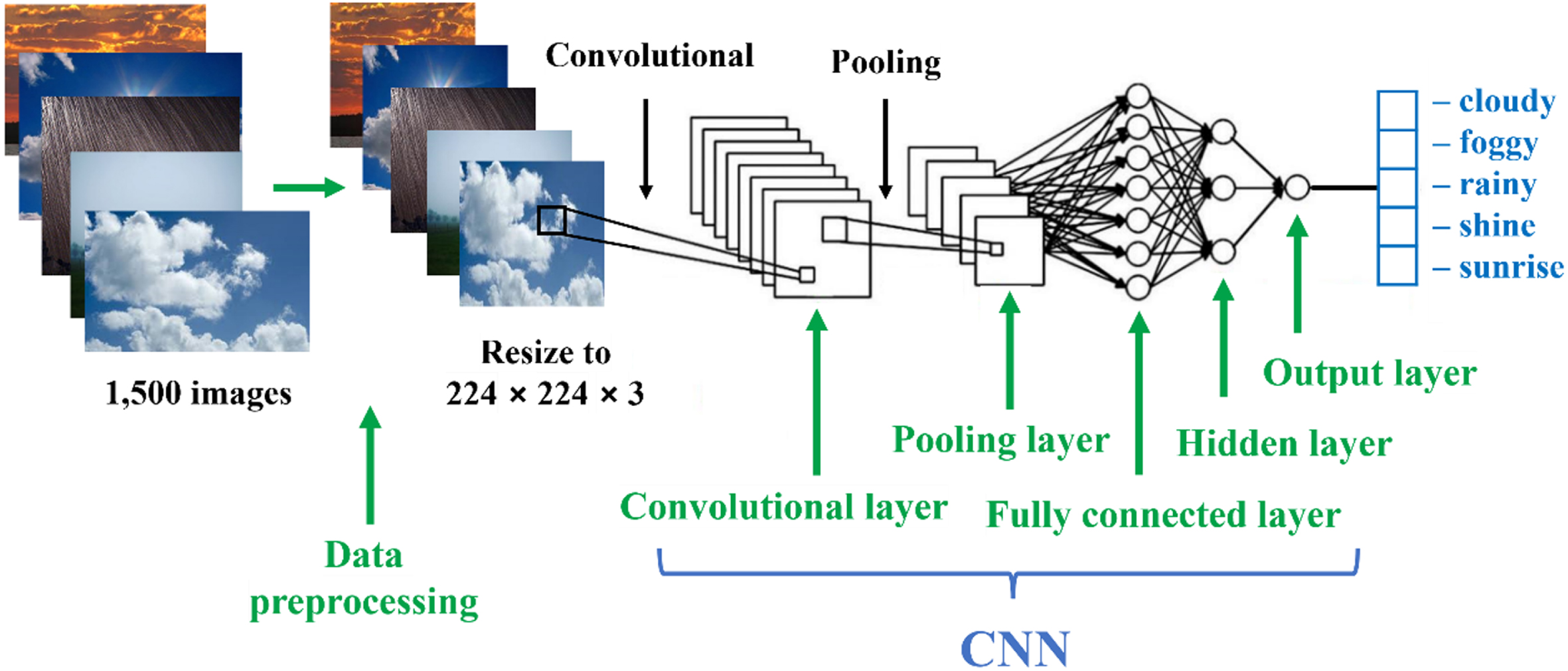
Weather image classification by CNN deep learning. A set of 1,500 image data, containing cloudy, foggy, rainy, shine, and sunrise weather type in different sizes are resized to 224×224×3 pixels with convolutional and pooling operations for the input.

In a CNN, padding is used to increase the number of rows or columns of pixels in the input image. Zero-padding is the most common padding method. In this method, the image is expanded by adding zero-value pixels around the image’s boundary. The kernel stride controls the kernel’s movement over the image’s columns and rows during convolution. The size of the output feature map can be expressed as O_f × O_f, with the following equation being valid: $O_{f} = (n + 2 p k) / s + 1$ (1) where n is the dimension of the n×n input images, k is the dimension of the k×k kernel, p is the padding, and s is the kernel stride. Kernels typically have odd height and width values because selecting a kernel with odd size and zero-padding can better preserve the spatial dimensionality of the input image. The convolution operation is intended to reduce the required computational power and achieve high-level feature extraction. An image’s color, edge, and gradient orientation are often defined as low-level features and are conventionally captured in the first convolutional layer. High-level features comprise low-level features that are captured by adding additional convolutional layers.

Pooling layers, which combine the output of clusters in one layer into the input of a single neuron in the next layer, can decrease the computational load and data dimensionality. Max pooling and average pooling are common local pooling methods in which the maximum and average value, respectively, of each input cluster is used for pooling. In general, max pooling is superior for retaining the most intense features, texture characteristics, feature selection, and classification; average pooling is more effective for dimensionality reduction and as a noise-suppression mechanism. Each kernel in the convolutional layer processes data only for its receptive field. The primary operation of a convolutional layer is to apply the kernel repeatedly to the values of the pixels from the input image. A CNN takes images as input and acquires key numerical data to identify unique image characteristics for classification. The method proposed in this paper is aimed at identifying weather events correctly for classification to enable pilots to make correct decisions to avoid potential catastrophes.

Deep-learning-based weather image classification is illustrated in Fig. 1. Image data are preprocessed by rescaling their height and width before they are input to a CNN. The chart for deep learning is shown in Fig. 2. The first is to collect image dataset. Before input to the CNN model, the raw images are to be preprocessed and split into training data and testing data. Then the CNN model will be trained by the training data, validated by the validation data and tested by the testing data. In this study, the original weather images had different sizes but were resized to a size of 224 pixels×224 pixels×3 planes for the RGB channels. Each pixel comprised 8 bits and had Huffman encoding. A set of 1500 images labeled with one of five weather types, namely cloudy, foggy, rainy, clear, and sunrise, was used for supervised learning. An example image for each category is shown in Fig. 3. The training, validation, and testing data sets were randomly selected as 70%, 10%, and 20%, respectively, of the 1500 images. The training data were used to train the proposed model, the validation data was used to evaluate the model performance during training on images that were not in the training set, and the testing data were used for the final prediction and evaluation.

Fig. 2

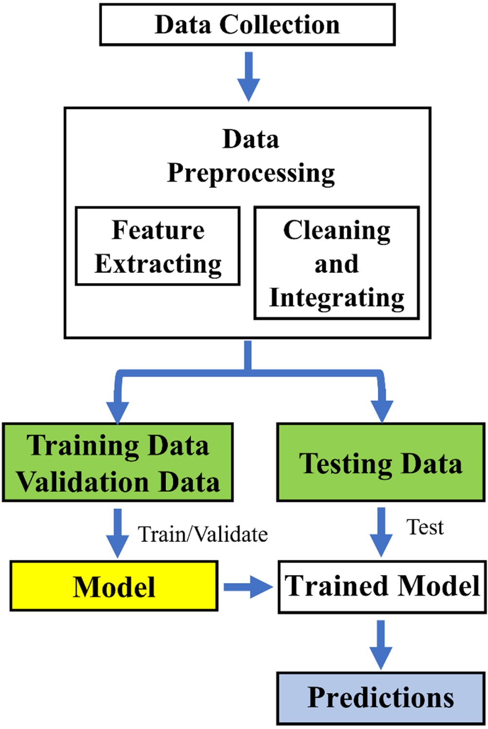
The chart of weather forecasting in deep learning. The first is to collect an image dataset. Before input into the CNN model, the raw images have to be preprocessed and split into training data, validation data and testing data. Then the model will be trained by the training data, validated by the validation data and tested by the testing data.

Fig. 3

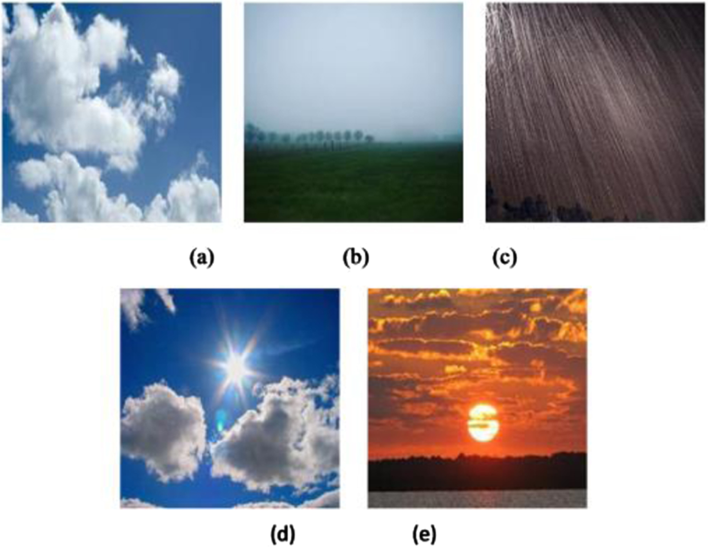
Image example of (a) cloudy, (b) foggy, (c) rainy, (d) shine, and (e) sunrise weather after resizing for CNN.

The CNN in the proposed model applies ResNet [29] for image classification, and the results of the CNN are then input to the LSTM network. The residual block in Fig. 4 is a block with a stack of two convolutional layers; the core is a skip connection. Without the skip connection, the input X would be multiplied by the layer weights. The desired underlying mapping is denoted as H(X), and the nonlinear layers (which use the rectified linear unit function) produce another mapping, namely the residual, as follows: $F (X) = H (X) - - X .$ (2)

The skip connection is used to recast the output of the original mapping to F (X) + X; thus, the model can learn more features in greater detail through its residual blocks. Skip connections improve neural network performance because they solve accuracy and saturation problems in the residual blocks, thereby reducing the difficulty of training very deep neural networks [29].

Fig. 4

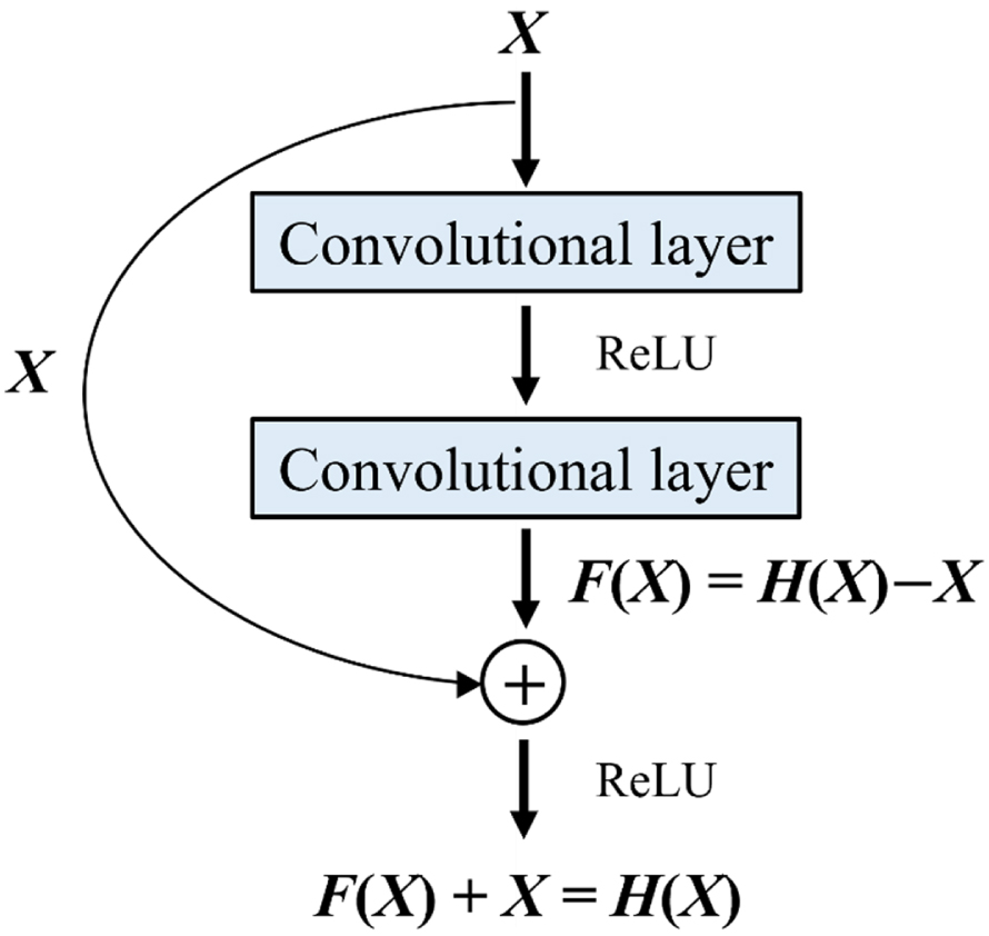
The residual block with a stack of two convolutional layers, where X is the input, H(X) is the desired underlying mapping, F(X) is another mapping that fits the nonlinear layers (ReLU) called residual, and ReLU is the activation function that allows the model to learn more nonlinear and complex functions.

Fig. 5

The training progress of the CNN in deep learning. (a) The classification accuracy in training and validation on the entire data, and (b) Training and validation loss.

Table 1

Sixteen different combinations for initial learning rate (ILR), epoch, mini-batch size (MBS) and validation frequency (VF) to the CNN performance

	Training time	ILR	Epoch	MBS	VF	Training accuracy (%)	Training loss	Validation accuracy (%)	Validation loss
1	10^′ 48^′′	0.01	5	10	10	80.00	0.51	76.00	0.63
2	10^′ 26^′′	0.001	5	10	10	100.00	0.01	94.67	0.19
3	19^′ 21^′′	0.01	10	10	10	60.00	0.67	74.00	0.63
4	19^′ 24^′′	0.001	10	10	10	100.00	0.05	96.00	0.16
5	7^′ 40^′′	0.01	5	32	10	96.88	0.13	93.33	0.26
6	7^′ 37^′′	0.001	5	32	10	100.00	0.04	97.33	0.18
7	14^′ 08^′′	0.01	10	32	10	93.75	0.19	94.67	0.25
8	14^′ 04^′′	0.001	10	32	10	100.00	0.03	94.67	0.20
9	9^′ 13^′′	0.01	5	10	30	90.00	0.24	84.67	0.55
10	9^′ 00^′′	0.001	5	10	30	100.00	0.01	94.67	0.24
11	16^′ 37^′′	0.01	10	10	30	90.00	0.22	88.67	0.44
12	16^′ 26^′′	0.001	10	10	30	100.00	0.01	94.67	0.20
13	7^′ 07^′′	0.01	5	32	30	100.00	0.03	94.67	0.21
14	7^′ 11^′′	0.001	5	32	30	100.00	0.01	96.00	0.19
15	12^′ 59^′′	0.01	10	32	30	100.00	0.04	92.00	0.52
16	12^′ 57^′′	0.001	10	32	30	100.00	0.01	97.33	0.06

Table 1 shows sixteen trials of different combinations for initial learning rate (ILR), epoch, mini-batch size (MBS) and validation frequency (VF). Each option is tested by two parameters. Compared with training time, training accuracy, training loss, validation accuracy and validation loss, the stochastic gradient descent with momentum algorithm was used with an initial learning rate of 0.001 per epoch, a maximum number of training epochs of 10, a minibatch size of 32, and a validation frequency of 30 iterations. Figure 5(a) presents the model accuracy for the training and validation data sets. The results reveal no overfitting between the training and validation data. An overfit model is overly specific to the training data and thus difficult to generalize to novel inputs. The accuracy on the validation data set was high (97.33%). During the training iterations, the accuracy was initially low but then increased quickly. After 30 iterations, the accuracy fluctuated at a high level, and after 100 iterations, the accuracy reached a limit of approximately 97%. The loss for the training data and the validation data are also shown in Fig. 5(b). The loss function for classification is the cross-entropy loss, which is defined as follows: $Loss = - \frac{1}{N} \sum_{n = 1}^{N} \sum_{i = 1}^{K} w_{i} t_{ni} \ln (y_{ni})$ (3) where N is the number of data items (N = 1050 for the training data and 150 for the validation data), K = 5 is the number of categories, w_i is the weight for category i, t_ni is a binary indicator (0 or 1) of whether datum n belongs to category i, and y_ni is the output for datum n and category i. The loss was initially high (2.41) and then quickly decreased to 0.23; it stabilized at approximately 0.09 after 100 iterations.

The confusion matrix is often adopted to evaluate the precision, false discovery ∼ rate, sensitivity, false positive rate, and overall accuracy of predictive models, such as deep learning models. The confusion matrix of the proposed model is depicted in Fig. 6. The diagonal and off-diagonal entries indicate the number of correct and incorrect classifications, respectively, of input images from the testing data. For example, the first column represents the model’s performance for predicting the “cloudy” category from the testing data. From the top to the bottom of the column, 58 images were correctly classified as cloudy; 2 were misclassified as clear; and none were classified as foggy, rainy, or sunrise. The upper number of the right column represents the precision, and the bottom number represents false the discovery rate. The upper number of the bottom row is the sensitivity, the bottom number is the false positive rate, and the lower-right number is the overall accuracy. For example, the upper-right corner indicates that 59 images in the testing data were classified as cloudy; 58 images were correctly classified, and only one image was misclassified. Therefore, the model precision for the cloudy category was 98.31%, and the false discovery rate was 1.69%. The data in the bottom-left corner reveal that, of all the cloudy images in the testing data, 58 images were correctly classified, and two images were misclassified; therefore, the model sensitivity for the cloudy category was 96.67%, and the false positive rate was 3.34%. The lower-right data indicate the overall accuracy of the weather forecasting model. The proposed model had an overall accuracy of 97.67% for the classification of the five categories of weather images (Fig. 6).

Fig. 6

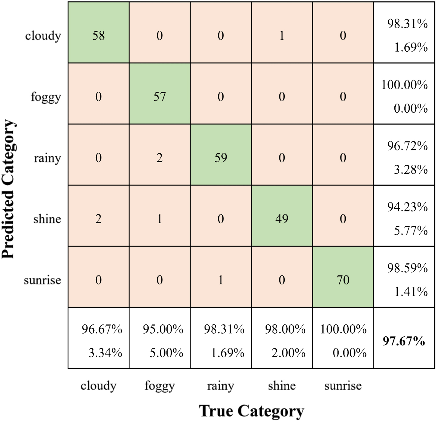
The confusion matrix showing the performance of CNN in predictive analytics, where the diagonal are correct classification and the off-diagonal are otherwise. The last column and the last row are the true/false rate.

3 Long short-term memory

In aviation safety, though CNN can identify and classify the incoming weather, it cannot quantify nor predict numerical information. The multivariate numerical forecasting by LSTM in deep learning is shown in Fig. 7. An LSTM composed of three gates with feedback connection. The gates update and control the cell states C_t and the hidden states h_t. The cell state C_t is to model long-term memory that stores the information of previous time step and encodes data aggregation from the previous time step. The hidden state h_t is to model short-term memory by encoding recent time step data. LSTM utilizes the three gates, the forget gate f_t, input gate i_t and output gate o_t with sigmoid (σ) and tanh activation functions, to compensate what RNN lacks in memorizing and forgetting the input x_t, where the sigmoid function is to calculate a set of scalars for preventing vanishing/exploding gradients and the tanh function is to normalize the data.

Fig. 7

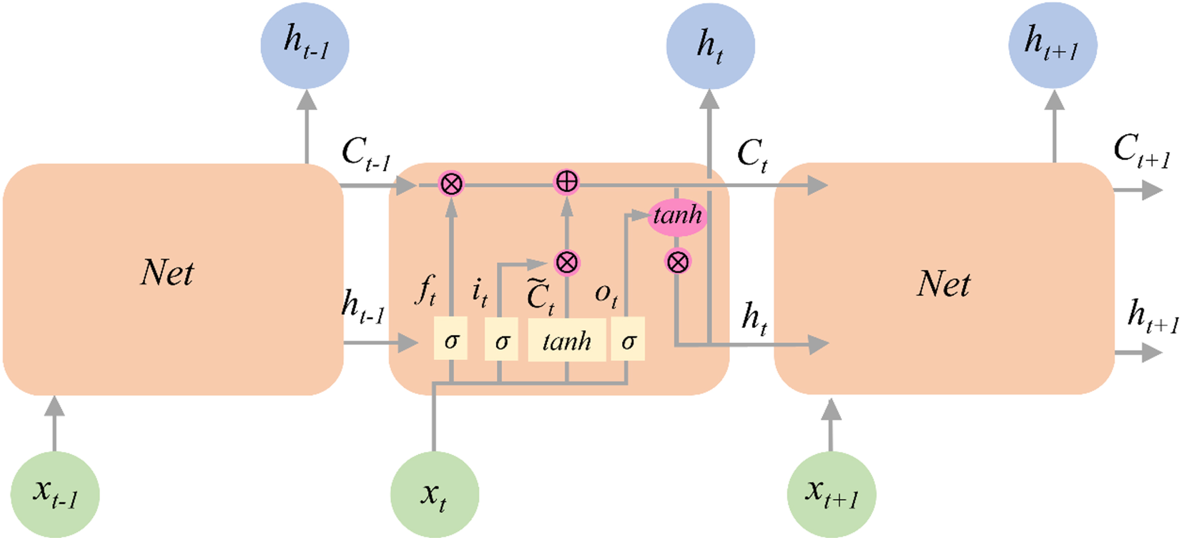
An LSTM contains four interacting layers by feedback connection, where ⊗ is the pointwise multiplication, ⊕ is the pointwise addition, σ is the sigmoid function, f_t is the forget gate, i_t is the input gate, o_t is the output gate and ${\tilde{C}}_{t}$ is the cell state at present time step. The subscript t - 1, t, and t + 1 are the previous, present, and next time step, respectively.

The forget gate f_t is to decide if the output of the previous time step and the input at present time step should be kept or not, $f_{t} = σ [(w_{f} (h_{t - 1} + x_{t}) + b_{f}]$ (4) where w_f and b_f are the weight and offset of the forget gate and h_t-1 is the hidden state of the previous time step. The input gate i_t is to quantify the importance of input, where a new candidate cell state ${\tilde{C}}_{t}$ is to control the information to be encoded, $i_{t} = σ [(w_{i} (h_{t - 1} + x_{t}) + b_{i}]$ (5) ${\tilde{C}}_{t} = tanh [(w_{c} (h_{t - 1} + x_{t}) + b_{c}]$ (6) where w_i and b_i are the weight and offset of the input gate i_t, and w_c and b_c are the weight and offset of the new candidate cell state ${\tilde{C}}_{t}$ .

The new cell state C_t is updated by multiplying the previous cell state C_t-1 with the forget gate f_t and adding a new candidate of cell state $i_{t} * {\tilde{C}}_{t}$ , where * denotes convolution operation, $C_{t} = f_{t} * C_{t - 1} + i_{t} * {\tilde{C}}_{t}$ (7)

The output gate o_t is to control the number of input to the next time step by encoding or filtering the information, $o_{t} = σ [(w_{o} (h_{t - 1} + x_{t}) + b_{o}]$ (8) $h_{t} = o_{t} * tanh (C_{t})$ (9) where w_o and b_o are the weight and offset of the output gate, h_t is the output of hidden state representing short-term memory and C_t is the cell state representing long-term memory. These three gates allow having knowledge about the cell state and hidden state at every time step to address the vanishing gradient problem. Therefore, LSTM is often used to train long time series data such as weather forecasting.

For the LSTM shown in Fig. 8, a sequence input layer is applied with 500 hidden units for output, a fully connected layer is then used to map the desired output, and the regression output layer is to compute the mean square error loss. The initial learning rate is to control how much to change the model in response to the estimated error each time the model w is updated. One epoch is when an entire data is passed forward and backward through the neural network only once. The learning rate schedule is to drop the learning rate during training, “none” means the learning rate remains constant throughout the training, and “piecewise” means the software updates the learning rate every certain number of epochs by multiplying with a certain learning rate factor. The learning rate drop factor is a factor to drop the learning rate, specified as a scalar from 0 to 1 to apply to the learning rate every time a certain number of epochs passes. The gradient threshold is set as a positive value. If the gradient exceeds the value of the gradient threshold, then the gradient is clipped to help prevent gradient explosion by stabilizing the training at higher learning rates and in the presence of outliers. For setting the training cycle, the initial learning rate factor is 0.005, the maximum number of training epochs is 250, the learning rate schedule is set to “piecewise”, the learning rate drop factor is 0.2, and the gradient threshold is 1. After training, a figure of training progress is to check overfitting. The testing data are then applied to the LSTM. 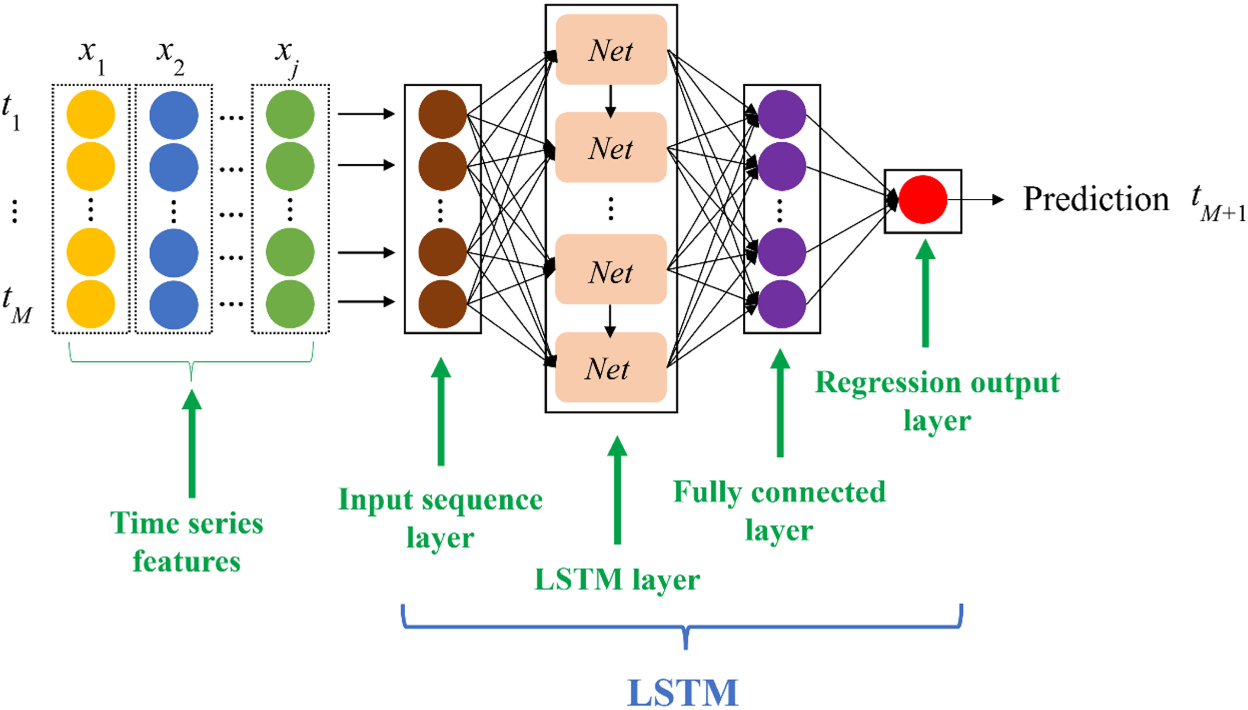Data preprocessed in z-score standardization is adopted by $x^{'} = (x - μ) / β$ (10) where x is the original data, x′ is the new data after preprocessing, μ is the mean value of the data, and β is the standard deviation.

Fig. 8

The numerical forecasting by LSTM deep learning, which is composed of an input sequence layer, the LSTM layer, fully connected layer and regression output layer. A time series of weather features is the input, where t is the time step, j is the number of features, M is the number of observations of the features and Net is the LSTM neural network.

Visibility is more difficult to predict than other weather factors such as temperature and humidity. Prolonged low-visibility weather will cause extensive airport delays and cancellations. Zhu et al. [30] used deep learning to show that the multi-factor prediction model was more stable than the single factor in airport visibility prediction. Zhang et al. [28] proposed multimodal fusion to predict weather visibility by fusing numerical prediction with satellite image for improving visibility prediction. It is necessary to know the visibility when temperature and humidity are reduced to critical points causing aircraft icing before entering into dense fog.

In this study, visibility forecasting is trained by eleven years of weather data from 2010 to 2020. The data contain 10 weather information: sea pressure (SP), temperature (T), dew point temperature (DP), relative humidity (RH), wind speed (WS), wind direction (WD), sunshine rate (SR), global solar radiation (GR), visible mean (VM) and cloud amount (CA). The testing data is divided into 36 days and the remaining data is the training data. When processing a time series problem with an LSTM in deep learning, the root mean square error (RMSE), the mean square error loss and the mean absolute percentage error (MAPE) are often used as performance indicators $RMSE = {(\frac{1}{M} \sum_{i = 1}^{M} {(y_{i} - \hat{y_{i}})}^{2})}^{1 / 2}$ (11) $Loss = \sum_{i = 1}^{M} {(y_{i} - \hat{y_{i}})}^{2} / M$ (12) $MAPE = \frac{1}{M} \sum_{i = 1}^{M} | (y_{i} - \hat{y_{i}}) / y_{i} |$ (13) where M is the number of observed data, y_i is the real value, and $\hat{y_{i}}$ is the forecast value. The mean square error loss represents the difference between the real and forecast values which are extracted by squaring the average difference over the data. It is a measure of how close a fitted line is to the actual value. RMSE is the error rate by the square root of mean square error loss. It is often used when assessing how well a model fits the data because it is measured in the same units as the forecast value. MAPE is a measure of forecasting accuracy and it is also commonly used in regression problems because of intuitive interpretation in terms of relative error. If the MAPE is lower than 10%, the forecast highly accurate; between 10% to 20%, good; between 20% to 50%, reasonable; and higher than 50%, weak and inaccurate. The RMSE of using the remaining 9 features of eleven years data to predict the visibility is 12.02, and the MAPE is 44.46%. To select sensitive predictor features to increase visibility forecasting is necessary.

The process of feature selection goes through the multiple linear regression first and then the Pearson’s correlation coefficient. Multiple linear regression is used to select sensitive predictor features by describing the relationship between a dependent variable and one or more independent variables. The dependent variable y is also called the response feature and the independent variables x are also called predictor features. The multiple linear regression used in this study is $\begin{matrix} y_{i} = α_{0} + α_{1} x_{i 1} + α_{2} x_{i 2} + \dots \\ + α_{j} x_{ij} + ɛ_{i} i = 1, \dots, M \end{matrix}$ (14) where y_i is the i response, α_j is the j correlation coefficient, j is the amount of predictor features, x_ij is the i observation on the j predictor feature, and ɛ_i is the i random error. The correlation coefficient of the regression line describes the mathematical relationship between each independent variable and the dependent variable, and the p-values for the correlation coefficients indicate whether these relationships are statistically significant. The significance level is the probability of rejecting the null hypothesis when it is true and often set at 0.05. The result of the multiple linear regression is shown in Table 2. SR and CA are the predictor features whose p-value are greater than 0.05 and will be deleted. Table 4 shows that selecting sensitive features by multiple linear regression can reduce the RMSE and MAPE from 12.02 to 11.91 and 44.46% to 39.02%, respectively. It is necessary to keep selecting more sensitive features to enhance the forecast accuracy.

Table 2

The p-value of response feature visibility and predictor feature by multiple linear regression

SP	T	DP	RH	WS	WD	SR	GR	CA
0.000	0.000	0.000	0.000	0.000	0.006	0.106	0.000	0.140

Table 3

Pearson’s correlation coefficient matrix for the linear relationship between the response feature and predictor features^*

Feature	SP	T	DP	RH	WS	WD	GR	VM
SP	1.00	–0.84	–0.85	0.10	0.29	–0.34	–0.43	–0.18
T	–0.84	1.00	0.92	–0.32	–0.27	0.31	0.66	0.37
DP	–0.85	0.92	1.00	0.07	–0.30	0.28	0.42	0.20
RH	0.10	–0.32	0.07	1.00	–0.05	–0.09	–0.63	–0.44
WS	0.29	–0.27	–0.30	–0.05	1.00	–0.50	–0.10	0.09
WD	–0.34	0.31	0.28	–0.09	–0.50	1.00	0.21	0.03
GR	–0.43	0.66	0.42	–0.63	–0.10	0.21	1.00	0.51
VM	–0.18	0.37	0.20	–0.44	0.09	0.03	0.51	1.00

^*SP: sea pressure, T: temperature, DP: dew point temperature, RH: relative humidity, WS: wind speed, WD: wind direction, SR: sunshine rate, GR: global solar radiation, CA: cloud amount, VM: visible mean.

Table 4

The RMSE and MAPE of visibility forecasting by different predictor feature combinations

Data description	Predictor feature combinations	Deleted predictor feature	RMSE	MAPE(%)
–	All	–	12.02	44.46
with multiple linear regression	SP+T+DP+RH+WS+WD+GR	SR, CA	11.91	39.02
with multiple linear regression and the Pearson’s correlation coefficient	T+RH+GR	SP, DP, WS, WD, SR, CA	10.12	36.77
with CNN integration	T+RH+GR+VL	SP, DP, WS, WD, SR, CA	2.68	13.41

The Pearson’s correlation coefficient (ρ) of two features (e.g., x_A and x_B) is a measure of their linear dependence and defined as ${ρ (x}_{A} {, x}_{B}) = \frac{1}{M - 1} \sum_{i = 1}^{M} (\frac{x_{Ai} - μ_{A}}{β_{A}}) (\frac{x_{Bi} - μ_{B}}{β_{B}})$ (15) where μ_A and β_A are the mean and standard deviation of feature x_A, respectively, and μ_B and β_B are the mean and standard deviation of feature x_B. If 0 . 1 < |ρ| < 0 . 3, the two features are of low intensity; 0 . 3 < |ρ| < 0 . 5, medium intensity; and 0 . 5 < |ρ| < 1 . 0, high intensity. The Pearson’s correlation coefficient matrix of SP, T, DP, RH, WS, WD, GR and VM is shown in Table 3. The result shows that the intensity between visibility and other features from the highest to the lowest is GR, RH, T, DP, SP, WS and WD in order. Most of the coefficients are low and medium. GR is the only predictor feature with high intensity, but its coefficient of 0.51 is close to moderate intensity. Deleting DP, SP, WS and WD with low intensity, the remaining features GR, RH and T are for LSTM training. Table 4 shows that selecting sensitive features by multiple linear regression and the Pearson’s correlation coefficient can further reduce the RMSE and MAPE to 10.12 and 36.77%, respectively. The collected data often come in enormous quantities and some of the features might not contribute significantly to the performance of the model. Selecting sensitive features by multiple linear regression and the Pearson’s correlation coefficient can speed up the training process without redundant features and lead the model to learn from relevant features and increase forecast accuracy.

In this section, the result shows that data preprocessing can improve training convergence and accuracy. In addition, the number of data should be considered if there is still no effect on the prediction when the data has been preprocessed, especially for the feature that has a less interrelated correlation with others. Using linear regression and Pearson’s correlation coefficients as feature selection methods, and adding an additional visibility level feature, the proposed LSTM model can improve visibility forecasting.

4 Integration of CNN and LSTM

Aviation visibility is considered more difficult to predict because there is no highly interrelated correlation between visibility and any predictor feature. Deleting the predictor features of low relation coefficient (low intensity) only reduces the RMSE from 11.91 to 10.12 and MAPE from 39.02% to 36.77%. This study proposes to integrate CNN and LSTM as shown in Fig. 8 so as to increase forecast accuracy. CNN in Fig. 9 will first classify different weather images, then the classification will be considered a feature fused to the numerical data in LSTM visibility forecast. The added feature is replaced by classifying the numerical data of visibility into six visibility levels (VL) for every 10 km due to the unavailability of associated weather image data in this study. Level 1 is for 0– 10 km, level 2 for 11– 20 km, level 3 for 21– 30 km, level 4 for 31– 40 km, level 5 for 41– 50 km and level 6 for 51– 60 km. The VL is training with the sensitive features, T, RH and GR, selected by multiple linear regression and the Pearson’s correlation coefficient for LSTM prediction in Fig. 8. The result shows that visibility forecasting has a significant improvement in decreasing RMSE from 10.12 to 2.68 and MAPE from 36.77% to 13.41% in Table 4. The forecast results of visibility with different combinations are shown in Fig. 10(a). After deleting the least sensitive predictor feature and adding VL, the best predictor feature combination for the visibility forecasting is T, RH, GR and VL, and Fig. 10(b) shows the error of the visibility forecast and the observed value, respectively. Integrating CNN and LSTM has the lowest forecast error approximate 2.54 km than others. In addition, using linear regression and Pearson’s correlation coefficients as feature selection methods, and adding an additional visibility level feature, the proposed LSTM model can improve visibility forecasting. The estimated visibility forecast errors are small compared to the research of RMSE 6.71 by Zhang et al. [28].

Fig. 9

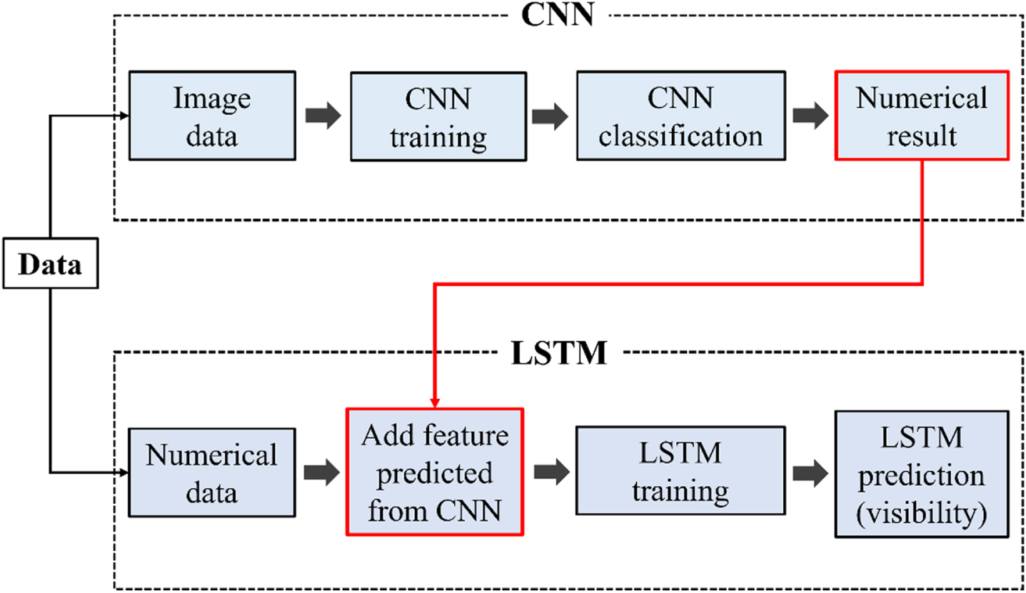
Integration of CNN and LSTM for visibility forecasting. The CNN will first classify different weather image data, then a feature will be added to the numerical data by transforming the CNN classification result into numerical result for LSTM training.

Fig. 10

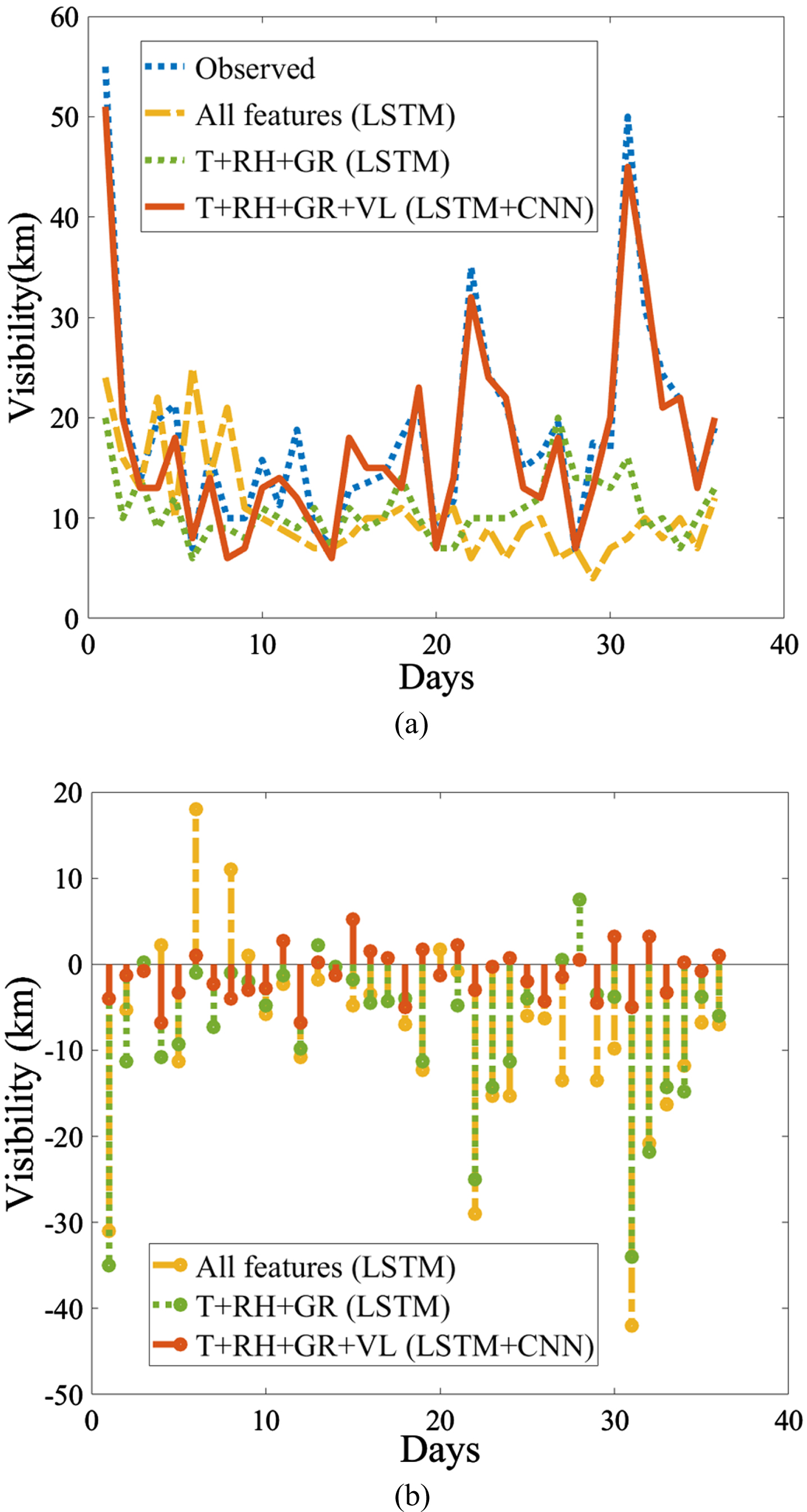
Visibility forecasting by LSTM with different feature combinations, (a) the best combination is T + RH+SR+VL (LSTM+CNN) and (b) RMSE 2.68 and MAPE 13.41%.

As a result, if the associated weather image of the numerical data in this study can be obtained simultaneously, the label of the weather images can be transformed into visibility levels in a CNN to improve the forecast of visibility by representing an additional predictor feature rather than manually creating it. Each category can be rated for the weather conditions on a scale of number. For instance, “shine” refers to good weather that has a high visibility, so it will be labeled into scale of the largest number, in other words, “foggy” will be labeled into scale of the smallest number because of its low visibility. The visibility forecast by integrating CNN result as precursor to LSTM is shown effective to enhance aviation safety with the characteristics utilization in deep learning.

5 Conclusions

Conventionally, forecasters can only make subjective forecasts based on their experience in the absence of forecasting tools. Forecast quality is often limited by the forecaster’s understanding of regional characteristics and the influence of past experience, for which maintaining stable and accurate levels is difficult. An integration of CNN and LSTM is proposed to increase the visibility forecast accuracy. The CNN will first train and classify different weather image data, then a feature will be added to the numerical data by transforming the CNN classification result into numerical result of relative visibility level (VL) for LSTM training. Compared to the numerical weather prediction (NWP), the weather forecast generated by deep learning is more efficient with better accuracy.

A dataset of 1500 weather images was preprocessed, resized, and input into a CNN for training. The training, validation, and testing accuracy were 100.00%, 97.33%, and 97.67%, respectively. These results reveal that a CNN can classify weather images. To process numerical data, an LSTM network was developed, and the Pearson correlation coefficients and multiple linear regression were integrated into the feature selection methods to select sensitive features related to the visibility. The results indicate that temperature, relative humidity, and global solar radiation are sensitive features. When using these features, the root mean square error (RMSE) and mean absolute percentage error (MAPE) of the proposed model decreased 12.02 to 10.12 and from 44.46% to 36.77%, respectively.

Atmospheric visibility is difficult to predict. However, the results of this study indicate an integrated CNN– LSTM network model can achieve high accuracy in atmospheric visibility prediction. The inclusion of the visibility level in the sensitive features selected during feature selection caused the RMSE and MAPE to decrease from 10.12 to 2.68 and from 36.77% to 13.41%, respectively. The estimated visibility forecast errors are small compared to the research of RMSE 6.71 by Zhang et al. [28]. If numerical data and the associated weather images can be obtained simultaneously, the visibility forecasting performance of the proposed model can be further improved. Moreover, the behavior of a deep learning network on numerical weather data for aviation can be explored using the proposed model.

This paper presents an integrated model combining CNN and LSTM for aviation visibility forecasting. By utilizing the feature extraction capability of CNN and the temporal learning ability of LSTM, the model takes historical meteorological images and data as input and predicts visibility values for future time periods. Compared to NWP methods, the proposed approach offers several advantages. It does not rely on complex physical models, can handle nonlinear and non-stationary relationships, and demonstrates higher accuracy and generalization ability. However, there are also some limitations to the proposed method. It necessitates a substantial amount of historical data for training the model, which may not always be available or reliable. Additionally, it is a black-box model that poses challenges in terms of interpretation and justification in practical applications. Furthermore, the method involves multiple hyperparameters that require careful tuning, but a systematic approach to finding the optimal settings is lacking.

Although the method has better prediction effect, the detailed analysis of its forecast results also found some shortcomings, such as predictive visibility turn or turn bad times have a certain lag. In addition, we will cooperate with low weather conditions, and try to combine the ability to reflect low-level stratification conditions, high-altitude wind field and ground pressure field and other factors as a forecasting factor to ensure that the forecasting factor can better contain the low visibility weather conditions to improve the prediction effect of the model. Next, we will try to incorporate this model into real applications and conduct continuous testing to improve the quantitative forecasting capacity of this methodology.

Footnotes

Acknowledgments

This work was supported in part by the National Science and Technology Council, Taiwan, ROC under contract NSTC 111-2410-H-309-001-. The author is grateful to the reviewers and AE for their exceptional efforts in enhancing the style and clarity of this paper.

Data availability

The input weather information is collected from the database: .

Declaration of interest statement

The authors declared that they have no conflicts of interest in this work.

References

Wang

, Zheng

, Li

, Xu

, Liu

and Zhang

, Tropical cyclone intensity estimation from geostationary satellite imagery using deep convolutional neural networks, IEEE Transactions on Geoscience and Remote Sensing 60 (2021), 1–16.

Ren

, Li

, Ren

, Song

, Xu

, Deng

and Wang

, Deep learning-based weather prediction: a survey, Big Data Research 23 (2021), 100178.

Yuan

, Wang

, Mu

, Zhou

and Duan

, Typhoon intensity forecasting based on LSTM using the rolling forecast method, Algorithms 14(3) (2021), 83.

Chen

, Kuang

, Wang

, Chen

, Han

and Fan

, Storm surge prediction based on long short-term memory neural network in the East China Sea, Applied Sciences 12(1) (2021), 181.

Wei

C.C.

, Collapse warning system using LSTM neural networks for construction disaster prevention in extreme wind weather, Journal of Civil Engineering and Management 27(4) (2021), 230–245.

Caseri

A.N.

, Santos

L.B.L.

and Stephany

, A convolutional recurrent neural network for strong convective rainfall nowcasting using weather radar data in southeastern brazil, Artificial Intelligence in Geosciences 3 (2022), 8–13.

Ren

, Xu

and Cui

, Typhoon track prediction based on deep learning, Applied Sciences 12(16) (2022), 8028.

Zhou

, Xu

, Qian

, Xu

and Xu

, Discriminating technique of typhoon rapid intensification trend based on artificial intelligence, Atmosphere 13(3) (2022), 448.

Tao

, Awadh

S.M.

, Salih

S.Q.

, Shafik

S.S.

and Yaseen

Z.M.

, Integration of extreme gradient boosting feature selection approach with machine learning models: application of weather relative humidity prediction, Neural Computing and Applications 34(1) (2022), 515–533.

10.

Maqsood

, Khan

M.R.

and Abraham

, Intelligent weather monitoring systems using connectionist models, Neural, Parallel & Scientific Computations 10(2) (2002), 157–178.

11.

Maqsood

, Khan

M.R.

and Abraham

, Weather forecasting models using ensembles of neural networks, Intelligent Systems Design and Applications, Germany (2003), 33–42.

12.

Paras

S.M.

, Kumar

and Chandra

, Feature based neural network model for weather forecasting, International Journal of Computational Intelligence Systems 4(3) (2008), 209–216.

13.

Reichstein

, Camps-Valls

, Stevens

, Jung

, Denzler

and Carvalhais

, Deep learning and process understanding for data-driven earth system science, Nature 566 (2019), 195–204.

14.

Akdi

and Ünlü

K.D.

, Periodicity in precipitation and temperature for monthly data of Turkey, Theoretical and Applied Climatology 143 (2021), 957–968.

15.

Akbal

and Ünlü

K.D.

, A deep learning approach to model daily particular matter of Ankara: key features and forecasting, International Journal of Environmental Science and Technology, 19 (2022), 5911–5927.

16.

M.W.

, Xu

D.Y.

, Geng

and Hong

W.C.

, A hybrid approach for forecasting ship motion using CNN-GRU-AM and GCWOA, Applied Soft Computing 114 (2002), 108084.

17.

, Zhang

and Krebs

, Prediction of flow based on a CNN-LSTM combined deep learning approach, Water 14(6) (2022), 993.

18.

Ravuri

, Lenc

, Willson

, Kangin

, Lam

, Mirowski

, Fitzsimons

, Athanassiadou

, Kashem

, Madge

, Prudde

, Mandhane

, Clark

, Brock

, Simonyan

, Hadsell

, Robinson

, Clancy

, Arribas

and Mohamed

, Skilful precipitation nowcasting using deep generative models of radar, Nature 597 (2021), 672–677.

19.

Zhao

, Li

, Lu

and Wang

, A CNN-RNN architecture for multi-label weather recognition, Neurocomputing 322 (2018), 47–57.

20.

Weyn

J.A.

, Durran

D.R.

and Caruana

, Improving data-driven global weather prediction using deep convolutional neural networks on a cubed sphere, Journal of Advances in Modeling Earth Systems 12(9) (2020). doi,org/10.1029/2020MS002109

21.

Denby

, Discovering the importance of mesoscale cloud organization through unsupervised classification, Geophysical Research Letters 47(1) (2020).

22.

Tan

, Xuan

, Xia

and Wang

, Weather recognition based on 3C-CNN, KSII Transactions on Internet and Information Systems 14(8) (2020), 3567–3582.

23.

Liu

, Racah

, Correa

, Khosrowshahi

, Lavers

, Kunkel

, Collins

and Wehner

, Application of deep convolutional neural networks for detecting extreme weather in climate datasets, Computer Vision and Pattern Recognition, (2016). doi,org/10.48550/arXiv,1605.01156.

24.

Heinzler

, Piewak

, Schindler

and Stork

, CNN-based lidar point cloud de-noising in adverse weather, IEEE Robotics and Automation Letters 5(2) (2020), 2514–2521.

25.

Zhou

, Zheng

, Li

, Dong

and Zhang

, Forecasting different types of convective weather: a deep learning approach, Journal of Meteorological Research 33(5) (2019), 797–809.

26.

Weyn

J.A.

, Durran

D.R.

and Caruana

, Can machines learn to predict weather? using deep learning to predict gridded 500-hPa geopotential height from historical weather data, Journal of Advances in Modeling Earth Systems 11(8) (2019), 2680–2693.

27.

Elhoseiny

, Huang

and Elgammal

, Weather classification with deep convolutional neural networks, IEEE-International Conference on Image Processing, (2015), 3349–3353.

28.

Zhang

, Wu

, Chen

, Zhang

, Xie

, Huang

and He

, Weather visibility prediction based on multimodal fusion, IEEE Access 7 (2019), 74776–74786.

29.

, Zhang

, Ren

and Sun

, Deep residual learning for image recognition, IEEE Conference on Computer Vision and Pattern Recognition, (2016), 770–778.

30.

Zhu

, Zhu

, Han

and Wang

, The application of deep learning in airport visibility forecast, Atmospheric and Climate Sciences 7(3) (2017), 314–322.