Features reduction collaborative fuzzy clustering for hyperspectral remote sensing images analysis

Abstract

In image processing, segmentation is a fundamental problem but an important step for advanced image processing problems. When dealing with hyperspectral image data, the task becomes much more challenging due to the large number of features (dimension), higher nonlinearity, and greater capacity of the data. This paper proposes a solution of features reduction collaborative fuzzy c-means clustering (FR-CFCM) for hyperspectral remote sensing image analysis using random projection. The dimensional reduction technique is based on the Johnson Lindenstrauss lemma algorithm, preserving the relative distance between data samples. This can make clustering easier without affecting the clustering results. Moreover, by reducing dimensionality and sharing information among sub-data in collaborative clustering, it is possible to improve the performance and accuracy of hyperspectral remote sensing image analysis results. The experiments conducted on two hyperspectral image data sets with five validity indexes show that the proposed methods perform better compared with the other methods.

Keywords

hyperspectral image fuzzy clustering collaborative clustering feature reduction

1 Introduction

Hyperspectral imaging (HSI), which acquires hundreds of individualized reflectance or fluorescence spectrum for each pixel, is applied in various fields and is one of the most comprehensive applications in earth observation [1]. HSI has huge numbers of narrow and contiguous bands that involves high computation complexity in processing and analyzing the image. Hence dimensionality reduction is applied as an essential pre-processing step for HSI data.

HSI is a technology that can accurately identify and characterize any material by measuring the radiation that reaches the sensor with high spectral resolution across a wide range of spectral bands. This allows for the differentiation of various land-cover classes such as water, soil, forestry, crops, and urban areas [2]. When analyzing images, image segmentation is a crucial but difficult step, especially when dealing with the complex task of processing HSI data [3]. There are several factors that contribute to the complexities of the situation. These include a limited number of training samples, the curse of dimensionality, the variability of hyperspectral signals across different land-cover classes, and the impacts of the atmosphere [4].

In recent years, various methods have been suggested to address the challenge of dealing with a vast number of spectral bands, which is known as the curse of dimensionality. This issue has a significant impact on hyperspectral image segmentation. In data analysis, a feature refers to an attribute or dimension that impacts the problem at hand. It is essential to select the most significant features for a model to ensure its effectiveness [5]. Reducing the dimensions of HSI can serve as a necessary preparation for segmentation, helping to eliminate unnecessary components and simplify the computational process.

Two common dimensionality reduction methods are feature selection [6, 7] and feature extraction [8]. Both feature selection and feature extraction are used for dimensionality reduction which is key to reducing model complexity and overfitting. Although feature selection and extraction processes may have the same objective, both are completely different from each other. The main difference between them is that feature selection is about selecting the subset of the original feature set, whereas feature extraction creates new features [9]. Feature selection identifies the "important features" in the high-dimensional data sets to understand the underlying phenomena of interest [10].

In contrast, feature extraction builds derived features from initial features of data sets intended to be informative and non-redundant. Most dimensionality reduction processes are based on multivariate analysis: projecting data onto a subspace that maximizes explained variance and minimizes correlation. The primary goal of dimensionality reduction techniques is to decrease the number of dimensions without losing the structural details of the data [11, 12].

Accordingly, it can be considered that principal component analysis (PCA) is a form of feature extraction algorithm, which creates new features from features. PCA is one of the most used algorithms because it is simple and fast. However, this algorithm has limitations such as only working with numeric data, being sensitive to outlier/extreme points, and not being suitable for nonlinear models, because PCA is completely based on linear transformations. In the paper [5], a new semi-supervised dimensionality reduction (DR) method, termed geodesic-based manifold joint hypergraphs (GMJHs), is proposed for HSI.

Dealing with the spectral variability and nonlinearity of HSI is a challenge for many existing classification methods [13]. To solve these problems, Feng al et. proposed a simple spectral hierarchical feature fusion and selection network (HFFSNet) [14]. Specifically, the paper applies 1-D grouped convolution for dimensionality reduction and multilevel feature extraction. The multilevel features are fused to assist the adaptive feature selection of different layer features via the soft attention mechanism, and finally, the selected features are fused to further enhance the feature representation. Extensive experimental results on HSI datasets demonstrate the effectiveness of the proposed network. In the paper [15], an unsupervised dimensionality reduction (DR) method termed Laplacian regularized collaborative representation projection (LRCRP) is proposed, where Laplacian regularization and local enhancement are introduced into collaborative representation (CR) to construct an adjacent graph and then to reduce the spectral dimension in graph embedding framework [16].

Much related work has recently been carried out to solve the HSI segmentation problems. In general, there are three approaches to HIS segmentation: the first is based on unsupervised learning techniques; the second is based on supervised learning techniques, such as support vector machine (SVM) [8, 17], and the third is based on semi-supervised learning techniques. In fact, many datasets have little or no sample data, so supervised learning algorithms cannot be applied.

Due to the lack of data samples, clustering is one of the most commonly applied techniques for segmenting images [6, 18]. Some hybrid techniques have also been proposed by many researchers and produce good results, such as using kernel methods [3, 19–21]; applying evolutionary algorithms to increase cluster accuracy [22, 23]. Moreover, most clustering algorithms use a combination of spectral information and spatial information to optimize segmentation results [24]. However, when working with data with a large number of attributes like HSI, besides accuracy, computational complexity also needs to be considered [25].

The purpose of clustering methods is to identify patterns in data sets. This helps group objects together that share similarities and are positioned within the same cluster [26, 27]. Clustering was briefly associated with data mining techniques, which include machine learning and knowledge discovery [28]. Various algorithms have been implemented for various applications and industries. Clustering methods have led to a notable improvement with regards to k-means and their advancement [29, 30] and a family of Fuzzy C-Mean (FCM) methods [31–33].

A particular type of FCM, collaborative fuzzy clustering, was developed in [34, 35] as an approach to detect a pattern and reveal similarity on many data sets [36]. The collaborative clustering technique is adopted to enhance the ability to recognize the intrinsic structure of clusters [37, 38]. In which, each cluster will adjust the clustering results against all other groups according to the collaborative parameter until all clusters are optimized [39]. With the above advantages, the collaborative fuzzy clustering method has been studied by many scientists [40]. However, there are not many studies on collaborative fuzzy clustering in hyperspectral remote sensing image data analysis problems because of their difficulties [41].

When processing HSI data, there are two main challenges to overcome: the high dimensionality of the data and the large number of instances. With the goal of HSI segmentation, we present a solution that involves reducing dimensionality through random projection. Next, the data is divided into smaller data sets, or data sites, and locally clustered. Finally, collaborative clustering is performed to complete the process. The objective of this approach is to decrease computation time while still benefiting from the advantages of the collaborative fuzzy clustering algorithm. The dimensionality reduction method in the paper is based on the Johnson Lindenstrauss lemma algorithm, which also preserves the relative distance between data samples. These can help reduce the computation time for the proposed algorithm and also improve the accuracy of the image segmentation results.

The paper is organized as follows: Section II offers a brief introduction to random projection dimensionality reduction, FCM, and collaborative clustering; Section III proposes a novel method for HSI segmentation; Section IV shows the experimental results; The conclusion and future studies are covered in Section V.

2 Background

2.1 Random projection features reduction

Formally, a dimensionality reduction technique can be defined as follows. Given a dataset of d-dimensions, we find a function such that f : R^d → R^k, with k < d. The function f projects the original d-dimensional data to k - dimensional data with the constraint k < d. Most dimensionality techniques share two common properties [42] but the ensemble of these two properties in a dimensionality reduction method would produce a state-of-the-art technique for reducing high dimensional data.

The dimensionality reduction used in this paper is a random projection. The main idea behind this random projection is from a popular lemma named Johnson Lindenstrauss (JL) lemma [43].

The lemma states: given a finite set X ⊂ R^d of size |X| = K, there exists a linear map f : R^d → R^k with k = O (ɛ^-2 * log K) such that:

(1 - ɛ) ‖ x - y ‖ ₂ ≤ ‖ f (x - y) ‖ ₂ ≤ (1 + ɛ)‖x - y ‖ ₂, for all x, y ∈ R^d.

This means that when we have a set of points that are of high dimensionality in Euclidean space, it can be linearly embedded into a space of lower dimensions. The projection also preserves the distance between points. It does not specify a method for identifying the value of k, rather it merely states that such a dimension does exist. The reduced data are obtained by multiplying the vector of the original data with a random matrix: X_d × R to produce a new vector Y with the new reduced dimensions.

2.2 Fuzzy c-Means clustering (FCM)

The fuzzy c-means [31] is a scheme to partition data set X into a predefined number of clusters taking into account the uncertainty of cluster assignment. It produces a fuzzy partition of X that allows the sharing of objects between clusters as a matrix U. In the FCM, each cluster is represented by a cluster center. Let v_i be the prototype of cluster c_i and let V be the set of all C cluster centers. The objective of the FCM is to minimize the following criterion function: $J_{m} (U, v) = \sum_{k = 1}^{n} \sum_{i = 1}^{c} {(u_{ik})}^{m} {(d_{ik})}^{2}, 1 \leq m \leq \infty$ (1) The minimization of J is carried out for the fuzzy partition U and the prototypes V. By confining ourselves to the use of the Lagrange multipliers technique, the equation for U and V is as follows: $u_{ik} = 1 / \sum_{j = 1}^{c} {(d_{ik} / d_{jk})}^{2 / (m - 1)}$ (2) $v_{i} = \frac{\sum_{k = 1}^{n} {(u_{ik})}^{m} x_{k}}{\sum_{k = 1}^{n} {(u_{ik})}^{m}}, 1 \leq i \leq c$ (3) where $\begin{matrix} \sum_{i = 1}^{c} u_{ik} = 1 & ; & 1 \leq i \leq c, 1 \leq k \leq n \end{matrix}$ .

2.3 Collaborative fuzzy c-Means clustering

Suppose there are P data sites D [1] , D [2] , . . . , D [P], which comprises of N [1] , N [2] , . . . , N [P] patterns (data) defined in the same feature space X. For each data site, all patterns are grouped into C clusters. Data at each site exhibits a relationship with others, but because of technical constraints such as transmission bandwidth, performance, privacy, and security constraints, the data cannot be shared and clustered in a centralized manner. Instead, clustering is done locally but in the clustering process conducted at a certain data site, one is provided with the structure obtained at other data sites. The structural information is conveyed in terms of the prototypes obtained for other data sites. This collaboration process is referred to as collaborative clustering.

To accommodate the collaboration effect in the optimization process, the objective function in [34] becomes: $\begin{matrix} Q_{[ii]} = \sum_{k = 1}^{N [ii]} \sum_{i = 1}^{C} u_{ik}^{2} [ii] d_{ik}^{2} \\ \begin{matrix} + β \sum_{jj = 1}^{P} \sum_{k = 1}^{N [ii]} \sum_{i = 1}^{c} {(u_{ik} - {\tilde{u}}^{ik} [ii | jj])}^{2} d_{ik}^{2} \end{matrix} \end{matrix}$ (4) There are two parts of the objective function: the "standard" objective function of the FCM algorithm and the part reflecting the impact of prototypes of data coming from other sites. The above notation, ${\tilde{u}}_{ik}$ stands for a so-called induced partition matrix implied by the impact of the data site jj on the data site ii and calculated as: ${\tilde{u}}_{ik} [ii | jj] = 1 / \sum_{j = 1}^{c} {(\frac{| x_{k} [ii] - v_{i} [jj] |}{| x_{k} [ii] - v_{j} [jj] |})}^{2}$ (5) The collaborative clustering problem is converted to the optimization problems with the following membership constraints: MinQ [ii] st . U [ii] ∈ U, where U is a family of all fuzzy partition matrices, namely $U = {u_{ik} [ii] \in [0, 1] | \sum_{i = 1}^{c} u_{ik} [ii] = 1, \forall k, i$ , and $0 < \sum_{k = 1}^{N [ii]} u_{ik} [ii] < N [ii]}$ . Using the method of Lagrange multipliers with the objective function 4, the matrix U and V are formulated as follows [37]. $\begin{matrix} \begin{matrix} \begin{matrix} u_{rs} [ii] = \frac{1}{\sum_{j = 1}^{c} d_{rs}^{2} / d_{js}^{2}} [1 - \sum_{j = 1}^{c} \frac{β \sum_{jj = 1, jj \neq ii}^{P} u_{js} [ii | jj]}{1 + β (P - 1)}] \\ \begin{matrix} \end{matrix} + \frac{β \sum_{jj = 1, jj \neq ii}^{P} u_{js} [ii | jj]}{1 + β (P - 1)} \end{matrix} \end{matrix} \end{matrix}$ (6) $\begin{matrix} v_{rt} [ii] = \\ \frac{\sum_{k = 1}^{N [ii]} u_{rk}^{2} [ii] x_{kt} + β \sum_{\binom{= 1}{\neq ii}}^{P} \sum_{k = 1}^{N [ii]} | u_{rk} [ii] - u_{rk} [ii | jj] | x_{kt}}{\sum_{k = 1}^{N [ii]} u_{rk}^{2} [ii] + β \sum_{\binom{= 1}{\neq ii}}^{P} \sum_{k = 1}^{N [ii]} | u_{rk} [ii] - u_{rk} [ii | jj] |} \end{matrix}$ (7) for 1 ≤ r ≤ c ; 1 ≤ s ≤ N [ii] ;1 ≤ t ≤ M.

The parameter β describes the collaborative level between the data sites. The higher the value of β the stronger the collaborative level among the corresponding sites and vice versa. Details of the steps to implement the CFCM algorithm are described in algorithm 2.

3 Features reduction collaborative fuzzy clustering

In this section, we propose a general algorithmic model for the problem of hyperspectral image segmentation. First, the data is preprocessed and reduced in dimension using a dimensionality reduction algorithm that utilizes random projection. Afterward, the data is separated into individual data sites and local clustering is performed on each site. For the final step, collaborative clustering will be performed between the data sites to obtain the ultimate segmentation outcome at the output.

To perform data dimensionality reduction, it is necessary to find the mapping function f. In the study [44], the initial method of using the random matrix is improved with each entry R_ij to be an independent identically distributed variable, by introducing two sparse matrixes: $r_{ij} = {\begin{matrix} \begin{matrix} - 1 & p = 1 / 2 \end{matrix} \\ \begin{matrix} 1 & p = 1 / 2 \end{matrix} \end{matrix}$ (8) $r_{ij} = + \sqrt{3} * {\begin{matrix} \begin{matrix} - 1 & p = 1 / 6 \end{matrix} \\ \begin{matrix} 0 & p = 2 / 3 \end{matrix} \\ \begin{matrix} + 1 & p = 1 / 6 \end{matrix} \end{matrix}$ (9) The acclaimed Johnson- Lindenstrauss lemma’s work on random projection, projects high-dimensional data into a lower dimension by the following equation: $k = O (ɛ^{- 2} * log d)$ (10) where d is the number of dimensions of the data set before dimensionality reduction, and k is the number of dimensions of the data set after dimensionality reduction. This shows that the reduction does not rely on the given number of dimensions but on the number of data points given. It also shows that given ɛ > 0 the distance distorted between two points cannot exceed (1 ± ɛ) which means all pairwise distances between points are preserved. But the HSI preservation lies in the Euclidean space. Consider the case where ‖x ‖ ₂ is replaced with ‖x ‖ ₁ in the JL lemma, we seek to find a linear map that would preserve the ℓ₁ distance since in high dimensions. For comparisons, neighbors ℓ₂ norm is less preferred to ℓ₁ norm. In [45], the authors considered an interpolation norm between ℓ₁ and ℓ₂ that initiate a dimensionality reduction in ℓ₁ which is given below.

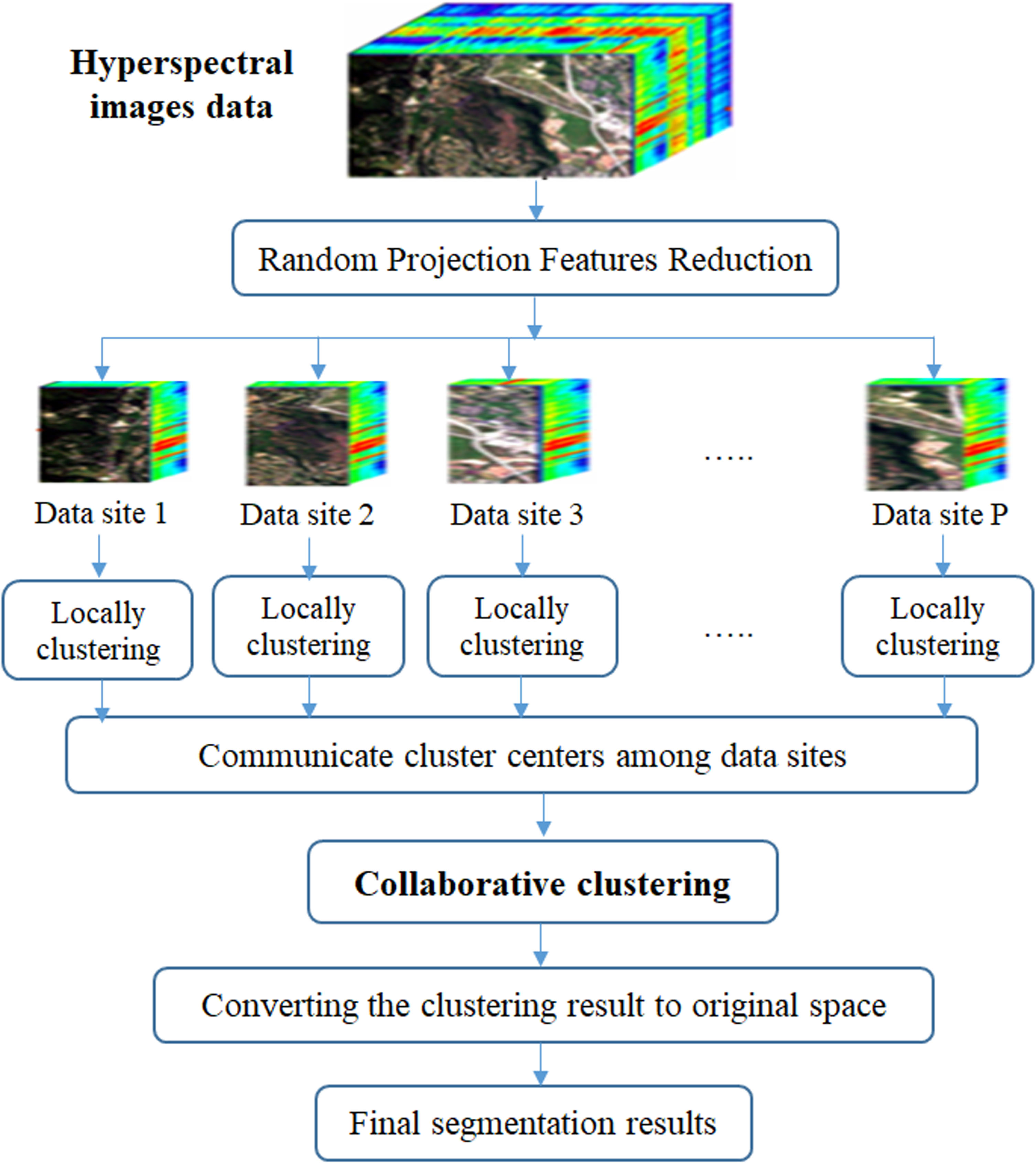
Fix x ∈ R^d, and s < k ∈ N, there exists a linear map distribution ψ_s : R^d → R^k in which, with a probability exceeding 1 - 2de^-ɛ²k/s, (0.63 - ɛ) ‖ x ‖ _1,2,s ≤ ‖ ψ_s (x) ‖ ₁ ≤ (1.63 + ɛ) ‖ x ‖ _1,2,s, where ψ_s is a random matrix with $ψ_{s} = \sqrt{2 / π} \frac{s}{k} Φ_{s}$ and Φ_s is the Hadamard (entry wise) product of two other random matrices A_s, which has d = k/s ones in a column and all other entries are filled with zero and B another random with the standard Gaussian entries that are independent and identically distributed. If s = 1, the norm, ‖x ‖ _1,2,s is reduced to the Euclidean norm. If s = d, the norm is reduced to the ℓ₁ norm denoted by ‖ . ‖ ₁. where the s represent the sparsity of x ∈ R^d and the Gaussian matrix was recovered from Φ_s.

Fig. 1

HSI segmentation diagram.

Algorithm 3 describes the steps to perform dimensionality reduction based on random projection. With input data is the HSI dataset X, the parameters epsilon ɛ, and sparsity level s. The output is the data set in a space with a smaller number of dimensions.

Algorithm 3 Random Project dimensionality Reduction

Input: Dataset X, threshold value ɛ, sparsity level s.

Begin

Step 1: Compute the value of the new dimension k.

Step 2: Find the Gaussian matrix G with (k, s).

Step 3: Find a random matrix A with 0′s and 1′s.

Step 4: Compute the Hadamard product of A, G, Φ_s.

Step 5: Calculate the random matrix $Ψ_{s} = \sqrt{2 / π} \frac{s}{k} Φ_{s}$

Step 6: Calculate the output data as a product of X and Ψ_s.

End.

Output: The data after dimensionality reduction.

Figure 3 shows how the hyperspectral remote sensing image data is processed to select important components for segmentation and minimize calculation time issues. This involves pre-processing steps such as geometry correction, image quality enhancement, and noise filtering, followed by dimensional reduction. The resulting data is then divided into P data sites. Perform local clustering using Algorithm 1 on the data sites to obtain the local centroid and membership function values of each site. These results will be used to calculate the global cluster centers for all data sites. Finally, implement a collaborative clustering algorithm on the data sites to produce the data clusters.

Algorithm 4 The FR-CFCM algorithm

Input: HSI dataset: X, the number of cluster C, the number of sub data sets P.

Begin

Phase 1: Reduce dimensions

Run Algorithm 3 to reduce dimensions of HSI data.

Phase 2: Divide data and locally clustering

1. Divide HSI data to P sub data sets.

2. Run Algorithm 1 on each sub data sets.

Phase 3: Collaborative clustering

1. Run Algorithm 2 for Collaborative clustering.

2. Give the clustered data as an output result.

3. Converting the clustered data to the original space as a final result.

End.

Output: The clustered data by partition matrix.

The proposed method is described in detail in Algorithm 4, whereby the proposed algorithm includes three phases: Reduce dimensions, divide data, and local clustering and collaborative clustering.

Computational complexity : The computational complexity of the proposed algorithm includes the computational complexity in three phases corresponding to three algorithms 1, 2, and 3. For the first phase, the computational complexity of the algorithm reduces the feature dimension. depends mainly on matrix computation with a computational complexity of O (ndkt_max). For the second phase, the computational complexity is algorithm 1, namely the FCM algorithm. The computational complexity of the second phase is O (c . n . k . P . t_max). For the third phase, the computational complexity is a collaborative clustering algorithm, which includes a computational complexity of O ((c² . n . k + c² . n . P + cnkP) * (T_max . P . t_pmax)) and the communication complexity between data sites is O (cdPT_max). Where, t_max is the maximum number of iterations on algorithms 1 and 3, T_max is the maximum number of iterations of algorithm 2, and t_pmax is the maximum number of iterations when executing local clustering on data sites where P are the number of data sites on algorithm 2, C is the number of clusters, n is the total number of pixels, d is the number of data dimensions before reduction and k is the number of data dimensions after reduce.

4 Experiments

In this section, the proposed method is evaluated by the experiments on two real HSI datasets. For collaborative clustering, after dimensionality reduction, the data sets are divided into some sub-datasets. The Xie-Beni (XB) and Partition Coefficient (PC) validity index [20] are used to compare the performance of the clustering result of the fuzzy c-means clustering algorithm (FCM) [31], the collaborative fuzzy c-means clustering algorithm (CFCM) [34], the interval type-2 fuzzy c-means clustering algorithm (IT2FCM) [46], the improved interval type-2 fuzzy c-means clustering algorithm (IT2FCM^*) [47]. The method with a greater Partition Coefficient and smaller Xie-Beni values would be the optimal solution. The PC index measures the fuzzy membership degree of final divided clusters by means of the fuzzy partition matrix, and the larger its value, the better the partition result: $PC = \frac{1}{n} \sum_{ii = 1}^{P} \sum_{r = 1}^{C} \sum_{s = 1}^{N [ii]} u_{rs} [ii]$ (11) The XB index is used to consider the membership degree and the structure of datasets which measure the overall average compactness and separateness, and the smaller its value, the better the partition result: $XB = \sum_{ii = 1}^{P} (Q [ii] / n * min_{i, j = 1, . . ., C; i \neq j} (v_{i} [ii] - v_{j} [ii]))$ (12) The resulting classification performance of the classification is evaluated by determining True Positive Rate (TPR) and False Positive Rate (FPR) defined as follows: $TPR = \frac{TP}{TP + FN}; FPR = \frac{FP}{TN + FP}$ (13) The accuracy of the classification results is calculated by the formula: $Accuracy = \frac{TP + TN}{TP + TN + FP + FN}$ (14) The indexes TP, FP, TN, and FN have the following meanings, respectively:

+ TP (True Positive): Total number of cases where the classification matches Positive.

+ TN (True Negative): Total number of cases where the classification matches Negative.

+ FP (False Positive): The total number of cases that classify the labels of the Negative label as Positive.

+ FN (False Negative): The total number of cases that classify labels belonging to the Positive label to Negative.

The algorithms are tested on the computer Intel(R) Core(TM) i5-4210U CPU @ 1.70GHz 4 processors and a hard disk of 500Gb, Windows 10 64bit operating system, 16Gb RAM, NVIDIA 2Gb graphics card. The program is written in the latest released Python language to simulate the algorithms.

4.1 Experiment 1

In this experiment 1, the HSI data is the Indian Pines dataset in the North-western Indiana area. The image data has a size of 145x145 with 200 spectral reflectance bands in the wavelength range 0.4μm - 2.4μm. The number of pixels labeled is 10, 201 pixels. The Indian Pines dataset consists of 14 land-covers including classes Alfalfa, Corn-notill, Corn-mintill, Corn, Grass-pasture, Grass-trees, Hay-windrowed, Soybean-notill, Soybean-mintill, Soybean-clean, Wheat, Woods, Building-Grass-Trees-Drives, Stone-Steel-Towers. Detailed information about the dataset and the number of pixels labeled for each layer is shown in Table 1.

Table 1
Groundtruth classes for the Indian Pines scene and their respective samples number

No. Class Sample Color

1 Alfalfa 46

2 Corn-notill 1428

3 Corn-mintill 830

4 Corn 237

5 Grass-pasture 483

6 Grass-trees 730

7 Hay-windrowed 478

8 Soybean-notill 972

9 Soybean-mintill 2455

10 Soybean-clean 593

11 Wheat 205

12 Woods 1265

13 Buildings-Grass-Trees-Drives 386

14 Stone-Steel-Towers 93

No.	Class	Sample
1	Alfalfa	46
2	Corn-notill	1428
3	Corn-mintill	830
4	Corn	237
5	Grass-pasture	483
6	Grass-trees	730
7	Hay-windrowed	478
8	Soybean-notill	972
9	Soybean-mintill	2455
10	Soybean-clean	593
11	Wheat	205
12	Woods	1265
13	Buildings-Grass-Trees-Drives	386
14	Stone-Steel-Towers	93

For collaborative clustering, after feature reduction, we split data into four sub-datasets (data site 1, data site 2, data site 3, and data site 4). When changing the value of epsilon, the number of dimensions of the data set will change, leading to a change in the accuracy of the proposed algorithm. In the experimental part, the authors tested the proposed algorithm at different values of epsilon to find the optimal value for each data set.

Based on formula 10, we can determine the relationship between the value of epsilon and the dimension after reduction in Table 2. To find the optimal epsilon value for the proposed algorithm, we set the epsilon value to increase from 0.1 to 0.9. Based on the accuracy obtained with each epsilon value, the epsilon value at 0.3 gives the highest accuracy. Note that accuracy is obtained on the entire data set. Figure 2 shows the landcover classification results from Indian Pines image data by the algorithms FCM, CFCM, IT2FCM, IT2FCM^*, and FR-CFCM. It can be seen that the FCM algorithm produces the poorest results with a lot of noise in land cover. Other algorithms produce clearer results.

Table 2

he epsilon value and their effect on the FR-CFCM algorithm for Indian Pines dataset

ϵ	0.1	0.2	0.3	0.4	0.5	0.6	0.7	0.8	0.9
Number of original dimensions	200	200	200	200	200	200	200	200	200
Number of new dimensions	130	58	26	14	9	6	5	4	3
Runtime of the FR-CFCM algorithm (s)	51.89	14.76	3.65	3.12	2.89	2.51	2.32	2.14	2.09
Accuracy of the FR-CFCM algorithm (%)	96.18	96.89	97.66	95.45	93.37	92.63	90.06	88.23	81.11

Table 2 shows the value ϵ and the number of new dimensions of the data, their influence on the execution time, and the accuracy of the proposed FR-CFCM algorithm. The value ϵ is set from small to large, including the values 0.1, 02,....., 0.8, and 0.9; At values ϵ, the number of original data dimensions is 200 bands, the new data dimensions are 130, 58, 26, 14, 9, 6, 5, 4, and 3, respectively. Performing the FR-CFCM algorithm after reducing the data dimension shows that the accuracy (Accuracy Index) reaches the maximum value of 97.66% at the value ϵ = 0.3 and the new dimension is 26. When the ϵ values are 0.1 and 0.2, the accuracy is 96.18% and 96.89% respectively. As ϵ increases, the number of data dimensions decreases and the accuracy of the FR-CFCM algorithm also decreases. The accuracy is lowest at ϵ = 0.9 with an Accuracy index of 81.11%.

In Table 2, the execution time of the FR-CFCM algorithm decreases as the value of ϵ increases. At ϵ = 0.1, the new dimension is 130, and the execution time is 51.89s; the time is reduced to 14.76s when ϵ = 0.2 and the new dimension is 58. At ϵ = 0.3, the FR-CFCM algorithm achieved the greatest accuracy and the execution time was 3.65s, about 16 times less than when ϵ = 0.1 and about 4 times less than when ϵ = 0.2; When ϵ increases from 0.3 to 0.9, the execution time of the FR-CFCM algorithm decreases but not significantly. Because there is no significant change in data dimensionality after dimensionality reduction.

Fig. 2

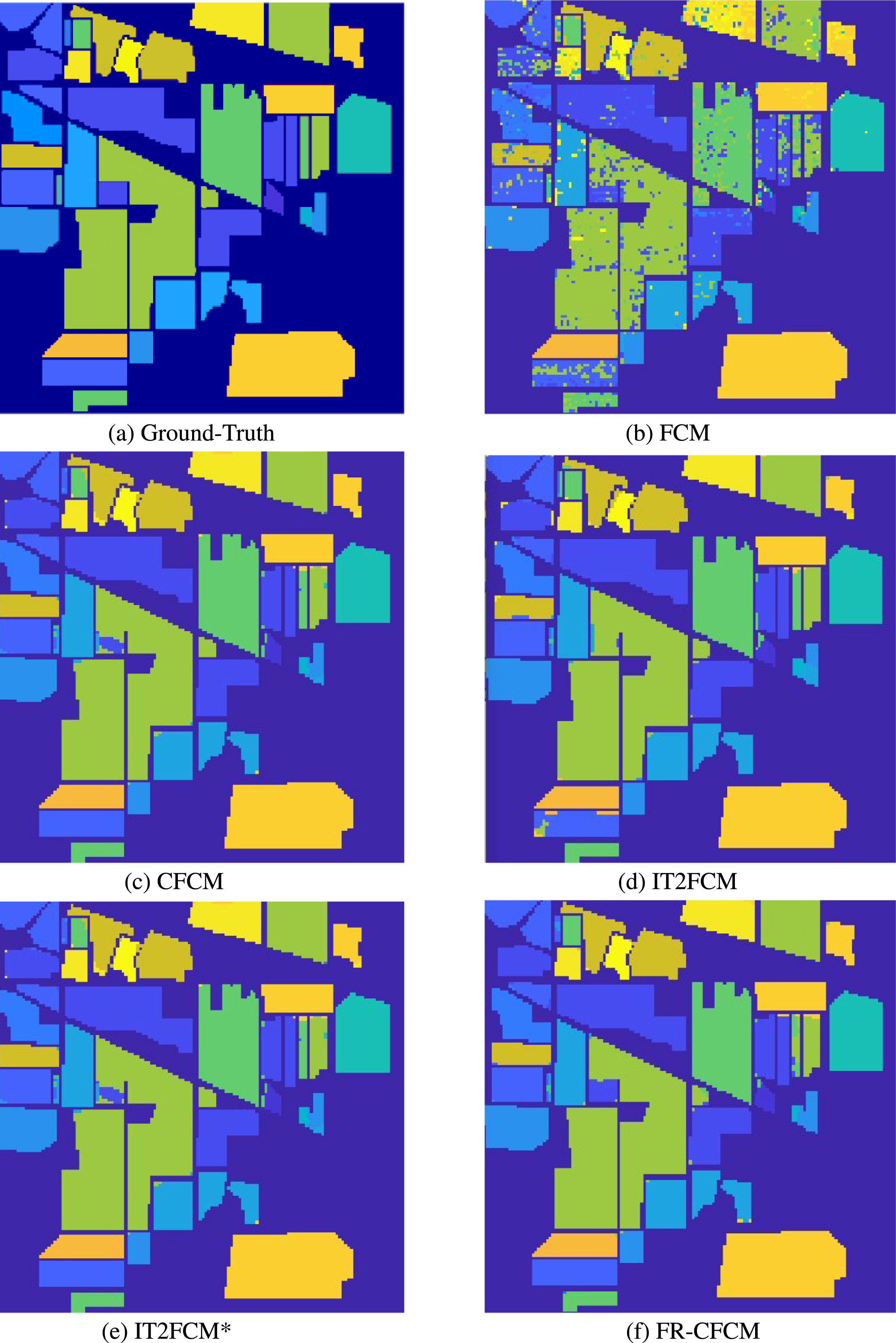
Ground-Truth and landcover classification results.

Table 3 shows the clustering quality by PC, XB, TPR, FPR, Accuracy indexes, and the execution time of the algorithms FCM, CFCM, IT2FCM, IT2FCM*, FR-CFCM. Overall, it can be seen that the FCM algorithm gives the results with the lowest accuracy. For PC and XB indexes, which are cluster quality metrics, the PC index is best at 0.456 with the IT2FCM algorithm, while the XB index achieved the best clustering result at 0.659 with the IT2FCM* algorithm. Although the FR-CFCM algorithm has PC and XB index values of 0.453 and 0.698, respectively, lower than those of IT2FCM and IT2FCM*, the difference is insignificant. This may be due to the effect of data dimensionality reduction. PC and XB indexes on FCM and CFCM algorithms give the worst results.

Table 3

Landcover classification results on Indian Pines dataset

Index	FCM	CFCM	IT2FCM	IT2FCM*	FR-CFCM
PC	0.234	0.376	0.456	0.455	0.453
XB	1.094	0.967	0.785	0.659	0.698
TPR	90.53%	95.08%	98.04%	98.35%	98.34%
FPR	5.29%	5.06%	3.28%	2.99%	1.63%
Accuracy	86.34%	94.12%	97.43%	97.45%	97.66%
Running time	7.69s	6.18s	16.87s	18.74s	3.65s

For TPR indexes, the IT2FCM* algorithm gave the highest accuracy with 98.35%, the FR-CFCM algorithm reached 98.34%, only 0.01% lower, followed by the IT2FCM algorithm with a TPR index of 98.04%. FCM and CFCM algorithms give much lower accuracy than other algorithms. While the FPR index of the FR-CFCM algorithm has the least misclassification rate with only 1.63%. Especially the Accuracy index, the FR-CFCM algorithm gives the classification results with the highest accuracy rate of 97.66%, while the IT2FCM*, IT2FCM, CFCM, and FCM algorithms are 97.45%, 97.43%, 94.12%, and 86.34%, respectively.

Regarding the execution time of the algorithms, it can be seen that FR-CFCM has the fastest execution time with 3.65s compared to 6.18s for CFM, 7.69s for FCM, 16.87s for IT2FCM and 18.74s for IT2FCM*.

In general, with the Accuracy index FR-CFCM algorithm gives the best results, while the PC and XB indices of IT2FCM, IT2FCM*, and FR-CFCM algorithms are higher than those of FCM and CFCM algorithms. This can be explained that the data dimensionality reduction method in the FR-CFCM algorithm can keep quite well the basic characteristics of the data, helping the FR-CFCM algorithm achieve much higher accuracy than CFCM. While the data representation based on the interval type 2 fuzzy set in the IT2FCM and IT2FCM* algorithms can help improve the accuracy. However, the execution time of the IT2FCM and IT2FCM* algorithms is about 6 times slower than that of the FR-CFCM algorithm, and the execution time of the FCM and CFCM algorithms is about 2 times slower than that of FR-CFCM.

4.2 Experiment 2

Fig. 3

Ground-Truth and landcover classification results.

The data used in experiment 2 is the Pavia University dataset. These are the scenes acquired by the ROSIS sensor during a flight campaign over Pavia, northern Italy. This dataset has 103 spectral bands with an image size of 610x610 and a spatial resolution of 1.3 meters. The data is classified into nine different classes including Asphalt, Meadows, Gravel, Trees, Painted metal sheets, Bare Soil, Bitumen, Self-Blocking Bricks, and Shadows. The number of sample data is 42, 776 pixels. Detailed information on the number of samples for each class is shown in Table 5.

For collaborative clustering, after feature reduction, we also split data into four sub-datasets (data site 1, data site 2, data site 3, and data site 4). Based on formula 10, we determine the relationship between the value of epsilon and the dimension after reduction in Table 4. For the Pavia University dataset, the accuracy of the proposed algorithm reaches the optimal value at epsilon equal to 0.4. Note that accuracy is obtained on the entire data set.

Table 4

The epsilon value and their effect on the FR-CFCM algorithm for Pavia University dataset

ϵ	0.1	0.2	0.3	0.4	0.5	0.6	0.7	0.8	0.9
Number of original dimensions	103	103	103	103	103	103	103	103	103
Number of new dimensions	101	50	22	13	8	6	4	3	2
Runtime of the FR-CFCM algorithm (s)	286.33	110.38	42.18	27.47	20.85	13.44	9.51	8.07	7.74
Accuracy of the FR-CFCM algorithm (%)	95.99	96.39	96.21	96.41	94.32	91.09	87.26	83.63	79.28

From the original data’s dimensionality of 103, after dimensionality reduction, the dimensionality is reduced to 101 (at ϵ = 0.1), 50 (at ϵ = 0.2), and so on. Table 4 shows that when the number of dimensions is greater than 8, the accuracy of the FR-CFCM algorithm is quite high, about 96%. Meanwhile, when the number of dimensions is less than 8, the accuracy drops sharply from 94.32% to 79.28%. The FR-CFCM algorithm achieves the largest Accuracy index of 96.41% at ϵ = 0.4 and the new dimension is 13.

Table 4 also shows that the execution time of the algorithm is proportional to the dimensionality of the data. When the data dimension is 101, the execution time of the FR-CFCM algorithm is 286.33s and decreases to 110.38s when the data dimension is 50. When the number of dimensions is 2, the execution time of the FR-CFCM algorithm is reduced to as low as 7.74s.

Table 5 shows the land cover of different colors. The classification results are shown in Figure 3 with image data and results from 5 different algorithms including FCM, CFCM, IT2FCM, IT2FCM*, and FR-CFCM.

Table 5

Groundtruth classes for the Pavia University scene and their respective samples number

No.	Class	Sample	Color
1	Asphalt	6631
2	Meadows	18649
3	Gravel	2099
4	Trees	3064
5	Painted metal sheets	1345
6	Bare Soil	5029
7	Bitumen	1330
8	Self-Blocking Bricks	3682
9	Shadows	947

In Table 6, the FR-CFCM algorithm gives the best classification results in most indicators, followed by the IT2FCM and IT2FCM* algorithms, while the FCM and CFCM algorithms give the worst results. Specifically, the FR-CFCM algorithm gives the best classification results in TPR, FPR, Accuracy, and Running time indexes. With the PC index, the FR-CFCM algorithm reached 0.653 compared to 0.674 of the IT2FCM* algorithm and 0.672 of the IT2FCM algorithm. While the two algorithms FCM and CFCM have PC index values of 0.481 and 0.583, respectively. Similar to the XB index, the FR-CFCM algorithm reached 0.677 higher than the IT2FCM and IT2FCM* algorithms, but the difference was not significant. The FCM and CFCM algorithms gave the worst classification results with the XB index of 0.895 and 0.799, respectively.

Table 6

Landcover classification results on Pavia University dataset

Index	FCM	CFCM	IT2FCM	IT2FCM*	FR-CFCM
PC	0.481	0.583	0.672	0.674	0.653
XB	0.895	0.799	0.647	0.628	0.677
TPR	88.56%	92.95%	95.03%	96.17%	96.89%
FPR	4.27%	3.61%	3.52%	2.26%	1.88%
Accuracy	86.62%	93.78%	94.11%	96.29%	96.41%
Running time	41.04s	35.37s	183.82s	210.81s	27.47s

For TPR, FPR, and Accuracy indexes, the FR-CFCM algorithm gives the best results with the highest correct classification rate of 96.89% and the smallest false classification rate of 1.88%. Overall accuracy also reached the highest at 96.41% with the FR-CFCM algorithm. Meanwhile, these values are lowest with the FCM algorithm, followed by CFM, IT2FCM, and IT2FCM* algorithms.

Regarding the execution time of the algorithms, the FR-CFCM algorithm has the fastest execution time with 27.47s, while the IT2FCM* algorithm has the slowest with 219.81s. The algorithms IT2FCM and IT2FCM* based on interval type 2 fuzzy set give higher accuracy than algorithms FCM and CFCM, but the computation time is quite slow.

From the results in Tables 2 and 4, it can be concluded that the computation time is proportional to the number of dimensions of the data because the larger the number of dimensions, the greater the computational complexity. In addition, the use of multiple data dimensions does not guarantee the highest accuracy, this is because HSI data has many spectral channels, spectral channels are received by different bands of electromagnetic waves and are therefore useful for different problems. The dimensional transformation not only reduces the computation time but also preserves the important characteristics of the data, thereby not reducing the accuracy of the classification results.

With both Tables 3 and 6, it can be seen that the FR-CFCM algorithm has the highest classification accuracy among the five experimental algorithms, and the computation time is also the fastest. Meanwhile, PC and XB cluster quality index values are nearly equivalent to IT2FCM, IT2FCM* and much better than FCM, and CFCM.

The above experiments show that the epsilon value will be adjusted for each dataset. Due to the complexities of hyperspectral image data, it is difficult to give a specific optimal epsilon value for all data sets. In this study, we recommend that when using the algorithm, experiment on different epsilon values to find the best value for each data set.

5 Conclusion

This study focuses on the challenges of HSI segmentation, which includes the high number of dimensions and data instances. The paper proposes a new method to tackle these issues by utilizing collaborative clustering and reducing data dimensions based on the JL lemma. We believe this approach will be effective in HSI segmentation. The experiments subsequently indicate that the proposed method produces better results with regard to validity indexes and running time. The experimental results on 02 datasets of hyperspectral remote sensing images show that the proposed algorithm FR-CFCM gives better results than the algorithms FCM, CFCM, IT2FCM, and IT2FCM^*.

In future research, we aim to propose an algorithm to automatically find the optimal epsilon value on each data set. Moreover, we will develop algorithms based on parallel computing models to improve algorithm performance when working with large data sets.

Footnotes

Declarations

The authors declare that they have no known competing financial interests or personal relationships that could have appeared to influence the work reported in this paper.

Author Contribution Statement

The authors confirm their contribution to the paper as follows: study conception and design: Trong Hop Dang, Viet Duc Do, Dinh Sinh Mai; data collection: Viet Duc Do, Le Hung Trinh; analysis and interpretation of results: Viet Duc Do, Dinh Sinh Mai, Trong Hop Dang, Long Thanh Ngo, Le Hung Trinh; draft manuscript preparation: Viet Duc Do, Dinh Sinh Mai, Le Hung Trinh. All authors reviewed the results and approved the final version of the manuscript.

References

Yuan

, Lin

and Wang

, Dual-clustering-based hyperspectral band selection by contextual analysis, IEEE Transactions on Geoscience and Remote Sensing 54 (2016).

Jia

, Tang

, Zhu

and Li

, A novel ranking-based clustering approach for hyperspectral band selection, IEEE Transactions on Geoscience and Remote Sensing 54 (2016).

Feng

, Jiao

, Sun

, Liu

and Zhang

, Multiple kernel learning based on discriminative kernel clustering for hyperspectral band selection, IEEE Transactions on Geoscience and Remote Sensing 54 (2016).

, Liu

, Cai

and Cai

, Band selection of hyperspectral images using multiobjective optimization-based sparse self-representation, IEEE Geoscience and Remote Sensing Letters 16 (2019).

Duan

, Huang

, Tang

, Li

and Pu

, Semi-supervised manifold joint hypergraphs for dimensionality reduction of hyperspectral image, in IEEE Geoscience and Remote Sensing Letters 18(10) (2021), 1811–1815.

Zeng

, Cai

, Liu

, Hu

and Ku

, Unsupervised hyperspectral image band selection based on deep subspace clustering, IEEE Geoscience and Remote Sensing Letters 16 (2019).

Imani

and Ghassemian

, Band clustering-based feature extraction for classification of hyperspectral images using limited training samples, IEEE Geoscience and Remote Sensing Letters 11 (2014).

Archibald

and Fann

, Feature selection and classification of hyperspectral images with support vector machines, IEEE Transactions on Geoscience and Remote Sensing 4 (2007).

Wang

, Liang

, Xu

, Song

, Wang

and Huang

, Dimensionality reduction method for hyperspectral image analysis based on rough set theory, European Journal of Remote Sensing 53(1) (2020), 192–200.

10.

Paul

and Chaki

, Dimensionality reduction of hyperspectral images using pooling, Pattern Recognit Image Anal 29 (2019), 72–78.

11.

Aréchiga

, Barocio

, Ayon

J.J.

and Garcia-Baleon

H.A.

, Comparison of Dimensionality Reduction Techniques for Clustering and Visualization of Load Profiles, Jalisco, in IEEE PES Transmission and Distribution Conference and Exposition, 2016.

12.

Bishnu

S.P.

and Bhattacharjee

, A Dimension Reduction Technique for K-Means Clustering Algorithm, Dhanbad, India, in International Conference on Recent Advances in Information Technology, 2012.

13.

Lupu

, Necoara

, Garrett

J.L.

and Johansen

T.A.

, Stochastic higher-order independent component analysis for hyperspectral dimensionality reduction, in IEEE Transactions on Computational Imaging 8 (2022), 1184–1194.

14.

Feng

, Liu

, Yang

, Zhang

and Jiao

, Hierarchical feature fusion and selection for hyperspectral image classification, in IEEE Geoscience and Remote Sensing Letters 20 (2023), 1–5.

15.

Jiang

, Xiong

, Yan

, Zhang

, Liu

and Cai

, Unsupervised dimensionality reduction for hyperspectral imagery via laplacian regularized collaborative representation projection, in IEEE Geoscience and Remote Sensing Letters 19 (2022), 1–5.

16.

Tarabalka

, Fauvel

, Chanussot

and Benediktsson

J.A.

, SVM- and MRF-based method for accurate classification of hyperspectral images, IEEE Geoscience and Remote Sensing Letters 7 (2010).

17.

Melgani

and Bruzzone

, Classification of hyperspectral remote sensing images with support vector machines, IEEE Transactions on Geoscience and Remote Sensing (2004).

18.

Zhang

, Zhai

, Zhang

and Li

, Spectral–spatial sparse subspace clustering for hyperspectral remote sensing images, IEEE Transactions on Geoscience and Remote Sensing (2016).

19.

Camps-Valls

and Bruzzone

, Kernel-based methods for hyperspectral image classification, IEEE Transactions on Geoscience and Remote Sensing 43 (2005).

20.

Zhou

, Kwan

, Ayhan

and Eismann

M.T.

, A novel cluster kernel RX algorithm for anomaly and change detection using hyperspectral images, IEEE Transactions on Geoscience and Remote Sensing (2017).

21.

Bernabe

, Marpu

P.R.

, Plaza

, Mura

M.D.

and Benediktsson

J.A.

, Spectral– spatial classification of multispectral images using kernel feature space representation, IEEE Geoscience and Remote Sensing Letters 11 (2014).

22.

Senthilnath

, Kulkarni

, Benediktsson

J.A.

and Yang

X.S.

, A novel approach for multispectral satellite image classification based on the bat algorithm, IEEE Geoscience and Remote Sensing Letters (2016).

23.

Ghamisi

, Ali

A.-R.

, Couceiro

M.S.

and Benediktsson

J.A.

, A novel evolutionary swarm fuzzy clustering approach for hyperspectral imagery, IEEE Journal of Selected Topics in Applied Earth Observations and Remote Sensing 8 (2015).

24.

Yang

, Qiao

, Yang

, Jin

and Jiao

, Hyperspectral image classification based on relaxed clustering assumption and spatial laplace regularizer, IEEE Geoscience and Remote Sensing Letters 11 (2014).

25.

Kong

, Cheng

, Chen

C.L.P.

and Wang

, Hyperspectral image clustering based on unsupervised broad learning, IEEE Geoscience and Remote Sensing Letters 16 (2019).

26.

, Bioucas-Dias

J.M.

and Plaza

, Spectral– spatial classification of hyperspectral data using loopy belief propagation and active learning, IEEE Transactions on Geoscience and Remote Sensing (2013).

27.

Bernard

, Tarabalka

, Angulo

, Chanussot

and Benediktsson

J.A.

, Spectral–spatial classification of hyperspectral data based on a stochastic minimum spanning forest approach, IEEE Transactions on Image Processing (2012).

28.

, Zhang

, Kang

, Wang

and Benediktsson

J.A.

, Spatial density peak clustering for hyperspectral image classification with noisy labels, IEEE Transactions on Geoscience and Remote Sensing (2019).

29.

Kanungo

, Mount

D.M.

, Netanyahu

N.S.

, Piatko

C.D.

, Silverman

and Wu

A.Y.

, An efficient k-means clustering algorithm: Analysis and implementation, IEEE Trans On Pattern Analysis and Machine Intelligence 24(7) (2002), 881–893.

30.

Zalik

K.R.

, An efficient k-means clustering algorithm, Pattern Recognition Letters 29 (2008), 1385–1391.

31.

Bezdek

J.C.

, Ehrlich

and Full

, FCM: The fuzzy c-means clustering algorithm, Computers and Geosciences 10(2-3) (1984), 191–203.

32.

Zhu

, Chung

F.L.

and Wang

, Generalized fuzzy C-means clustering algorithm with improved fuzzy partitions, IEEE Trans On Systems, Man, and Cybernetics, Part B: Cybernetics 39(3) (2009), 578–591.

33.

Maji

and Pal

S.K.

, Rough set based generalized fuzzy CMeans algorithm and quantitative indices, IEEE Trans On Systems, Man, and Cybernetics, Part B: Cybernetics (2007), 1529–1540.

34.

Pedrycz

, Collaborative fuzzy clustering, Pattern Recognition Letters 23 (2002), 1675–1686.

35.

Pedrycz

, Collaborative clustering with the use of Fuzzy C-Means and its quantification, Fuzzy Sets and Systems (2008), 2399–2427.

36.

Mai

D.S.

and Dang

T.H.

, An improvement of collaborative fuzzy clustering based on active semi-supervised learning, 2022 IEEE International Conference on Fuzzy Systems (FUZZ-IEEE), Padua, Italy 2022, pp. 1–6 .

37.

Pedrycz

, Collaborative, and knowledge-based fuzzy clustering, International Journal of Innovative Computing, Information and Control 3 (2007), 1–12.

38.

Coletta

L.F.S.

, Vendramin

, Hruschka

E.R.

, Campello

R.J.G.B.

and Pedrycz

, Collaborative fuzzy clustering algorithms: Some refinements and design guidelines, IEEE Transaction on Fuzzy Systems (2012), 444–462.

39.

Zhou

, Chen

C.L.P.

, Chen

and Li

H.X.

, Collaborative fuzzy clustering algorithm in distributed network environments, IEEE Trans on Fuzzy Systems (2014), 1–14.

40.

Jiang

, Chung

F.L.

, Wang

, Deng

, Wang

and Qian

, Collaborative fuzzy clustering from multiple weighted views, IEEE Trans on Cybernetics (2014), 1–13.

41.

Prasad

, Li

D.L.

, Liu

Y.T.

, Siana

, Lin

C.T.

and Saxena

, A Preprocessed Induced Partition Matrix Based Collaborative Fuzzy Clustering For Data Analysis, IEEE International Conference on Fuzzy Systems (2014), pp. 1553–1558.

42.

John

A.L.

and Michael

, Two Key properties of Dimensionality reduction methods, in Computational Intelligence and Data Mining (CIDM), Orlando, FL, USA, 2014.

43.

Johnson

and Lindenstraus

, Extensions of Lipshotz mapping into Hilbert space, in Contemporary Mathematics, Texas, 1984.

44.

Dimitris

, Database-friendly random projections: Johnson-Lindenstrauss with binary coins, Journal of Computer and System Sciences 63 (2003), 271–678.

45.

Felix

and Rachael

, A unified framework for dimensionality reduction in L1, Results In Mathematics 70(1-2) (2016), 209–231.

46.

Hwang

and Rhee

F.C.H.

, Uncertain fuzzy clustering: Interval Type-2 fuzzy approach to C-Means, IEEE Trans Fuzzy Syst 15(1) (2007), 107–120.

47.

Guo

and Huo

, An enhanced IT2FCM* algorithm integrating spectral indices and spatial information for multi-spectral remote sensing image clustering, Remote Sensing 9(9) (2017), 960.