Application of fuzzy support vector regression machine in power load prediction

Abstract

Power system load forecasting is a method that uses historical load data to predict electricity load data for a future time period. Aiming at the problems of general prediction accuracy and slow prediction speed in using typical machine learning methods, an improved fuzzy support vector regression machine method is proposed for power load forecasting. In this method, the boundary vector extraction technique is employed in the design of the membership function for fuzzy support vectors to differentiate the importance of different samples in the regression process. This method utilizes a membership function based on boundary vectors to assign differential weights to different sample points that used to differentiate the importance of different types of samples in the regression analysis process in order to improve the accuracy of electricity load prediction. The key parameters of the fuzzy support vector regression model are optimized, further enhancing the precision of the forecasting results. Simulation experiments are conducted using real power load data sets, and the experimental results demonstrate the effectiveness of the proposed method in terms of accuracy and speed in predicting power load data compared to other prediction models. This method can be widely applied in real power production and scheduling processes.

Keywords

Machine learning fuzzy support vector regressive machine power load prediction membership function boundary vector

1 Introduction

Power load forecasting refers to the use of historical load data to predict the load values for a future time period. It has become an important component of achieving modernization in power system management. It finds wide-ranging applications in formulating generator unit combinations, inter-regional power transmission schemes, and load dispatching plans within the power system. Improving the accuracy of load forecasting effectively contributes to the economic and secure operation of the power system and serves as a vital basis for rational power system scheduling, planning, electricity distribution, and development [1].

With the emergence and rapid development of machine learning and artificial intelligence models, related theories and methods have been widely used to solve complex problems in engineering applications and scientific fields. Khalid Elbaz et al. proposed a new model to estimate the disc cutter life that used in shield tunnel by integrating a group method of data handling (GMDH)-type neural network (NN) with a genetic algorithm (GA), and the research results are helpful to the rational planning of shield tunnel [2]. Wafaa Shaban used the salp swarm algorithm (SSA) with the differential evolution technique (DE) via a multi-objective fitness function to predict the compressive strength of the volcanic ash material (RAC). It provides an effective method for predicting the physical properties of RAC [3]. Tao Yan et al. utilized the Bayesian optimization machine-learning algorithm to forecast the long-term trend of water quality changes. The research findings offer valuable technical support for emergency water pollution control [4]. Yu-Lin Chen et al. used the estuarine trophic state assessment method (ASSETS) and Monte Carlo simulation method (MCS) to predict the risk level of red tide in the coastal area, which can provide an effective risk assessment scheme for red tide management [5].

Machine learning algorithms have strong data mining and fitting capabilities, which can better deal with strong randomness problems and provide new ideas for power load forecasting. With the emergence of the Artificial Neural Network (ANN) model, researchers have applied its adaptive function to a large number of non-structural and imprecise rules for power load prediction. However, as the research has progressed, the final convergence of artificial neural networks heavily depends on the initial set point, resulting in slow convergence, local extreme value problems, and weak autonomous learning ability due to algorithmic defects. These limitations prevent breakthroughs in existing research results, and only local improvements or combinations with other methods have achieved better convergence in load prediction [6]. The Artificial Bee Colony (ABC) algorithm is also commonly applied in electricity load forecasting. The ABC method has a relatively large number of load forecasting parameters, but its setting is simple. It excels at processing noisy data and exhibits strong robustness. However, its implementation method is complex. Because of the characteristics of random search data set, the convergence speed of ABC is slow and it is easy to generate local optimal solution, which leads to low prediction accuracy.

Support vector machine (SVM) [7] is a prediction method based on statistical theory. Because of its good nonlinear data processing ability and be used to deal with power load forecasting problems. SVM is essentially a classical quadratic programming problem. Compared with ANN and ABC, SVM has faster convergence speed and effectively avoids local optimal solutions, and it can use many mature algorithms in optimization theory. However, it is sensitive to noise data, which makes its prediction accuracy not significantly improved compared with ANN and ABC.

Compared with Support Vector Machines (SVM), Support Vector Regression Machine (SVRM) uses more appropriate loss functions and kernel functions. It combines membership functions to reflect the importance of data samples to the regression plane, determining the weights of data samples in the load forecasting process. This helps to mitigate the impact of noisy data on the load forecasting process and improve its predictive performance. Because of these advantages, SVRM is widely used in power load forecasting.

Recently, scholars have done a lot of work on power load forecasting using SVRM method. In 2021, Fan Guo-Feng et al. proposed a hybrid short-term load forecasting model based on support vector regression (SVR) and random forest (RF). The experimental results show that this model has high prediction accuracy for power load forecasting [8]. In 2022, Wang Rui et al. proposed a fuzzy support vector machine based on geometric algebra, named Clifford fuzzy support vector machine for regression (CFSVR). The weights of different input points are determined by fuzzy membership degree with respect to the optimal regression hyperplane. The experimental results show that CFSVR can improve the accuracy of power load forecasting and realize multi-step forecasting [9]. Zhang Weiguo et al. proposed a hybrid model that combines logarithmic spiral, firefly algorithm and support vector regression (LS-FA-SVR). Compared with the benchmark model, the LS-FA-SVR hybrid model has higher prediction accuracy [10]. Luo Jian et al. proposed a robust support vector regression (RSVR) model to realize the power load forecasting model in 2023. By introducing a weight function to calculate the relative weight of each observed value in the load history, a weighted quadric surface SVR model is constructed. This method improves the prediction accuracy of the RSVR model [11].

SVRM has good predictive ability. It can approach nonlinear functions with arbitrary precision, and has the advantages of global minimum points, fast Rate of convergence. SVRM has good prediction ability. It can approximate nonlinear functions with arbitrary precision, and has the advantages of global minimum point and fast convergence speed [12]. It also has the problem of rapid decline in training speed and accuracy due to the large increase in the number of training samples. The main reason is that the classical membership function determines the membership degree by the distance between the sample data and the regression plane, and the membership degree of the data far away is small. Some noise data are close to the regression plane, but far away from most data samples. This kind of noise data is also called outliers have a great influence on training accuracy and speed.

In order to solve the above problems, the authors propose a fuzzy SVR algorithm based on boundary vector extraction (BVE-FSVR). BVE-FSVR algorithm is to find the minimum hypersphere that can contain the effective sample points in the feature space to replace the regression plane which used by the traditional membership function. BVE-FSVRM algorithm is to use the distance between the sample point and the center of the hypersphere as the membership value of the sample data instead of using the distance between the sample point and the regression plane. BVE-FSVRM algorithm can more effectively distinguish the importance of different samples in the training process, greatly reduce the influence of noise data to improve the training accuracy, and reduce the number of training samples to improve the training speed [13].

2 Support vector repressor machine and the training algorithm

The classical SVM algorithm is an important machine learning method proposed by Vapnik, SVM aims to minimize the upper limit of the generalization error by maximizing the margin between separating the hyperplane and the data, providing a basis for the structural risk minimization principle [14]. Support vector regression for SVR is an important branch of application in SVM. The difference between SVR regression and SVM classification is that the SVR finally has only one class, and the optimal superplane it seeks is not to “maximize” the distance between two or more class samples as the SVM does, but to “minimize” all sample points from the superplane [15].

2.1 Loss function

SVR can be used in functional regression analysis, and the accuracy of the estimation process is estimated by constructing the appropriate loss function. The loss function is used to evaluate the degree to which the predicted value and the true value differ, and the selection of the loss function usually determines the model performance [16]. The loss function is divided into the empirical risk loss function and the structural risk loss function. The empirical risk loss function refers to the difference between the predicted results and the actual results, and the structural risk loss function refers to the empirical risk loss function plus a regular term. Several common loss functions are used as follows.

(1) 0-1 loss function: 0-1 loss function is the earliest loss function proposed by Cortes and Vapnik et al. [7]. It is discontinuous at t = 0, and is a non-convex continuous bounded function. This discontinuity makes it unsuitable for traditional optimization theories and methods. $L_{0 / 1} (t) = {\frac{1, t > 0}{0, t ⩽ 0}$ (1)

(2) Hinge loss function: Hinge loss function is also proposed by Cortes and Vapnik et al. [7]. The hinge loss function is the best convex approximation of the 0-1 loss function. If t≤0, the loss value is 0, indicating that it has no loss to the correctly divided samples and has good sparsity. If t > 0, the loss value is t, indicating that it has a large contribution weight to the SVM objective function and affects the solution of the optimal hyperplane. $L_{HL} (t) = {\frac{t, t > 0}{0, t ⩽ 0}$ (2)

(3) Logarithmic loss function: Wahba introduced the logarithmic loss function into SVM in 1998 [17]. Different from the hinge loss function, it gives the logarithmic loss to all samples, and this characteristic makes it not sparse and sensitive to outliers. $L_{LL} (t) = \log (1 + \exp (t - 1)), t \in R$ (3)

(4) Pinball loss function: In 2013, Jumutc et al. proposed the pinball loss function [18]. If τ= 0, it degenerates into the hinge loss function. The loss value is – τ. when t≤0, so it does not have sparsity and sensitive to outliers. $L_{PL} (t) = {\begin{matrix} t, t > 0 \\ - τ t, t ⩽ 0 \end{matrix}$ (4)

(5) ɛ-insensitive pinball loss function: In order to overcome the shortcomings of the pinball loss function that is not sparse, Xiaolin Huang et al. proposed the ɛ-insensitive pinball loss function (ɛ-i PLF) in 2014 [19]. Different from the pinball loss function, the ɛ-insensitive pinball loss function sets different values through different ranges of parameter t to ensure sparsity and reduce its outlier sensitivity. The ɛ-i PLF is used in the method proposed by the author. $L_{i - PL} (t) = {\begin{matrix} t - ɛ, t > ɛ \\ 0, t \in [- \frac{ɛ}{τ}, ɛ] \\ - τ (t + \frac{ɛ}{τ}), t < - \frac{ɛ}{τ} \end{matrix}$ (5)

2.2 Linear regression

Considering the training sample data set (x₁, y₁) , (x₂, y₂) , . . . , (x_n, y_n), if the input data sample is linearly separable, then the hyperplane can be represented as w × x + b = 0, and a function of the sample point x_i can be obtained: $\begin{matrix} f (x) = sign (w \cdot x_{i} + b) = {\begin{matrix} 1, y_{i} = 1 \\ - 1, y_{i} = - 1 \end{matrix}} \\ s . t . i = 1, 2 . . . ., l \end{matrix}$ (6)

The ɛ-i PLF is introduced, and rewritten it into an equation form suitable for linear regression, as shown in Equation (7). $c (x, y, f (x)) = max {0, | y - f (x) | - ɛ}$ (7)

In the above equation, ɛ is a positive value taken in advance. The ɛ-i PLF shows that when the difference between the observed value y and the predicted value of the point f (x) does not exceed the previously determined value ɛ, then the predicted value at the point f (x) is considered as no loss.

Finding parameter pairs (ω, b) makes a small possible deviation between the function f (x) and the actual acquisition target y_i, while also making it as smooth as possible. To maximize the remainder in the linearly separable case, and as shown in Equation (8). ${\begin{matrix} min \frac{1}{2} {‖ w ‖}^{2} \\ y_{i} (w^{T} x_{i} + b) ⩾ 1 i = 1, 2, . . . . . . \end{matrix}$ (8)

w is the weight vector, and b is the amount of deviation. For linear inseparability, all constraints are impossible to meet in Equation (8), then the violation of constraints measured using relaxation variables ɛ_i, i ∈ (1, 2, . . . . . . , l), Equation (8) can be converted into Equation (9). ${\begin{matrix} min \frac{1}{2} {‖ w ‖}^{2} + C \sum \begin{matrix} l \\ i = 1 \end{matrix} ξ_{i} \\ y_{i} (w^{T} x_{i} + b) ⩾ 1 - ξ_{i}, ξ_{i} ⩾ 0 \forall i = 1, 2, . . ., l \end{matrix}$ (9)

In the Equation (9), C is a constant, the larger the value of C, the less the training misclassification of SVM, the smaller the marginal value; on the contrary, the decrease of C will cause the SVM to ignore more training points, resulting in the swing amplitude of the convergence result is more [20].

To facilitate the calculations, Lagrangian is introduced and simultaneously simplified by the corresponding saddle point conditions: $\begin{matrix} min_{α} \frac{1}{2} \sum_{i = 1}^{l} \sum_{j = 1}^{l} (a_{i}^{*} - a_{i}) (a_{j}^{*} - a_{j}) (x_{i}, x_{j}) \\ + ɛ \sum_{i = 1}^{l} (a_{i}^{*} + a_{i}) - \sum_{i = 1}^{l} y_{i} (a_{i}^{*} - a_{i}) \\ s . t . \sum_{i = 1}^{l} (α_{i} - α_{i}^{*}) = 0, α_{i}, a_{i}^{*} \in [0, C] \end{matrix}$ (10)

Where $a = (a_{1}, . . ., a_{l})^{T}, a^{*} = (a_{1}^{*}, . . ., a_{l}^{*})^{T}, a_{i},$ $a_{i}^{*}$ for the Lagrange multiplier corresponding to the sample, the optimal solution is $a^{(*)} = (a_{1}, a_{1}^{*}, . . ., a_{i}, a_{i}^{*})^{T}$ , only a small fraction of the solution is non-zero, and the corresponding sample is support vector [21]. The values of w and b can be calculated as shown in Equation (11). $\begin{matrix} w = \sum_{i = 1}^{l} (a_{i}^{*} - a_{i}) x_{i} \\ b = y_{j} - \sum_{i = 1}^{l} (a_{i}^{*} - a_{i}) (x_{i}, x_{j}) - ɛ \end{matrix}$ (11)

The regression function of the available SVM is: $f (x) = w^{T} x + b = \sum_{i = 1}^{m} (a_{i}^{*} - a_{i}) (x_{i}, x) + b$ (12)

2.3 Non-linear regression

Nonlinear regression usually uses a nonlinear transformation φ to transform the input space into a high-dimensional feature space to solve the optimal regression function. The calculation of φ and the regression function involved in the feature space is expressed in the form of the inner product of φ, and the kernel function K (x, x_i) = (φ (x) , φ (x_i)) is introduced to replace the inner product operation of φ, as shown in Equations (13) to (15): $\begin{matrix} min \frac{1}{2} \sum_{i = 1}^{l} \sum_{j = 1}^{l} (a_{i}^{*} - a_{i}) (a_{j}^{*} - a_{j}) K (x_{i}, x_{j}) \\ + ɛ \sum_{i = 1}^{l} (a_{i}^{*} + a_{i}) - \sum_{i = 1}^{l} y_{i} (a_{i}^{*} - a_{i}) \\ s . t . \sum_{i = 1}^{l} (a_{i} - a_{i}^{*}) = 0, a_{i}, a_{i}^{*} \in [0, C] \end{matrix}$ (13) $b = y_{j} - \sum_{i = 1}^{l} (a_{i}^{*} - a_{i}) K (x_{i}, x_{j}) - ɛ$ (14) $f (x) = \sum_{i = 1}^{l} (a_{i}^{*} - a_{i}) K (x_{i}, x) + b$ (15)

The kernel function K (x, x_i) is an important part of SVR, which allows SVR to efficiently handle high-dimensional problems with finite samples. The reference kernel function can transform the non-linear no separable data sample into the linear separable data sample in high-dimensional space, which effectively solves the problem of large mathematical operations in high-dimensional space.

Set the attribute quantity of the kernel function σ, the kernel function can be defined using Equation (16) $k_{ij} = \exp (- \frac{{‖ x_{i} - x_{j} ‖}^{2}}{σ}), σ \in (1, 2, 3, . . ., l)$ (16)

3 Design of the fuzzy support vector regression machine algorithm

3.1 Fuzzy support vector regressive machine algorithm

The concept of Fuzzy SVM (FSVM) was proposed by Lin C F in 2002 [22], the FSVM makes different input sample points contribute differently to the decision plane, and the proposed method improves the SVM ability against noise and is especially suitable for not fully revealing the input sample features. Despite its good learning performance and generalization ability, the SVM is sensitive to noise, causing model overfitting, and for specific sequences, each sample makes different contributions to the hyperplane. Therefore, the fuzzy support vector regression (FSVR) machine method is introduced to effectively distinguish the noise and the effective samples by constructing the FSVR, in order to improve the accuracy of the model and minimize the error.

Ideally, the selection of parameters based on minimizing the generalization error of the learning machine, while in practice, the generalization error of the learning machine is impossible when the distribution function is unknown, so the generalization error is estimated. The estimation of the generalization error is the basis of model selection as well as parameter optimization [10].

For the given training data (x₁, y₁) , (x₂, y₂) , ·· · , (x_i, y_i) ∈ Rⁿ × R, the training sample x_i can be mapped to the Hilbert feature space through the nonlinear mapping φ, and the unknown function is estimated in the feature space with the linear function f (x) = (w × φ (x)) + b, then the Equation (17) can be used to solve the optimization problem: $\begin{matrix} min \frac{1}{2} w^{T} w + C \sum_{i = 1}^{l} (s_{i} ξ_{i}) \\ s . t . y_{i} (w^{T} * φ (x_{i})) + b ⩾ 1 \\ ξ_{i}, i = 1, 2, . . ., l \end{matrix}$ (17)

The corresponding decision function can solve using the following functions. $\begin{matrix} f (x) = \sum_{i = 1}^{l} (a_{i} y_{i}) K (x_{i}, x) + b \\ s . t . a_{i}, i = 1, 2, . . ., l \end{matrix}$ (18)

The function K (x_i, x) in Equation (18) is the inner product of the vectors (φ (x) · φ (x′)) in the feature space. Set T′ = {(x₁, y₁, u₁) , (x₂, y₂, u₂) , . . . , (x_i, y_i, u_i)} for the training, the regression problem of the FSVR can be equivalent to the quadratic programming solution problem as shown in the Equation (19). $\min \frac{1}{2} {‖ w ‖}^{2} + C \sum_{i = 1}^{l} u_{i} (ξ + ξ_{i}^{*})$ (19)

The value of C · u_i in the Equation (19) determines the importance of the corresponding sample in the optimization problem [23].

This optimization problem can be solved by using the Lagrangian equation as follows. $\begin{matrix} L (w, b, α, β, ξ) = \frac{1}{2} w^{2} + C \sum_{i = 1}^{l} u_{i} ξ_{i} \\ - \sum_{i = 1}^{l} α_{i} (y_{i} (wg θ (x_{i}) + b) - 1 + ξ_{i}) \\ - \sum_{i = 1}^{l} β_{i} ξ_{i} \\ s . t . \frac{\partial L (w, b, α, β, ξ)}{\partial ξ} = C * u_{i} - α_{i} - β_{i} \end{matrix}$ (20)

α, β are the non-negative Lagrange multiplier in Equation (20).

Taking the partial derivative of L and setting it to zero, the solution of the dual problem of Equation (20) can be converted into the solution of Equation (21). $max_{a^{*}} - \frac{1}{2} \sum_{i, j = 1}^{l} (a_{i} y_{i} a_{j} y_{j}) K (x_{i} \cdot x_{j}) + \sum_{i = 1}^{l} a_{i}$ (21)

3.2 Membership function design

3.2.1 Classical membership function design method

The membership function must be able to reflect the importance of samples for the regression plane objectively and accurately, but there is no accepted and observable guideline at present. When dealing with the actual situation, it is also necessary to determine the reasonable membership function for specific problems combined with experience. Although the support vector classification and regression problems are different, the design idea of the fuzzy membership function, is consistent, namely, sample points that are important for classification or regression obtain large membership, while relatively unimportant sample points obtain small membership [24].

Membership function μ (x_i) = f (μ_d (x_i) , $μ_{k} (x_{i}, \bar{x}))$ can be expressed as a membership function representing a sample x_i, a function μ_d (x_i) of the distance from the sample x_i to the class center, and a function of the relationship between each sample.

The operation f of the representation μ_d (x_i) and $μ_{k} (x_{i}, \bar{x})$ , many methods can be used to characterize the sample x_i distance to the class center and the relationship between the individual samples in the class [25]. Assuming a series of training points (y₁, x₁, s₁) , . . . , (y_l, x_l, s_l), the center and the radius of class(+1)is defined x₊, r₊, and class(– 1) is defined x_-, r_-, the importance of the sample to the classification is measured by the distance from the class center. The fuzzy membership function s_i can be expressed as follows: $s_{i} = {\begin{matrix} 1 - | x_{+} - x_{i} | / (r_{+} + δ), if y_{i} = 1 \\ 1 - | x_{-} - x_{i} | / (r_{-} + δ), if y_{i} = - 1 \end{matrix}$ (22)

In Fig. 1, the distance between the sample to the class center is equal, only based on the distance between the sample center and the center of the sample membership is not only related to the distance of the design membership function is not accurate, need to improve the design of the membership function [26]. Combined with the above situation, the membership function is composed of two parts, which represent the distance from the sample to the class center and the relationship between each sample.

Fig. 1

Schematic diagram of the tightness difference between the data samples.

3.2.2 Design method of fuzzy membership function based on boundary vector extraction

The general idea of using the boundary vector extraction method to improve the membership function is to find two minimum hyperspheres in the feature space that can separately package the two types of sample points respectively, and choose the boundary vector that may become the support vector as the new sample, reducing the number of samples involved in the training, and thus improving the training speed [26].

Assuming the training sample set is {x₁, x₂, . . . , x_m} , x_i ∈ Rⁿ, the purpose of setting up a support vector domain is to find the minimum hypersphere that contains the data from this training set and provide a description. When the sample set does not contain noisy samples, the goal is to find and determine a minimum ball that contains all the samples. On the other hand, if there are a few samples outside the ball, it is acceptable to exclude outlier points from the ball. Find and determine a minimum ball containing all samples with no noise or field value samples in the sample set; otherwise, a small number of samples can be allowed to be outside the sphere and exclude the isolated point from the sphere.

A mapping ψ : Rⁿ → F is introduced when the sample distribution in the input space is not spherical, and the input space sample is also mapped to a high-dimensional space F and minimized, and the volume of the hypersphere is transformed into the quadratic programming problem shown in Equation (23). $\begin{matrix} \min R^{2} + C \sum_{i = 1}^{m} ξ_{i}, \\ s . t . {‖ ψ (x_{i}) - a ‖}^{2} ⩽ R^{2} + ξ_{i}, ξ_{i} ⩾ 0, i = 1, . . ., m, \end{matrix}$ (23)

Where the radius of the minimal hypersphere is R, the sphere center is a, and the regularization parameter is C. The solution to the optimization problem is obtained from the Lagrangian formulation below: $\begin{matrix} L (R, a, a_{i}, ξ_{i}) = R^{2} + C \sum_{i = 1}^{l} ξ_{i} - \sum_{i = 1}^{m} γ_{i} ξ_{i} \\ - \sum_{i = 1}^{l} β_{i} (R^{2} + ξ_{i} - (k (x_{i}, x_{i}) - 2 a \cdot ψ (x_{i}) + a \cdot a_{i})) \end{matrix}$ (24)

β_i ⩾ 0 and γ_i ⩾ 0 is a Lagrange multiplier, and R, a, ξ_i the partial derivative are equal to zero: $\begin{matrix} \frac{\partial L}{\partial R} = 0 \to \sum_{i = 0}^{m} β_{i} = 1, \frac{\partial L}{\partial a} = 0 \to a = \sum_{i = 1}^{m} β_{i} ψ (x_{i}), \\ \frac{\partial L}{\partial ξ_{i}} = 0 \to C - β_{i} - γ_{i} = 0 \end{matrix}$ (25)

Substituting Equation (25) into Equation (24) yields the solution to the dual problem, as shown in Equation (26): $\begin{matrix} \min \sum_{i, j = 1}^{m} β_{i} β_{j} k (x_{i} {, x}_{j}) - \sum_{i = 1}^{m} β_{i} k (x_{i} {, x}_{i}), \\ s . t . 0 ⩽ β_{i} ⩽ C, \sum_{i = 1}^{m} β_{i} = 1, i = 1, . . ., m \end{matrix}$ (26)

The data domain description in the feature space F is obtained through the value of its optimal solution β_i. In the feature space F, the distance ψ (x_i) to the minimum containing the center of the supersphere. $\begin{matrix} D (x_{i}) = ‖ ψ (x_{i}) - a ‖ \\ = (\sum_{i = 1}^{m} \sum_{j = 1}^{m} β_{i} β_{j} k (x_{i}, x_{j}) - 2 \sum_{j = 1}^{m} β_{j} k (x_{i}, x_{j}) + k (x_{i}, x_{i}))^{\frac{1}{2}} \end{matrix}$ (27)

In feature space, the distance from the positive or negative sample points to the center of the minimum hypersphere is $d_{i +}^{2} = {‖ ψ (x_{i}) {- a}^{+} ‖}^{2} {, x}_{i} \in S^{+}$ or $d_{i -}^{2} = {‖ ψ (x_{i}) {- a}^{-} ‖}^{2}, x_{i} \in S^{-}$ . Construct a fuzzy membership function for the extracted boundary vectors, that shown in Equations (28) and (29). $s_{i}^{+} = {\begin{matrix} 0.5 \times \frac{d_{i +}}{r^{+}} + 0.5, y_{i} = 1 and x_{i} \in T^{+} \\ (\frac{1}{1 + d_{i +} - r^{+}})^{p}, y_{i} = 1, p ⩾ 2 and x_{i} \notin T^{+} \end{matrix}$ (28) $s_{i}^{-} = {\begin{matrix} 0.5 \times \frac{d_{i -}}{r^{-}} + 0.5, y_{i} = - 1 and x_{i} \in T^{-} \\ (\frac{1}{1 + d_{i +} - r^{+}})^{p}, y_{i} = - 1, p ⩾ 2 and x_{i} \notin T^{-} \end{matrix}$ (29)

If the boundary vector x_i is outside the hypersphere, it increases with the increase of p and $s_{i}^{+}$ (or $s_{i}^{-}$ ) decreases rapidly. The greater the value of P, the smaller the membership value of the sample point (noise point or singularity). The membership function is a piecewise function that defines different functions for samples within and outside the hypersphere. When the sample point φ (x_i) is located in or on the sphere, the membership degree φ (x_i) increases linearly with the increasing distance between the sample point and the supersphere ball center; However, when φ (x_i) located outside the hypersphere, this sample point is a noise point or a singularity point. At this point, the membership φ (x_i) decreases rapidly as the distance between the sample and the center of the supersphere increases.

3.3 Support vector regression machine algorithm based on the boundary membership function

FSVR can be obtained by introducing the concept of fuzzy membership u_i into SVR. Input sample data set (x₁, y_1,u₁) , (x₂, y₂, u₂) , . . . , (x_i, y_i, u_i), x_i ∈ Rⁿ, y_i ∈ R, and fuzzy membership function u_i = αw_1i + βw_2i, α + β = 1, parameter w_1i represents the distance weight value based on the current sample’s distance from the hypersphere center. Parameter w_2i is the influence factor of the input parameters, which is determined by load parameters such as load trend, temperature and holidays, Parameter α, β is the fuzzy parameter in FSVR that determines the fuzzy interval range of the sample and affects the model parameter estimation and prediction performance of FSVR and it can be converted into Equation (30): $\begin{matrix} \min_{w, ξ} \frac{1}{2} {‖ w ‖}^{2} + C \sum_{i = 1}^{l} u_{i} (ξ_{i} {+ ξ}_{i}^{*}) \\ s . t . (w \times x_{i} + b) {- y}_{i} \leq {ɛ + ξ}_{i}, \\ y_{i} - (w \times x_{i} + b) \leq {ɛ + ξ}_{i}^{*} {, ξ}_{i}^{(*)} \geq 0, i = 1, . . ., l \end{matrix}$ (30)

The ∈ loss function |ξ|ɛ is described as Equations (31): $| ξ | ɛ = {\begin{matrix} 0, if | ξ | ⩽ ɛ \\ | ξ | - ɛ, otherwise \end{matrix}$ (31)

Introduce the Lagrangian coefficient α, α^*, η, η^* to construct Lagrangian functions, the bivariate in Equation (32) are subject to constraints αα^*, η, η^* ⩾ 0: $\begin{matrix} L (w, b, ξ, ξ^{*}, α, α^{*}, η, η^{*}) = \frac{1}{2} {‖ w ‖}^{2} + C \sum_{i = 1}^{l} μ_{i} (ξ_{i} + ξ_{i}^{*}) \\ - \sum_{i = 1}^{l} (η i ξ i + η_{i}^{*} ξ_{i}^{*}) - \sum_{i = 1}^{l} a_{i} (y_{i} - (w \times x_{i} + b) + ɛ + ξ_{i}) \\ - \sum_{i = 1}^{l} a_{i}^{*} ((w \times x_{i} + b) - y_{i} + ɛ + ξ_{i}) \end{matrix}$ (32)

Seek partial derivative for the original variable (w, b, ξ, ξ^*) and indicate optimality to 0 and obtain equality Equation (33): $\begin{matrix} \frac{\partial L}{\partial b} = \sum_{i = 1}^{l} (α_{i}^{*} - α_{i}) = 0, \frac{\partial L}{\partial w} = w - \sum_{i = 1}^{l} (α_{i}^{*} - α_{i}) f (u_{i}) = 0 \\ \frac{\partial L}{\partial ξ_{i}} = C - α_{i} - η_{i} = 0, \frac{\partial L}{\partial ξ_{i}^{*}} = C - α_{i}^{*} - η_{i}^{*} = 0 \end{matrix}$ (33)

The dual optimization problem can be obtained by substituting equation (33) into equation (32), as shown in Equation (34). $\begin{matrix} max - \frac{1}{2} \sum_{i, j = 0} {(α_{i} - α_{i}^{*}) (α_{j} - α_{j}^{*}) f (s_{i})}^{T} f (u_{j}) \\ - \sum_{i = 1}^{l} (α_{i} - α_{i}^{*}) + \sum_{i = 1}^{l} x_{i} (α_{i} - α_{i}^{*}) \\ s . t . \sum_{i = 1}^{l} (α_{i} - α_{i}^{*}) = 0 and α_{i}, α_{i}^{*} \in [0, C] \end{matrix}$ (34)

For nonlinear regression, nonlinear mapping φ is used to map the data to a high-dimensional feature space, and then perform linear regression in the high-dimensional feature space, finally obtaining BVE-FSVR as shown in Equation (35). $\begin{matrix} f (φ (s_{j})) = \sum_{i = 1}^{l} (a_{i} - a_{i}^{*}) φ (s_{i})^{T} φ (s_{j}) + b \\ = \sum_{i = 1}^{l} (a_{i} - a_{i}^{*}) k (x_{i}, x) + b \end{matrix}$ (35)

Membership function is k (x_i, x) = φ (s_i) ^Tφ (s_j) in Equation (35).

4 Case study

4.1 Experimental data and preprocessing

4.1.1 Data set analysis

To validate the performance of the load prediction model based on the FSVR algorithm with the boundary membership function, the authors select a reliable professional benchmark data pool for power load forecasting provided by IEEE Working Group on Energy Forecasting (WGEF) for researchers. Because this power load forecasting data set is used for Global Energy Forecasting Competition in 2012, it is also called the GEFCom2012 data set. The data set collects the historical power load data and related parameters of each hour in a certain area of the United States from 2004 to 2007 and the first half of 2008 that released by American industrial units [27]. In the experiment, the power load data from 2004 to 2007 in the GEFCom2012 data set are used, and the power load data are distributed according to the date as shown in Fig. 2.

Fig. 2

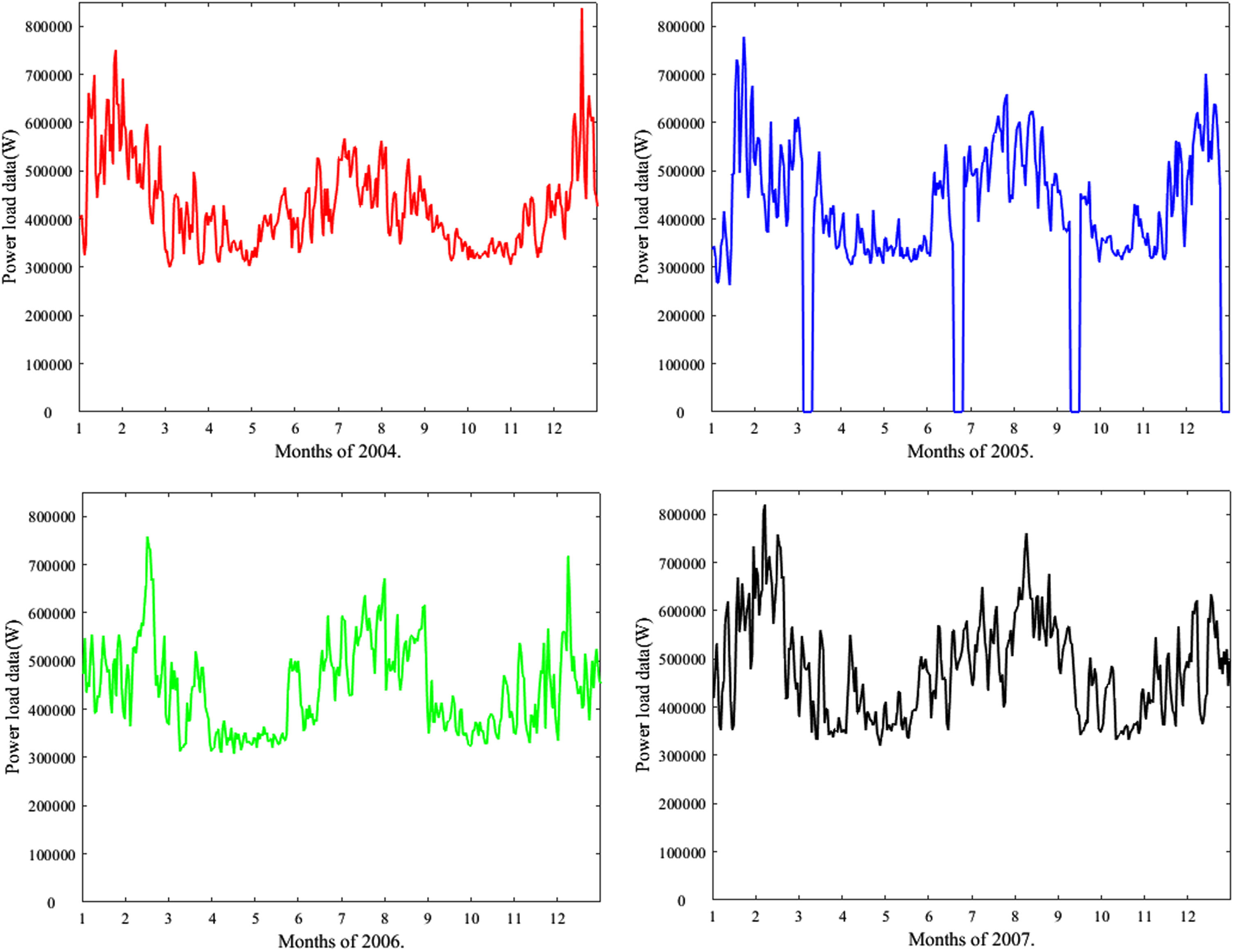
Statistical charts for GEFCom2012 data set.

As shown in Fig. 2, in the GEFCom2012 data set, there is no lack of load data in 2004 and 2007. The load data values of some dates in 2005 and 2006 are 0, and some data show extreme conditions that deviate significantly from other observations. If using this kind of abnormal directly during the experiment, it may have a negative impact on the analysis results, interpretation ability and subsequent prediction results. It is necessary to use data preprocessing and cleaning methods to further process such data to ensure its statistical characteristics and meet the requirements of subsequent load forecasting experiments.

To test the predictive performance of the model, the Mean Absolute Percentage Error (MAPE) and the Mean Absolute Standard Error (MASE) are used in the predictors [28]. The MAPE used to compare the percentage error between the true values and the predicted values, and the smaller the MAPE, the closer the prediction value is to the true value [29]. MASE is a measure of prediction accuracy, whose values range between 0 and 1, and a smaller value of MASE indicates higher prediction accuracy.

The MAPE calculation formula is as follows: $MAPE = \frac{1}{N} \sum_{i = 1}^{N} | \frac{y_{t + i} - \overset{\overset{`}{U}}{y_{t + i}}}{y_{t + i}} | \times 100 %$ (36)

The MASE calculation formula is as follows: $MASE = \frac{1}{N} \sum_{i = 1}^{N} | \frac{y_{t + i} - \overset{\overset{`}{U}}{y_{t + i}}}{\frac{1}{t - 1} \sum_{j = 2}^{t} | y_{j} - y_{j - 1} |} |$ (37)

The predicted value of sample i is y_t+i, and the real value of sample is $\overset{\land}{y_{t + i}}$ .

In order to illustrate the statistical characteristics of the electricity load data provided by the GEFCom2012 data set, descriptive statistics including the mean, standard deviation, maximum value, median, and minimum value were calculated for hourly, daily, and monthly intervals, as shown in Table 1.

Table 1

Statistical features of the GEFCom2012 data set

Time	Intervals	Mean	Std.Dev	Maximum	Median	Minimum
2004	Hourly	23103	5665	39584	23219	9859
	Daily	427065	91223	838313	409709	300048
	Monthly	13025469	2138563	17188825	12262881	10300457
2005	Hourly	18369	5860	40205	16989	7319
	Daily	440858	103918	778296	428090	263530
	Monthly	13519681	2245817	17459083	13353959	10364863
2006	Hourly	18165	5323	39363	17088	8346
	Daily	435968	103918	716679	427799	307836
	Monthly	13384551	2014336	17028928	13097580	10099332
2007	Hourly	19966	6232	45547	159504	9299
	Daily	479174	103783	820200	472415	320925
	Monthly	14575877	2211673	18898480	13977840	11870929

4.1.2 Data preprocessing and outlier cleaning

In order to avoid the impact of missing data on the data analysis process and results, data preprocessing is required before the experiment. Some data have ultra-low values or missing data in the GEFCom2012 data set. If these abnormal data do not have any abnormal description, then such data can be identified as noise data. The generation of such noise data may be due to the planned shutdown of power generation enterprises for maintenance or abnormal external environment, such as extreme natural factors or non-man-made controllable equipment failures, and these noise data must be preprocessed to avoid affecting the results of data analysis and prediction. The data cleaning method for noise data is based on the outlier cleaning method proposed in reference [30], which is improved according to the characteristics of GEFCom2012 data set.

The basic process is as follows, set values that meet the criteria for noisy data as outliers, and replace the outlier values with data generated by specific rules to avoid affecting the experimental results by deleting noisy data directly. The specific method is as follows. Firstly, the original data set is divided into several sub-datasets according to year and month.

The specific method is as follows: first, divide the data set to be analyzed into several subsets based on the same year and month. For example, divide the load data for the year 2004 into 12 subsets according to the months. The subsequent cleaning process will be based on these subsets and remove the data with a load value of 0 in each subset.

Then calculate the average load value for each hour within each subset. Any data within a subset that is less than 1/4 of the average load value will be considered as an outlier.

Afterwards, calculate the weighted average load value for each hour, excluding the outliers. The absolute percentage error (APE) between the hourly load values and the weighted average value is computed. If the calculated APE exceeds 50%, the data point is considered an outlier. Once all the outliers are identified within each subset, the mean interpolation method is used to replace the load data points of these outliers. Specifically, the load data value for an outlier is estimated by taking the weighted average of the corresponding time point for the 7 days before and after the outlier occurrence. ${\bar{y}}_{t}^{v} = \sum_{i = 1}^{7} \frac{(y_{t - i}^{v} \times f_{t - i} + y_{t + i}^{v} \times f_{t + i})}{(f_{t - i} + f_{t + i})}$ (38)

The parameter t in Equation (38) represents the time of the outliers. ${\bar{y}}_{t}^{v}$ is the weighted average of the load values of the outliers, $y_{t + i}^{v}, y_{t - i}^{v}$ represents the load prediction values for seven days before and after the outliers, and f_t-if_t+i is the weight value which is determined based on the distance from the outlier in time and ranges from 1 to 7.

The statistical charts of GEFCom2012 data set after data preprocessing and outlier cleaning are shown in Fig. 3.

Fig. 3

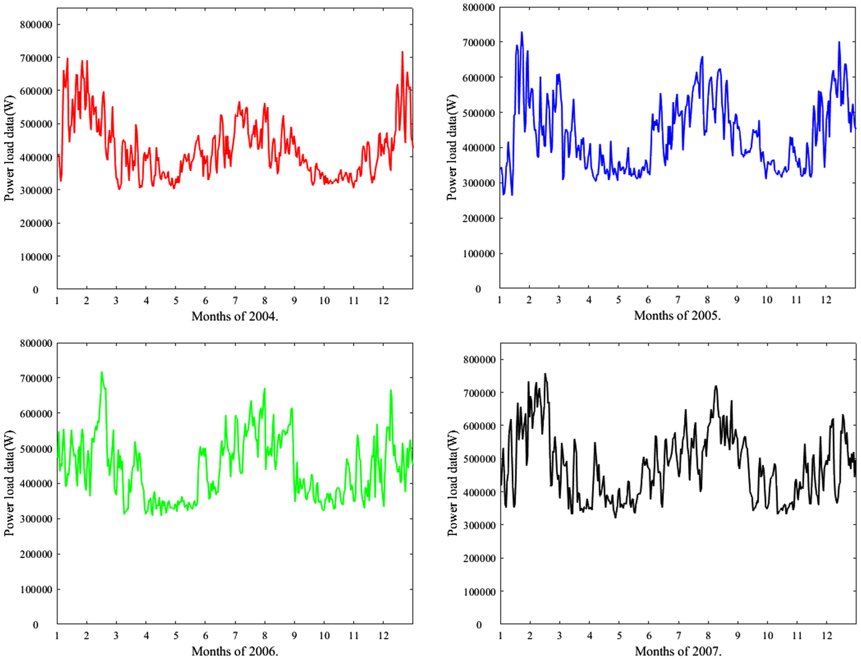
Statistical charts of GEFCom2012 data set after data preprocessing and outlier cleaning.

To avoid overfitting, k-fold cross-validation is used in the experimental process, which can effectively solve the overfitting issue and evaluate the model’s generalization ability, while avoiding uneven division of the training and validation sets. The basic method is to divide the data set into K subsets, select one subset as the validation set each time, and use the remaining K-1 subsets as the training set. Repeat the process K times for cross-validation, and finally use the average of the K metrics as the final model performance measurement. Multiple cross-validations can reduce the impact of randomness on model performance evaluation, make the evaluation results more reliable and stable, and also effectively reduce the risk of model overfitting to training data, while improving the model’s generalization ability and robustness, thus obtaining better performance and predictive power.

After data preprocessing, the data set contains a total of 1,600 records stored on a daily basis from January 1, 2004, to June 29, 2008. Each record consists of 24 hourly power load values, resulting in a total of 38,400 load values. Specifically, there are 362 records for the entire year of 2007, totaling 8,688 load values. The characteristics of the time series and k-fold cross-validation method used in the experiment with the GEFCom2012 data set are not followed according to the common practice of setting the value of k and the number of cross-validation iterations. In the experiment, the data set consisting of 26,016 load values from 2004 to 2006 is used as both the training and validation sets.

After data preprocessing, the GEFCom2012 data set contains a total of 1,600 records stored on a daily basis from January 1, 2004, to June 29, 2008. Each record consists of 24 power load values sampled hourly, resulting in a total of 38,400 load values within these 1,600 records. Specifically, the dataset includes 1,084 records from 2004 to 2006, totaling 26,016 load values used for training and validation. The dataset also includes 362 records from the entire year of 2007, amounting to 8,688 load values used for testing. Due to incomplete data, the 154 records available for the year 2008 are not used in this study.

Each year’s load data is divided into 12 subsets based on the months, and randomly selecting 10 subsets as the training set and the remaining 2 subsets as the validation set. This process will be repeated 10 times for each year to perform cross-validation. For testing purposes, use the load data from the entire year of 2007 consisted of 8,688 load values as the test set.

4.1.3 Input factors and sensitivity analysis

In addition to providing actual electricity load data, the GEFCom2012 data set also includes relevant parameters that influence the electricity load. These parameters primarily consist of load trend variation, temperature data corresponding to time, and holiday data provided according to dates. Considering the impact of temperature and holiday factors on electricity load, these data contribute to constructing more accurate load forecasting models.

Based on the relevant parameters provided by the GEFCom2012 data set, the authors adopt the methodology used in reference [31] with modifications to select input load parameter and conduct sensitivity analysis.

In Table 2, the load parameters combined with their sensitivity weights to obtain the input factors can be used as the calculation parameters of the fuzzy membership function s (x_i), as shown in Equation (39).

Table 2
Load parameters for input factor

Load parameter Notes

Trend A linear trend variable

Tmax Monthly peak temperature

Tt Current hour temperature

Tt-3 Average temperature for the preceding 3 hours and the subsequent 3 hours.

Ta Average temperature of the past 24 hours

Hs Holiday switch, if the date is a holiday then Hs = 1, otherwise Hs = 0

Load parameter	Notes
Trend	A linear trend variable
Tmax	Monthly peak temperature
Tt	Current hour temperature
Tt-3	Average temperature for the preceding 3 hours and the subsequent 3 hours.
Ta	Average temperature of the past 24 hours
Hs	Holiday switch, if the date is a holiday then Hs = 1, otherwise Hs = 0

$\begin{matrix} Factor = θ_{1} Trend \\ + θ_{2} (η_{1} T_{max} + η_{2} T_{t} + η_{3} T_{t - 3} + η_{4} T_{a}) \\ + θ_{3} Hs \\ s . t . θ_{1} + θ_{2} + θ_{3} = 1, η_{1} + η_{2} + η_{3} + η_{4} = 1 \end{matrix}$ (39)

The coefficients θ₁, θ₂, θ₃ and η₁, η₂, η₃, η₄ of the influencing factors have different sensitivities to the load parameters for different values.

According to the analysis in reference [31], it is observed that the trend value coefficient θ₁ should have the highest weight, typically ranging from 0.7 to 0.8, the temperature coefficient θ₂ has a weight range of 0.1 to 0.2, and the holiday coefficient θ₃ is generally set at 0.1. By following the recommendations in references [31], the values will be set as follows: η₁ = 0.05, η₂ = 0.7, η₃ = 0.15, η₄ = 0.1.

Using the historical load data from January to March of 2004 and considering the coefficient ranges and recommended values mentioned earlier, calculate the average MAPE for each day within the monthly range. The result can assess the sensitivity of the parameters θ₁ and θ₂, as shown in Table 3.

Table 3

MAPE values of prediction result

Time	2014.1	2014.2	2014.3
Parameters	MAPE%
θ₁ = 0.7, θ₂ = 0.2	2.73	2.79	2.81
θ₁ = 0.75, θ₂ = 0.15	2.52	2.42	2.58
θ₁ = 0.8, θ₂ = 0.1	2.92	2.99	2.87

Based on the sensitivity analysis of the relevant parameters shown in Table 3, it is observed that a smaller MAPE is achieved when θ₁ = 0.75, θ₂ = 0.15. Based on the analysis process, the coefficient values will be used as θ₁ = 0.75, θ₂ = 0.15, θ₃ = 0.1 and η₁ = 0.05, η₂ = 0.7, η₃ = 0.15, η₄ = 0.1 in Equation (39). In the subsequent experimental process, the input factors determined by multiple load forecasting parameters are calculated using Equation (39). The input factors that affect load forecasting will be introduced into the prediction model through fuzzy membership functions, represented as s (x_i).

4.2 Parameter optimization and experimental steps

4.2.1 Parameter optimization

In the subsequent experimental verification process of the fuzzy support vector regression machine based on boundary vectors, the main optimization parameters include the fuzzy parameter σ, the penalty factor C, and the membership function u_i.

Fuzzy parameter: Control the degree of ambiguity in the fuzzy sample set. In the method proposed in this paper, two parameters of α, β are used to determine the fuzzy parameter.

Penalty factor C: Penalty factor is a parameter that measures the importance of the training model samples. It is used to control the complexity of the model and the degree of fit to the training data.

Membership function u_i: The function of membership function is to evaluate the importance of the sample to the regression plane. The method proposed in this paper does not use the traditional regression plane equation, but uses the minimum hypersphere in the high-dimensional space to determine the membership value of the sample.

In the specific experimental process, it is important to try different combinations of optimization parameters (σ, C and u_i) to find the best configuration, to obtain the best performance and generalization ability of fuzzy support vector regression machine.

As indicated by Equation (19), the product of the penalty factor C and the membership function u_i determines the importance of the sample in the prediction process. The fuzzy parameter σ is determined by α, β. The main optimization parameters selected in the experiment are α, β and C · u_i, and the prediction effect is measured by different optimization combinations of these three parameters.

4.2.2 Experimental procedures

The steps of the power load prediction algorithm based on BVE-FSVR model are as follows:

Step1: Input the data and calculate the values for initial boundary membership function.

Input variables x_i, i = 1, 2, . . . , n of the initial data set and calculate the boundary membership function u (x_i) , i = 1, 2, . . . , n for x_i.

Step2: Calculate fuzzy input variables: Calculate fuzzy input variable m (x_i) and fuzzy membership function s (x_i) = u (m (x_i)) , i = 1, 2, . . . , n using initial data x_i and boundary membership function u (x_i).

Step3: Calculate the fuzzy output variable: Calculate the fuzzy output y_i = f (s (x_i)) , i = 1, 2, . . . , n of x_i based on the calculated m (x_i) and s (x_i).

Step4: Calculate the fuzzy SVR: Train an fuzzy SVR model between the fuzzy input variable m (x_i) and the fuzzy output variable y_i, and obtain the weighting w and bias b based on the training to calculate the SVR fuzzy output $y_{i}^{'} = w \times f (s (x_{i})) + b,$ i = 1, 2, . . . , n of y_i.

Step5: Repeat Step 1 to Step 4 until all the input variables x_i are computed to obtain y_i.

Step6: Defuzzification: Form a set of fuzzy output variables $y_{i}^{'}, i = 1, 2, . . ., n$ obtained from the computation and perform defuzzification to obtain the actual output variable y.

The specific method is as follows: $y = \frac{\sum_{i = 1}^{n} u_{i} \times y_{i}^{'}}{\sum_{i = 1}^{n} u_{i}}, i = 1, 2, . . ., n$ (40)

Step7: Output the Result: Output the obtained actual output variable y as the prediction result.

Take the steps as the basic process, the program flowchart for implementing electricity load forecasting using BVE-FSVR model is shown in Fig. 4.

Fig. 4

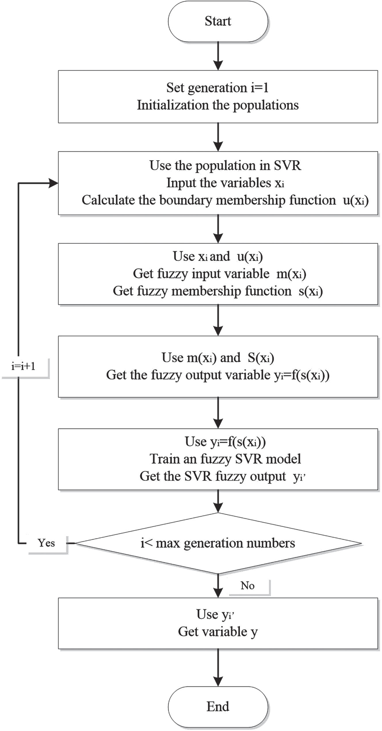
Program flowchart of BVE-FSVR model.

4.3 Experimental process and parameter optimization

4.3.1 Experimental process

The experiment use the power load data provided by GEFCom2012 data set as the training set from the year 2004 to 2006. Using the k-fold validation method divides the load data monthly into 12 subsets for each year, selected 10 random subsets as the training set, and the remaining two subsets are used as the validation set, completed 10 rounds of prediction process and evaluated the prediction results by the values of MAPE and MASE using Equations (36) and (37).

Under the conditions of α+β= 1, experiment select α= 1, β= 0; α= 0.8, β= 0.2; α= 0.6, β= 0.4; α= 0.4, β= 0.6; α= 0.2, β= 0.8; α= 0, β= 1,combined C · u_i = 1, 2, 5 as parameters for training sets. The test data set undergoes 10 rounds of cross-validation using different parameter combinations for each year.

Table 4 and Fig. 5 show the predicted data and schematic diagram obtained for 2004, with different parameters for α, β, C · u_i.

Fig. 5

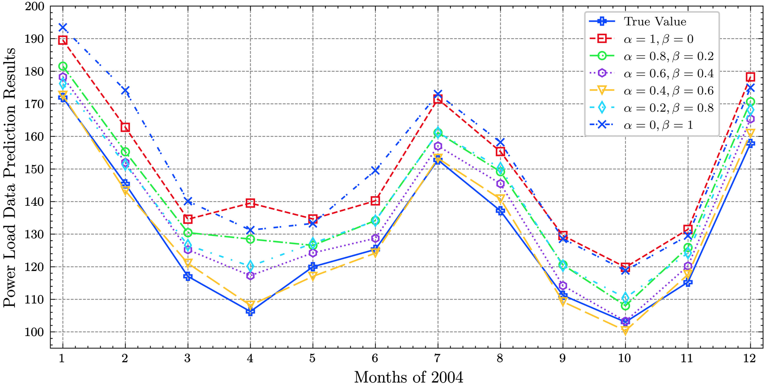
Prediction results used parameters in Table 4.

Table 4

Prediction results with different parameters for 2004

Time	True Value	Predictive value(C · u_i = 1)
		α= 1 β= 0	α= 0.8 β= 0.2	α= 0.6 β= 0.4	α= 0.4 β= 0.6	α= 0.2 β= 0.8	α= 0 β= 1
2004.1	171.89	189.54	181.54	178.26	172.59	176.19	193.45
2004.2	145.40	162.77	155.26	151.98	143.27	151.33	174.12
2004.3	117.04	134.56	130.44	125.21	121.04	126.59	140.11
2004.4	106.24	139.51	128.47	117.25	108.15	120.14	131.23
2004.5	119.97	134.65	126.54	124.23	117.02	127.18	133.27
2004.6	125.29	140.21	134.15	128.71	124.17	134.09	149.55
2004.7	152.76	171.47	161.14	157.05	153.26	161.16	172.98
2004.8	137.15	155.32	149.17	145.48	140.78	150.27	158.21
2004.9	111.22	129.55	120.59	114.18	109.25	120.34	128.55
2004.10	103.00	119.82	108.03	103.27	100.34	110.42	118.81
2004.11	115.26	131.44	125.92	120.22	117.59	124.21	129.53
2004.12	157.83	178.23	170.64	165.37	160.88	168.17	174.94

Table 5 and Fig. 6 show the predicted data and schematic diagram obtained for 2005, with different parameters for α, β, C · u_i.

Fig. 6

Prediction results used parameters in Table 5.

Table 5

Prediction results with different parameters for 2005

Time	True Value	Predictive value(C · u_i = 2)
		α= 1 β= 0	α= 0.8 β= 0.2	α= 0.6 β= 0.4	α= 0.4 β= 0.6	α= 0.2 β= 0.8	α= 0 β= 1
2005.1	147.33	171.44	165.24	154.19	149.25	160.29	173.84
2005.2	135.19	152.37	153.08	140.78	136.48	144.52	159.27
2005.3	137.95	158.91	149.77	142.33	133.92	146.38	151.30
2005.4	103.65	134.78	123.05	113.81	106.24	119.91	128.64
2005.5	104.62	130.55	128.99	115.97	106.04	112.12	127.82
2005.6	130.41	150.09	145.62	134.06	128.57	141.83	154.24
2005.7	163.64	175.91	170.29	160.08	156.71	166.66	179.60
2005.8	162.25	184.88	178.51	169.24	160.27	167.37	177.08
2005.9	131.89	144.62	140.39	136.43	129.79	138.05	149.48
2005.10	109.99	131.37	124.82	112.02	107.51	118.40	133.76
2005.11	120.86	142.48	167.74	128.67	123.92	132.57	141.87
2004.12	157.83	178.23	170.64	165.37	160.88	168.17	174.94

Table 6 and Fig. 7 show the predicted data and schematic diagram obtained for 2006, with different parameters for α, β, C · u_i.

Table 6

Prediction results with different parameters for 2006

Time	True Value	Predictive value(C · u_i = 5)
		α= 1 β= 0	α= 0.8 β= 0.2	α= 0.6 β= 0.4	α= 0.4 β= 0.6	α= 0.2 β= 0.8	α= 0 β= 1
2006.1	145.56	167.22	163.94	157.92	151.15	159.07	170.25
2006.2	142.40	168.75	162.77	155.01	148.06	157.22	168.64
2006.3	128.08	141.18	136.19	129.35	120.54	131.60	144.83
2006.4	100.99	129.94	120.98	114.62	107.52	118.37	132.72
2006.5	114.64	101.37	103.47	105.84	108.92	120.46	130.95
2006.6	133.87	161.81	153.47	146.28	140.73	152.31	167.02
2006.7	170.29	194.93	186.05	182.67	176.64	180.16	187.81
2006.8	162.56	188.86	182.04	177.41	169.54	176.29	185.73
2006.9	113.06	130.84	123.95	115.83	109.82	127.05	130.07
2006.10	116.64	140.97	131.73	127.42	122.48	131.48	143.70
2006.11	127.99	151.27	140.36	129.18	119.35	127.83	138.13
2006.12	150.04	170.89	160.77	153.21	145.98	161.01	178.90

Fig. 7

Prediction results used parameters in Table 6.

Based on the experimental process and results obtained in this section, the values of MAPE and MASE have been calculated using Equations (36) and (37) that as shown in Table 7. Based on the analysis of Table 4, it can be observed that when α= 0.4, β= 0.6 and C · u_i = 1 or C · u_i = 2, the values of MAPE and MASE for prediction results from 2004 to 2006 are smallest among all parameter combinations. This analysis result indicates that choosing this parameter combination can achieve higher prediction accuracy, and the subsequent parameter optimization process will focus on the range of parameter values around combination.

Table 7

Values of MAPE and MASE for different parameter combinations

Time	2014.1–2014.12		2015.1–2015.12		2016.1–2016.12
C · u_i	1		2		5
Parameter	MAPE%	MASE	MAPE%	MASE	MAPE%	MASE
α= 1,β= 0	1.775	0.441	1.698	0.407	2.305	0.607
α= 0.8,β= 0.2	1.663	0.305	1.574	0.289	2.224	0.462
α= 0.6,β= 0.4	1.651	0.231	1.551	0.274	2.179	0.433
α= 0.4,β= 0.6	1.607	0.209	1.473	0.261	2.011	0.415
α= 0.2,β= 0.8	1.781	0.377	1.492	0.330	2.253	0.541
α= 0,β= 1	1.920	0.591	1.605	0.415	2.506	0.688

4.3.2 Parameter optimization

Considering the experimental results in section 4.3.1, when α= 0.4, β= 0.6, and the value of C · u_i is around 1 or 2, the prediction accuracy is relatively higher. Based on the research findings, the K-fold cross-validation method will be used to perform parameter optimization again for load forecasting from 2004 to 2006. Five sets of parameters are selected: α= 0.6, β= 0.4; α= 0.5, β= 0.5; α= 0.4, β= 0.6; α= 0.3, β= 0.7; α= 0.2, β= 0.8. The parameter value for C · u_i is chosen as 1, 1.5, and 2. The existing prediction results obtained using the same parameters will be preserved, and the new parameter combinations will undergo 10 rounds of training and validation to obtain the average results for load prediction.

Table 8 and Fig. 8 show the predicted data and schematic diagram obtained for 2004 with different parameters for α, β, C · u_i.

Table 8
Prediction results with different parameters for 2004

Time True Value Predictive value(C · u_i = 1)

α= 0.6 β= 0.4 α= 0.5 β= 0.5 α= 0.4 β= 0.6 α= 0.3 β= 0.7 α= 0.2 β= 0.8

2004.1 171.89 178.26 176.21 172.59 172.26 176.19

2004.2 145.40 151.98 148.96 143.27 144.31 151.33

2004.3 117.04 125.21 124.58 121.04 120.62 126.59

2004.4 106.24 117.25 114.38 109.15 108.07 120.14

2004.5 119.97 124.23 123.20 117.02 120.67 127.18

2004.6 125.29 128.71 127.31 124.17 123.94 134.09

2004.7 152.76 157.05 156.26 153.26 151.16 161.16

2004.8 137.15 145.48 143.68 140.78 139.95 150.27

2004.9 111.22 114.18 113.26 109.25 110.33 120.34

2004.10 103.00 103.27 102.19 100.34 104.92 110.42

2004.11 115.26 120.22 118.64 117.59 114.02 124.21

2004.12 157.83 165.36 163.17 160.88 155.77 168.17

Time	True Value	Predictive value(C · u_i = 1)
		α= 0.6 β= 0.4	α= 0.5 β= 0.5	α= 0.4 β= 0.6	α= 0.3 β= 0.7	α= 0.2 β= 0.8
2004.1	171.89	178.26	176.21	172.59	172.26	176.19
2004.2	145.40	151.98	148.96	143.27	144.31	151.33
2004.3	117.04	125.21	124.58	121.04	120.62	126.59
2004.4	106.24	117.25	114.38	109.15	108.07	120.14
2004.5	119.97	124.23	123.20	117.02	120.67	127.18
2004.6	125.29	128.71	127.31	124.17	123.94	134.09
2004.7	152.76	157.05	156.26	153.26	151.16	161.16
2004.8	137.15	145.48	143.68	140.78	139.95	150.27
2004.9	111.22	114.18	113.26	109.25	110.33	120.34
2004.10	103.00	103.27	102.19	100.34	104.92	110.42
2004.11	115.26	120.22	118.64	117.59	114.02	124.21
2004.12	157.83	165.36	163.17	160.88	155.77	168.17

Fig. 8

Prediction results used parameters in Table 8.

Table 9 and Fig. 9 show the predicted data and schematic diagram obtained for 2005 with different parameters for α, β, C · u_i.

Table 9

Prediction results with different parameters for 2005

Time	True Value	Predictive value(C · u_i = 1.5)
		α= 0.6 β= 0.4	α= 0.5 β= 0.5	α= 0.4 β= 0.6	α= 0.3 β= 0.7	α= 0.2 β= 0.8
2005.1	147.33	156.01	150.99	148.07	146.98	158.33
2005.2	135.19	144.78	140.17	137.05	134.77	149.26
2005.3	137.95	141.02	140.05	139.21	138.24	143.19
2005.4	103.65	117.26	110.32	105.33	104.08	116.08
2005.5	104.62	118.30	111.28	106.01	105.20	114.02
2005.6	130.41	139.26	130.45	127.91	131.10	142.07
2005.7	163.64	173.21	170.26	165.70	162.17	173.24
2005.8	162.25	173.80	167.37	164.08	163.27	170.01
2005.9	131.89	140.07	137.30	132.65	130.94	142.40
2005.10	109.99	117.04	111.84	106.37	108.21	117.54
2005.11	120.86	130.09	124.90	118.04	121.28	130.21
2005.12	174.59	186.70	178.55	171.11	172.08	185.04

Fig. 9

Prediction results used parameters in Table 9.

Table 10 and Fig. 10 show the predicted data and schematic diagram obtained for 2006 with different parameters for α, β, C · u_i.

Table 10

Prediction results with different parameters for 2006

Time	True Value	Predictive value(C · u_i = 2)
		α= 0.6 β= 0.4	α= 0.5 β= 0.5	α= 0.4 β= 0.6	α= 0.3 β= 0.7	α= 0.2 β= 0.8
2006.1	145.56	151.77	150.85	148.27	147.51	153.58
2006.2	142.40	148.25	146.81	145.26	140.32	150.27
2006.3	128.08	136.54	135.54	133.29	130.77	139.80
2006.4	100.99	108.75	106.92	103.82	97.04	110.45
2006.5	114.64	120.39	118.79	115.88	111.31	123.24
2006.6	133.87	146.52	145.14	140.71	135.63	148.17
2006.7	170.29	179.28	178.87	176.14	173.84	181.93
2006.8	162.56	170.84	168.52	166.25	165.10	172.25
2006.9	113.06	118.71	117.80	114.43	110.92	119.62
2006.10	116.64	127.62	126.93	124.50	119.06	126.31
2006.11	127.99	137.80	134.69	128.21	124.78	140.54
2006.12	150.04	160.23	157.44	156.30	153.11	163.17

Fig. 10

Prediction results used parameters in Table 10.

Based on the completed parameter optimization process, it is evident that when using the parameter combination α= 0.3, β= 0.7and C · u_i = 1.5, the predicted values obtained from the BVE-FSVR model are closest to the actual load values. By calculating the MAPE and MASE values from 2004 to 2006 as evaluation metrics for prediction accuracy, it can be concluded that the parameter combination α= 0.3, β= 0.7and C · u_i = 1.5 achieves the highest prediction accuracy. Therefore, this parameter combination will be used in the subsequent prediction process on the test set. The specific prediction accuracy indicators are shown in Table 11.

Table 11

Values of MAPE and MASE for different parameter combinations

Time	2004.1–2004.12		2005.1–2005.12		2006.1–2006.12
C · u_i	1		1.5		2
Parameter	MAPE%	MASE	MAPE%	MASE	MAPE%	MASE
α= 0.6,β= 0.4	1.651	0.231	1.504	0.221	1.573	0.285
α= 0.5,β= 0.5	1.643	0.229	1.478	0.217	1.570	0.281
α= 0.4,β= 0.6	1.607	0.209	1.450	0.205	1.495	0.266
α= 0.3,β= 0.7	1.549	0.193	1.402	0.195	1.479	0.252
α= 0.2,β= 0.8	1.781	0.377	1.588	0.206	1.632	0.327

Fig. 11

Comparison of power load data prediction results obtained using different machine learning models.

4.4 Predicted results analysis

To evaluate the performance of BVE-FSVR method in power load forecasting, in conjunction with the results obtained in the previous experimental process, the BVE-FSVR method selects α= 0.3, β= 0.7, and C · u_i= 1.5 as the parameters for the test set. The electricity load data for the 12 months of the year 2007 from the GEFCom2012 data set is used as the test set. In order to compare the differences between the proposed FSVR method and other machine learning models, several machine learning models commonly used for power load forecasting, including SVM, SVR, BPNN, and ABC are implemented for load prediction.

The experimental parameters for each method in the experiment process were referenced from recent relevant literature for the basic methods and parameter values [32–35], as shown in Table 12, and the specific prediction results are shown in Table 13 and Fig. 10.

Table 12
Parameter values used different prediction models

Model Parameters Values Notes

SVM C = 10 Penalty factor

RBF Kernel function type

γ= 0.1 The parameter of RBF kernel function.

SVR C=10 Penalty factor

ɛ= 0.01 Determine the acceptable error range.

RBF Kernel function type.

γ= 0.1 The parameter of RBF kernel function.

BPNN α= 0.1 Determine the learning rate.

N = 100 Number of processing units

Sigmoid Determine activation conditions.

I = 50 Number of times the entire training data set

B = 128 Number of training examples

λ= 0.01 Control the degree of regularization

ABC B = 200 Number of bees in the search space.

I = 100 Maximum number of iterations executes.

N = 10 The range that bees search for solutions.

E = 30 The number of best solutions

S = 100 The number of bees in each iteration.

U = 0.5 Control the update speed of bee positions.

W = 0.1 Control the weight of objective function.

Model	Parameters Values	Notes
SVM	C = 10	Penalty factor
	RBF	Kernel function type
	γ= 0.1	The parameter of RBF kernel function.
SVR	C=10	Penalty factor
	ɛ= 0.01	Determine the acceptable error range.
	RBF	Kernel function type.
	γ= 0.1	The parameter of RBF kernel function.
BPNN	α= 0.1	Determine the learning rate.
	N = 100	Number of processing units
	Sigmoid	Determine activation conditions.
	I = 50	Number of times the entire training data set
	B = 128	Number of training examples
	λ= 0.01	Control the degree of regularization
ABC	B = 200	Number of bees in the search space.
	I = 100	Maximum number of iterations executes.
	N = 10	The range that bees search for solutions.
	E = 30	The number of best solutions
	S = 100	The number of bees in each iteration.
	U = 0.5	Control the update speed of bee positions.
	W = 0.1	Control the weight of objective function.

Table 13

Prediction results using different machine learning models

Time	True Value	BVE-FSVR	SVM	SVR	BPNN	ABC
2007.1	164.59	167.41	173.51	169.32	168.04	172.45
2007.2	173.31	179.45	185.47	184.14	170.54	185.98
2007.3	128.94	127.84	130.25	131.54	130.47	135.58
2007.4	118.71	120.74	125.41	109.25	117.45	129.54
2007.5	124.28	126.21	117.22	129.14	128.56	134.78
2007.6	145.38	147.84	150.34	151.21	160.25	160.22
2007.7	161.44	163.51	167.11	160.25	171.24	167.44
2007.8	188.98	185.21	190.84	178.19	184.21	190.84
2007.9	134.18	136.87	136.17	140.23	139.52	137.45
2007.10	118.94	119.05	128.10	111.54	127.25	139.52
2007.11	132.65	133.97	138.42	139.12	136.45	132.74
2007.12	157.57	156.98	168.80	160.25	161.84	164.11

In Table 14, the values of MAPE and MASE are recorded for the different prediction models using the electricity load data of 2007 that provided by the GEFCom2012 data set.

Table 14

Values of MAPE and MASE for different prediction models

Prediction Model	MAPE%	MASE
SVM	1.809	0.278
SVR	1.732	0.254
BPNN	2.774	0.541
ABC	2.270	0.422
BVE-FSVR	1.585	0.227

Based on the comparison of the predicted results and the MAPE and MASE values, it can be concluded that when comparing the SVM, SVR, BPNN, ABC, and BVE-FSVR methods as load forecasting models, the BVE-FSVR method demonstrates significantly higher predictive accuracy and result stability than the BPNN and ABC methods, and slightly higher than the SVR and SVM methods.

Based on the above analysis results and considering the design principles and methods commonly used in machine learning models for electricity load forecasting, an analysis result can be obtained through comparison and summarization of these methods. SVM can handle high-dimensional and nonlinear data, has good generalization ability, and is robust in handling outliers. However, its predictive results may not be highly interpretable. SVR can handle nonlinear relationships and high-dimensional data, has good generalization ability and robustness, but is sensitive to hyperparameter selection. BPNN can capture nonlinear relationships in the data, has good adaptability and generalization ability, but it is prone to being trapped in local optima and requires significant computational resources during training. ABC has the ability for global search and can avoid being stuck in local optima, but its performance significantly declines when dealing with high-dimensional problems. Compared to these methods, the proposed approach in this paper demonstrates higher prediction accuracy and stability in power load forecasting. It is suitable for handling nonlinear relationships and high-dimensional data, shows good robustness against outliers, and has the ability to provide real-time predictions with integration capabilities for big data analysis.

5 Conclusion

In this paper, the authors proposed an improved fuzzy support vector regression (FSVR) algorithm to enhance the accuracy of power load forecasting. Authors applied the boundary membership function to the typical FSVR algorithm and incorporated boundary and distance factors into the design of the membership function. The proposed method has been using GEFCom2012 data set, and trained and validated the algorithm model using a subset of the prediction data set, obtaining the optimal parameter combination. The predicted results compared with algorithm models generated by commonly used methods such as BP Neural Network, Artificial Bee Colony, SVR, and SVM. The prediction results demonstrated that the BVE-FSVR method outperformed the BP Neural Network and Artificial Bee Colony models significantly and slightly outperformed the SVR and SVM models in terms of prediction accuracy.

The power load forecasting method proposed in this paper has wide applications in power enterprises, including the combination strategy of power generation units, design of power transmission schemes between different regions, and power load scheduling and operation. This method can effectively improve the operational economy of the power system, and the predicted results can serve as important reference for power system dispatch, production planning, and electricity planning and design.

In the future, the development of power load forecasting will trend towards more prediction that is refined, real-time interaction, and integration with big data analysis and processing. BVE-FSVR method proposed in this paper demonstrates high levels of prediction accuracy and stability. Therefore, transforming the method proposed in this paper into a program model suitable for typical real-time big data analysis platforms will be the direction for future development and research.

Footnotes

Acknowledgments

This work was supported by Applied Basic Research Program of Liaoning Province, China.

Grant: [2022JH2/101300134], [2023JH2/101300065].

References

Yinsheng

, et al., Principal Component Analysis of Short-term Electric Load Forecast Data Based on Grey Forecast, Journal of Physics Conference Series 1486 (2020), 062031.

Elbaz

Khalid

, et al., Prediction of Disc Cutter Life during Shield Tunneling with AI via the Incorporation of a Genetic Algorithm into a GMDH-Type Neural Network, Engineering 7. prepublish (2020).

Mohamed

Shaban Wafaa

, et al., A multi-objective optimization algorithm for forecasting the compressive strength of RAC with pozzolanic materials, Journal of Cleaner Production 327 (2021).

Tao

Yan

, et al., Prediction of long-term water quality using machine learning enhanced by Bayesian optimisation, (Barking, Essex: 1987) 318 (2022). Elbaz Khalid, et al., Spatiotemporal air quality forecasting and health risk assessment over smart city of NEOM, Chemosphere (2022).

YuLin

Chen

, ShuiLong

Shen

and Annan

Zhou

, Assessment of red tide risk by integrating CRITIC weight method, TOPSIS-ASSETS method, and Monte Carlo simulation, Environmental Pollution (Barking, Essex: 1987), 314 (2022).

Cun-Yong

Qiu

and Jian

, Power System Short-Term Load Forecasting Based on Support Vector Regression, Computer Simulation (2013).

Cortes

Corinna

and Vapnik

, Support-Vector Networks, Machine Learning 20(3) (1995), 273–297.

Guo-Feng

Fan

, et al., Forecasting short-term electricity load using hybrid support vector regression with grey catastrophe and random forest modeling, Utilities Policy 73 (2021).

Rui

Wang

, et al., Corrigendum: Clifford Fuzzy Support Vector Machine for Regression and Its Application in Electric Load Forecasting of Energy System, Frontiers in Energy Research (2022).

10.

Weiguo

Zhang

, et al., A hybrid SVR with the firefly algorithm enhanced by a logarithmic spiral for electric load forecasting, Frontiers in Energy Research (2022).

11.

Jian

Luo

, et al., A robust support vector regression model for electric load forecasting, International Journal of Forecasting 39(2) (2023).

12.

Balasundaram

and Prasad

Subhash Chandra

, Robust twin support vector regression based on Huber loss function, Neural Computing and Applications 32(15) (2019).

13.

Chih-Chung , et al., LIBSVM: A library for support vector machines, Acm Transactions on Intelligent Systems & Technology (2011).

14.

Sriwastava

Brijesh

, Basu

and Maulik

, Predicting Protein-Protein Interaction Sites with a Novel Membership Based Fuzzy SVM Classifier, IEEE/ACM Transactions on Computational Biology & Bioinformatics 12(6) (2015), 1394–1404.

15.

Banghan

, et al., Research on load forecasting method of large Power Grid based on Deep confidence Network, IOP Conference Series: Earth and Environmental Science.

16.

Gupta

Deepak

and Gupta

, On robust asymmetric Lagrangian ν-twin support vector regression using pinball loss function, Applied Soft Computing 102(3) (2021), 107099.

17.

Wahba

Grace

, Support Vector Machines, Reproducing Kernel Hilbert Spaces and the Randomized GACV, MIT Press (1998).

18.

Jumutc

Vilen

, Huang

and Suykens

J.A.K.

, Fixed-size Pegasos for hinge and pinball loss SVM, IJCNN IEEE, 2013.

19.

Huang

Xiaolin

, et al., Support Vector Machine Classifier With Pinball Loss, Pattern Analysis and Machine Intelligence (2014).

20.

Zhang

Zhaoxiong

, Surtemperature prediction model of continuous casting slab based on Svector principle, Chinese Science and Technology Iinformation 6 (2016), 54–55.

21.

Sriwastava

Brijesh K.

, et al., Predicting Protein-Protein Interaction Sites with a Novel Membership Based Fuzzy SVM Classifier, IEEE/ACM Transactions on Computational Biology and Bioinformatics (TCBB) 12(6) (2015).

22.

Lin

C.F.

and Wang

S.D.

, Fuzzy support vector machines[J], IEEE Transactions on Neural Networks 13(2) (2002), 464–471.

23.

Jian

, Niu

, Xia

, Samir

, Sumanasekera

, Mu

, Jennings

J.L.

, Hoek

K.L.

, Allos

, Howard

L.M.

et al., A novel algorithm for validating peptide identification from a shotgun proteomics search engine, J Proteome Res 12(3) (2013), 1108–1119.

24.

Chang

C.-C.

et al., Libsvm: A library for support vector machines, ACM Trans Intell Syst Technol 2(3) (2011), 1–27.

25.

Everett

L.J.

, Bierl

and Master

S.R.

, Unbiased statistical analysis for multi-stage proteomic search strategies, J Proteome Res, 9(2) (2010), 700–707.

26.

Weng

Yongqiang

, Wu

Chunshan

, Jiang

Qiaowei

, Guo

Wenming

, Wang

Cong

. Application of support vector machines in medical data[C], Proceedings of 2016 4th IEEE International Conference on Cloud Computing and Intelligence Systems, (IEEE CCIS:2016), (2016), 227–231.

27.

Hong

Tao

, Pinson

and Fan

, Global Energy Forecasting Competition, International Journal of Forecasting 30(2) (2014), 357–363.

28.

Liantoni

Febri

and Agusti

Arif

, Forecasting Bitcoin using Double Exponential Smoothing Method Based on Mean Absolute Percentage Error, JOIV International Journal on Informatics Visualization 4(2) (2020).

29.

Maiseli

Baraka Jacob

, Optimum design of chamfer masks using symmetric mean absolute percentage error, EURASIP Journal on Image and Video Processing 2019(1) (2019).

30.

Xie

Jingrui

and Hong

, GEFCom2014 probabilistic electric load forecasting: An integrated solution with forecast combination and residual simulation, International Journal of Forecasting 32(3) (2016), 1012–1016.

31.

Hong

Tao

, Wang

and Willis

H.L.

, A Naïve multiple linear regression benchmark for short term load forecasting, IEEE Power & Energy Society General Meeting IEEE, 2011.

32.

Yibing

Shao

, Xiaofen

, Menglin

Zheng

and Caiya

Chen

, Prediction of Standard Time of the Sewing Process using a Support Vector Machine with Particle Swarm Optimization[J], Autex Research Journal 22(3) (2021).

33.

Lin

and Liu

Zuoming

, Short-term Power Load Forecasting Based on Optimized Support Vector Regression[C], Proceedings of 2018 3rd International Conference on Industrial Electronics and Applications (IEA 2018), Information Engineering Research Institute, 2018:24–28.

34.

Kang

et al., Short-Term Load Forecasting of Power System Based on WT-IPSO-BPNN, Electrical Engineering Technology (2021).

35.

et al., Short-term Power Load Forecasting Based on Improved ABC and IDPC-MKELM, Smart Grid 009 (2022), 050.