Minimizing fuzzy makespan in a distributed assembly flow shop by using an efficient artificial bee colony algorithm

Abstract

Assembly flow shop scheduling problem (AFSP) in a single factory has attracted widespread attention over the past decades; however, the distributed AFSP with DPm → 1 layout considering uncertainty is seldom investigated. In this study, a distributed assembly flow shop scheduling problem with fuzzy makespan minimization (FDAFSP) is considered, and an efficient artificial bee colony algorithm (EABC) is proposed. In EABC, an adaptive population division method based on evolutionary quality of subpopulation is presented; a competitive employed bee phase and a novel onlooker bee phase are constructed, in which diversified combinations of global search and multiple neighborhood search are executed; the historical optimization data set and a new scout bee phase are adopted. The proposed EABC is verified on 50 instances from the literature and compared with some state-of-the-art algorithms. Computational results demonstrate that EABC performs better than the comparative algorithms on over 74% instances.

Keywords

distributed assembly flow shop scheduling uncertainty artificial bee colony algorithm fuzzy makespan

1 Introduction

Assembly shop scheduling problem plays an essential role in balancing batch production and production flexibility. It has been widely used in many manufacturing industries such as fire engine [1], computer [2], clothes [3] and automobiles [4]. Facing the competitive market, research on assembly shop scheduling can assist managers to choose an efficient scheduling plan and help enterprises produce more products in the shortest time. Relevant problems have been considered and a large number of results have been obtained since the pioneering work of Lee et al. [1]. After that, a unified definition method and a full review of assembly scheduling problems were displayed by Framinan et al. [5] and Komaki et al. [6].

As a frequently investigated problem, AFSP has been successfully studied, and most works are about AFSP with DPm → 1 layout, which consists of m dedicated parallel machines and an assembly machine. For AFSP in a single factory, various meta-heuristics have been the main optimization method. Allahverdi and Al-Anzi [7] first introduced tabu search and particle swarm optimization(PSO) algorithm to handle AFSP with makespan criterion in 2006. Wu et al. [8] studied the problem through a branch-and-bound algorithm and six hybrid PSO algorithms. Shokrollahpour et al. [9] presented an imperialist competitive algorithm (ICA) to minimize the weighted sum of mean completion time and makespan in AFSP. Kazemi et al. [10] developed a hybrid ICA incorporating a dominant relation for AFSP with batching and delivery. Considering setup times, Mozdgir et al. [11] proposed three meta-heuristics: differential evolution algorithm, genetic algorithm(GA) and population-based variable neighborhood search algorithm to minimize makespan in no-wait AFSP. Jung et al. [12] provided three versions of genetic algorithm (GA) to obtain minimum makespan in AFSP with dynamic component-sizes. Basir et al. [13] also applied a bi-level GA to the problem with batch delivery systems. Afterward, Komaki et al. [14] proved the effectiveness of a discrete cuckoo optimization algorithm in solving the three-stage AFSP with makespan minimization. In addition, Azzouz et al. [15] devised a hybrid greedy iterative algorithm on AFSP with small and big size jobs. More detailed meta-heuristic algorithms on AFSP can be found in [16].

The above works on AFSP are all accomplished in a single factory. Nowadays, production and scheduling are gradually transforming from a single factory to multiple factories to respond quickly to the changes in market demand. Different from AFSP in a single factory, distributed assembly flow shop scheduling problem (DAFSP) reveals more sub-problems and more complex interrelationships among subproblems.

Regarding DAFSP with DPm → 1 layout in each factory, Xiong et al. [17] established a variable neighborhood search algorithm (VNS) and a hybrid variable neighborhood search algorithm combined with reduced variable neighborhood search (GA-RVNS) to minimize the time-related objective. Deng et al. [18] applied a competitive memetic algorithm (CMA) to solve the problem with makespan optimization. Lei et al. [19] provided a cooperated teaching-learning-based optimization algorithm to investigate the problem with makespan criterion. Li et al. [20] developed an imperialist competitive algorithm with empire cooperation (ECICA) to minimize the fuzzy makespan.

Besides that, other types of DAFSP are also considered. For DAFSP consisting of F manufacturing factories and one assembly factory, Hatami et al. [21] designed a variable neighborhood descent algorithm to minimize makespan. Wang et al. [22] proposed a novel memetic algorithm to optimize the maximum completion time. Lin et al. [23] presented a backtracking search hyper-heuristic algorithm to obtain the minimum makespan. Sang et al.[24] provided an effective invasive weed optimization algorithm to optimize total flow time. Huang et al. [25] reported an iterated greedy algorithm for the same problem. Zhao et al. [26] also investigated a self-learning hyper-her-heuristic to minimize the total flow time. Wang et al. [27] presented a cooperative memetic algorithm with feedback to minimize total tardiness and energy consumption. Zhang et al. [28] proposed a matrix cube-based estimation of distribution algorithm to minimize the makespan and total carbon emission. For DAFSP with F factories containing a flow shop and an assembly line in each factory, Pan et al. [29] utilized three heuristics, two VNS and an iterated greedy algorithm to minimize makespan.

As stated above, FDAFSP has attracted much attention. However, research on DAFSP with DPm → 1 layout is limited, and DAFSP with uncertainty is seldom investigated. Moreover, various uncertain factors extensively exist in the actual processing environment, and the negligence of uncertainty may invalidate the original scheduling plan. In recent years, the fuzzy set theory [30] has been widely used to solve fuzzy scheduling problems [31 –37]. According to the definition of fuzzy dimension [38, 39], the fuzzy dimension of FDAFSP is decided by the number of processed jobs, and operations on fuzzy numbers also can be applied to the research of FDAFSP. Therefore, it is significant to investigate FDAFSP.

Various meta-heuristic algorithms [15–18 , 41] own excellent optimization performance and have been used to deal with multi-domain problems including AFSP and DAFSP. Compared with other meta-heuristics, artificial bee colony algorithm (ABC) [42, 43] has certain characteristics, such as simple algorithm structure, fast convergence speed and effective global search ability [44 –46]; on the other hand, ABC shows excellent abilities and advantages in solving production scheduling in a single factory [47 –50] and multiple factories [51 –53]. However, ABC has not been applied to cope with DAFSP, let alone FDAFSP. Thus, we are motivated to improve ABC for solving FDAFSP.

The contributions of this study can be concluded as follows: (1) FDAFSP with DPm → 1 layout in each factory is considered and a novel algorithm called EABC is proposed to minimize fuzzy makespan. (2) In EABC, an adaptive population division procedure based on evolutionary quality of subpopulation is implemented; the newly designed employed bee phase and onlooker bee phase are performed by utilizing a diversified combinations of global search and multiple neighborhood search; historical data set and a novel scout bee phase are constructed. (3)A number of comparative experiments are conducted to test the performance of EABC on the considered FDAFSP. Computational results demonstrate that EABC holds more advantages than other algorithms on over 74% instances.

The rest of this article is structured as follows. Fuzzy operations are shown in Section 2, and the problem description is given in Section 3. Section 4 reports EABC for FDAFSP and is followed by the computational results in Section 5. Conclusions and future research topics are summarized in the final section.

2 Operations on fuzzy processing time

Due to its convenience, triangular fuzzy number(TFN) is often adopted to describe fuzzy processing time in shop scheduling problem [31 –37]. A TFN can be expressed as $\tilde{t} = (t_{1}, t_{2}, t_{3})$ , where an interval value [t₁, t₃] contains the possible values and t₂ ∈ [t₁, t₃] is a modal value.

In this article, the fuzzy processing, setup and assembly time are all expressed as TFNs. Three operators, including addition, ranking and max, are provided to build a scheduling. Addition is applied to compute the completion time of jobs. Ranking is used to make a comparison between fuzzy objectives. Max is utilized to calculate the fuzzy beginning time of jobs.

For TFNs $\tilde{a} = (a_{1}, a_{2}, a_{3})$ and $\tilde{b} = (b_{1}, b_{2}, b_{3})$ , addition operation is conducted by $\tilde{a} + \tilde{b} = (a_{1} + b_{1}, a_{2} + b_{2}, a_{3} + b_{3})$ (1)

For $\tilde{a}$ , $Z_{1} (\tilde{a}) = (a_{1} + 2 a_{2} + a_{3}) / 4$ , $Z_{2} (\tilde{a}) = a_{2}$ , $Z_{3} (\tilde{a}) = a_{3} - a_{1}$ .

Ranking $\tilde{a}$ and $\tilde{b}$ is realized through the following conditions:

If $Z_{1} (\tilde{a}) > Z_{1} (\tilde{b})$ or $Z_{1} (\tilde{a}) = Z_{1} (\tilde{b})$ , and $Z_{2} (\tilde{a}) > Z_{2} (\tilde{b})$ or $Z_{i} (\tilde{a}) = Z_{i} (\tilde{b})$ , i = 1, 2 and $Z_{3} (\tilde{a}) > Z_{3} (\tilde{b})$ , then $\tilde{a} > \tilde{b}$ .

Max operation is implemented in terms of $\tilde{a} \lor \tilde{b}$ , which is defined by an effective approximation criterion: $\tilde{a} \lor \tilde{b} ≃ (a_{1} \lor b_{1}, a_{2} \lor b_{2}, a_{3} \lor b_{3})$ (2)

3 The definition of the problem

FDAFSP consists of n jobs {J₁, J₂, ⋯ , J_n } and f homogeneous factories {F₁, F₂, ⋯ , F_f } distributed in different sites. Each factory f possesses m dedicated parallel machines M_f1, M_f2, ⋯ , M_fm at the fabrication stage and one assembly machine AM_f at the assembly stage. Each job is composed of m components, which are first processed on m manufacturing machines, then transported to AM_f and assembled together into a final product. Figure 1 shows an illustration of FDAFSP.

Fig. 1

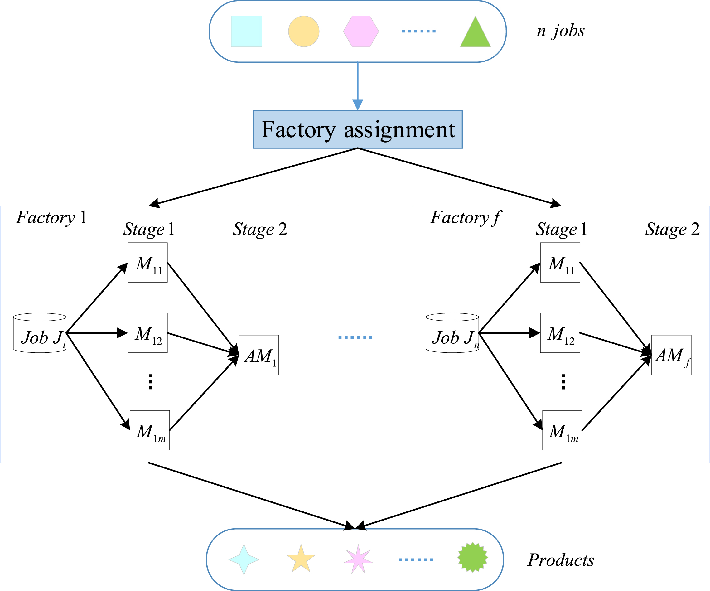
an illustration of FDAFSP.

Jobs in each factory have same setup, processing and assembly time. At fabrication stage, fuzzy setup and processing time of job J_i on machine M_fk are ${\tilde{s}}_{ik} = (s_{ik}^{1}, s_{ik}^{2}, s_{ik}^{3})$ and ${\tilde{p}}_{ik} = (p_{ik}^{1}, p_{ik}^{2}, p_{ik}^{3})$ . At assembly stage, fuzzy adjustment and assembly time of job J_i on AM_f are expressed by ${\tilde{u}}_{i} = (u_{i}^{1}, u_{i}^{2}, u_{i}^{3})$ and ${\tilde{a}}_{i} = (a_{i}^{1}, a_{i}^{2}, a_{i}^{3})$ .

The assumptions on jobs and machines in this study are as follows:

(1) No machine can process or assemble more than one job at a time.

(2) At most, one job can be manufactured or assembled on one machine at a time.

(3) Interruption or preemption is not considered.

(4) Setup time is considered and transportation time is ignored.

(5) Once a job is allocated into a factory, it cannot be transferred to another.

(6) Machines and jobs are continuously available throughout production and assembly process.

FDAFSP consists of factory assignment and scheduling subproblems. Strong coupled relations can be found between two subproblems [22]. Changes in factory assignment will directly affect the scheduling sequences and the final scheme, so the two subproblems should be optimized simultaneously.

There are some challenges in solving FDAFSP. Since AFSP in a single factory is NP-hard [1], FDAFSP deals with AFSP in multiple factories and uncertain environments, which means more sub-problems and more complex interrelationships. Thus, FDAFSP is also NP-hard.

In FDAFSP, fuzzy completion time of job J_i is represented by TFN ${\tilde{C}}_{i} = (C_{i}^{1}, C_{i}^{2}, C_{i}^{3})$ and the objective function is formulated as follows.

${\tilde{C}}_{\max} = \max_{i = 1, 2, \cdot \cdot \cdot, n} {\tilde{C}}_{i}$ (3) where ${\tilde{C}}_{\max}$ is fuzzy makespan.

An illustrative example of FDAFSP is given in Table 1, which contains eight jobs and two identical factories. For each factory, there are two parallel machines at fabrication stage and one assembly machine at assembly stage.

Table 1

An illustrative example of FDAFSP

Job	J ₁	J ₂	J ₃	J ₄	J ₅	J ₆	J ₇	J ₈
${\tilde{s}}_{i 1}$	(16,18,19)	(11,12,14)	(15,18,19)	(3,4,5)	(7,8,9)	(14,15,19)	(13,15,18)	(5,6,7)
${\tilde{p}}_{i 1}$	(38,39,49)	(91,98,100)	(6,8,9)	(96,98,99)	(20,22,23)	(32,34,41)	(54,56,60)	(43,47,61)
${\tilde{s}}_{i 2}$	(11,13,16)	(9,10,12)	(7,8,9)	(5,7,8)	(6,7,8)	(10,11,14)	(14,17,20)	(5,7,9)
${\tilde{p}}_{i 2}$	(56,66,76)	(52,58,67)	(32,34,42)	(46,48,59)	(58,63,76)	(70,75,82)	(39,42,47)	(48,53,61)
${\tilde{u}}_{i}$	(10,12,13)	(8,9,11)	(5,7,8)	(6,7,9)	(11,12,13)	(15,17,19)	(3,4,5)	(8,9,11)
${\tilde{a}}_{i}$	(37,43,53)	(69,79,93)	(12,13,15)	(17,20,21)	(72,84,87)	(49,57,68)	(27,28,36)	(30,34,40)

4 Introduction to ABC

ABC was first proposed by Karaboga et al. [42, 43] and composed of initial population, employed bee phase, onlooker bee phase and scout bee phase. In ABC, a food source represents a feasible solution, and the fitness value corresponds to quality of the food source. Employed bees seek to search for food sources, and onlooker bees wait for a food source to follow. The scout bee is used to abandon a hopeless solution.

The initial population P with N solutions is randomly generated by $x_{ij} = L_{j} + rand \times (U_{j} - L_{j})$ (4) where x_ij is the jth component of solution x_i, rand indicates a real random number between [- 1, 1], U_j is the upper limit of x_ij, and L_j is the lower limit of x_ij.

In employed bee phase, for each solution x_i, a new solution $x_{i}^{'}$ is generated by $x_{i}^{'} = x_{ij} + φ \times (x_{ij} - x_{kj})$ (5) where x_i ={ x_i1, x_i2, ⋯ , x_iD }, D denotes the number of dimensions, φ ∈ [- 1, 1], x_k ∈ P indicates a random solution from P, i ≠ k, j∈ { 1, 2, ⋯ , D }.

The greedy selection is used to update solution x_i. If fitness (x′_i) < fitness (x_i), then $x_{i}^{'}$ substitutes for x_i. fitness (x_i) is the fitness value of x_i, which is calculated by $fitness (x_{i}) = {\begin{matrix} \frac{1}{1 + f_{i}}, f_{i} \geq 0 \\ 1 + | f_{i} |, f_{i} < 0 \end{matrix}$ (6) where f_i is the objective function value of solution x_i.

Thus, the bigger the fitness value is, the better the solution is.

For each onlooker bee, roulette selection is applied to select food source to follow, and the selection probability is calculated by $pro b_{i} = fitness (x_{i}) / \sum_{y \in P} fitness (y)$ (7) where prob_i indicates the selection probability of solution x_i.

Once an onlooker bee chooses a food source x_i to follow, a new solution $x_{i}^{'}$ is generated, and the above greedy selection method is adopted to decide whether $x_{i}^{'}$ can substitute for x_i.

For each solution x_i, trail_i is used to record the number of consecutive trials. If trail_i > Limit and a solution x_i has not been updated, the corresponding employed bee will become a scout bee, where Limit indicates a threshold of trail_i. The scout bee randomly generates a new solution according to equation(4).

The basic framework of ABC is described in Algorithm 1.

Algorithm 1

The basic framework of ABC

1: Initialization

2: while stopping condition is not met do

3: employed bee phase: search for improvements around the neighborhood

4: onlooker bee phase: seek new solutions around the chosen solutions

4: scout bee phase: randomly generate a new solution after Limit trials

6: end while

output the elite solution

5 EABC for FDAFSP

In previous ABCs [47 –53], multi-population division procedure is seldom involved, employed bees and onlooker bees often lead a similar way to generate new solutions. On the other hand, the frequent utilization of some worst solutions may waste computing resources. In this study, an adaptive multi-population division method is constructed; diversified search approaches are executed in employed bee phase and onlooker bee phase, historical optimization data of subpopulations and a novel scout bee phase are obtained.

5.1 Representation and initialization

A solution representation method in [18] is adapted for FDAFSP. The encoding string is expressed as follows: $[π_{1}, \dots, π_{h_{1}}, γ_{1}, \dots, γ_{f - 1}, π_{φ_{F - 1} + 1}, \dots, π_{n}]$ (8)

where γ_g∈ { n + 1, n + 2, ⋯ , n + F - 1 }, h_f is the total number of jobs

allocated into factory f, $φ_{f} = \sum_{k = 1}^{f - 1} h_{k}, f > 1$ , φ₀ = h₀, φ₁ = h₁. The whole string is divided into F segments by γ_g and each segment indicates the scheduling sequence in a factory.

Decoding procedure is described as follows. First, divide encoding string into F segments for F factories. Second, for each factory, start with job J_{π_{φ_f-1+1}}, allocate its m components to m fabrication machines sequentially and then send them to assembly machine to be assembled into the final product. An example of the encoding string and the corresponding Gantt chart are illustrated in Fig. 2.

Fig. 2

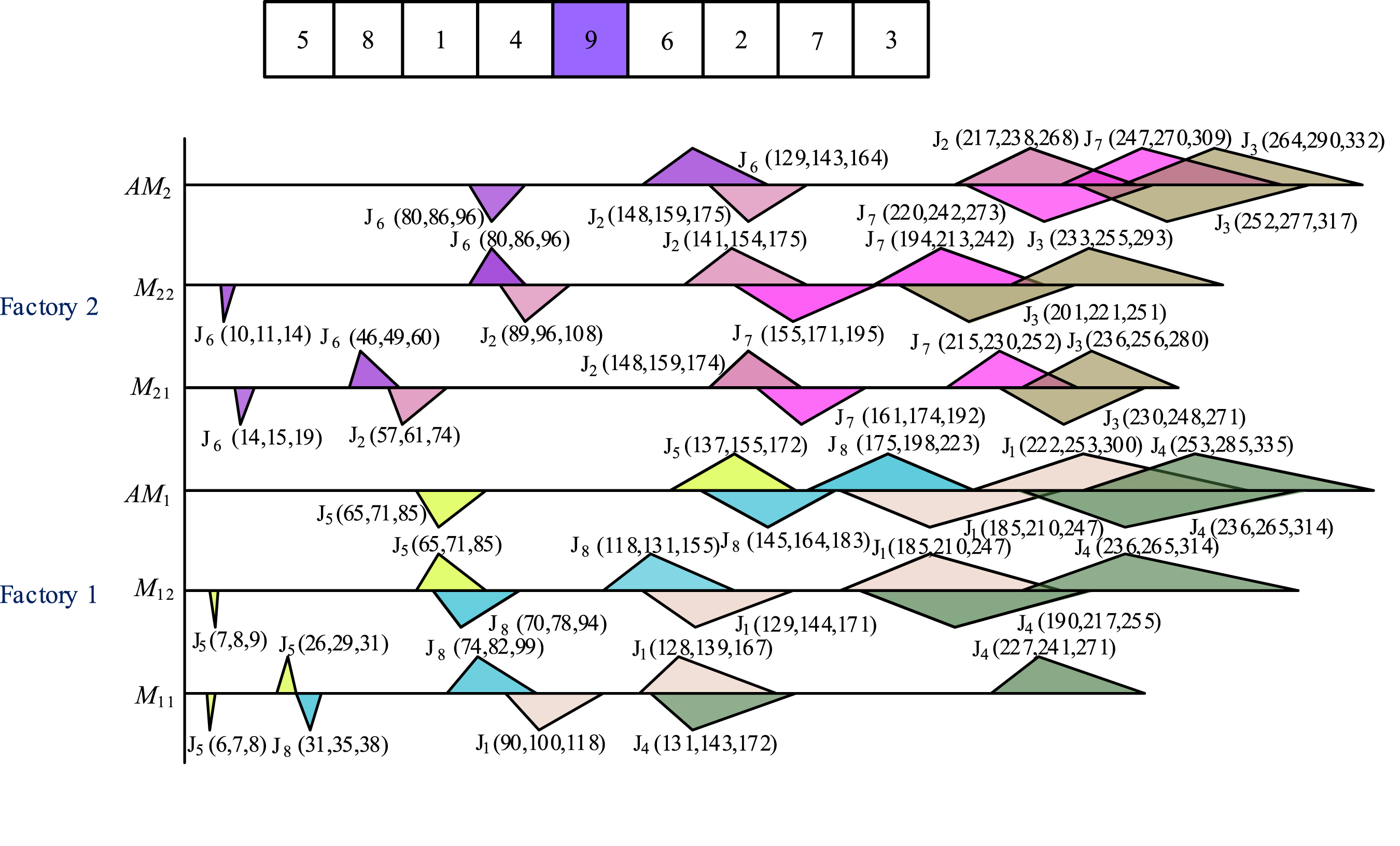
Gantt chart of example.

The population P is initialized by randomly generating N solutions.

After the initial population is constructed, directly sort all solutions of P in a ascending order of fitness f_i, where $f_{i} = {\tilde{C}}_{i, max}$ and ${\tilde{C}}_{i, max}$ indicates fuzzy makespan of solution x_i. Suppose that f₁ ≤ f₂ ≤ ⋯ ≤ f_N, then evenly assign N solutions into s subpopulations according to the following rules sequentially.

If $floor (\frac{k}{s}) = 2 * n$ , allocate s solutions 2 * n * s + 1, 2 * n * s + 2, ⋯ , (2 * n + 1) * s to sub₁, sub₂, ⋯ , sub_s in positive order.

If $floor (\frac{k}{s}) = 2 * n + 1$ , allocate s solutions (2 * n + 1) * s + 1, (2 * n + 1) * s + 2, ⋯ , 2 * (n + 1) * s to sub₁, sub₂, ⋯ , sub_s in reverse order.

where $floor (\frac{k}{s})$ represents the largest integer not greater than $\frac{k}{s}$ , sub_i is the ith subpopulation.

For sub_i, its quality M_i is evaluated by $M_{i} = \frac{\sum_{j \in su b_{i}} F_{j}}{\sum_{k \in P} F_{k}} + \frac{\sum_{j \in su b_{i}} {Num}_{j}^{Iter}}{\sum_{k \in P} {Num}_{k}^{Iter}}$ (9) $F_{j} = 1 - \frac{{\bar{f}}_{j}}{\sum_{j \in P} {\bar{f}}_{j}}$ (10) where F_j is the normalized fitness value of solution x_j, ${\bar{f}}_{j}$ is obtained by $Z_{1} ({\tilde{x}}_{j}) = \frac{{(x_{j})}_{1} + 2 * {(x_{j})}_{2} + {(x_{j})}_{3}}{4}$ , ${Num}_{j}^{Iter}$ indicates the number of improved solutions in generation Iter.

Sort M_i in descending order, suppose that M₁ > ⋯ > M_j > ⋯ > M_s. Calculate average quality $\bar{M}$ and construct employed bee subpopulations and onlooker bee subpopulations based on $\bar{M}$ . If $M_{j} > \bar{M}$ , allocate sub_j (1, 2, ⋯ , m) into employed bee subpopulations EB₁, EB₂, ⋯ , EB_m and put the remaining s - m subpopulations into onlooker bee subpopulations OB₁, OB₂, ⋯, OB_s-m.

5.2 Employed bee phase

Employed bees compete to get the chance of generating new solutions. The detailed search process is described in Algorithm 2, where λ_best is the best solution of EB_i.

In Algorithm 2, both global search(GS) and multiple neighborhood search(NS) are executed on the winner between x and y, so the excellent computing resource in each subpopulation is utilized by the stronger to improve search efficiency. That is, employed bees obtain computing resources and generate new solutions by competing.

Algorithm 2
Employed bee phase

for each solution x ∈ EB_i (1 ≤ i ≤ m) do

2: if m > 1 then

3: stochastically choose y ∈ EB_t (t ≠ i) and the best solution λ_best in EB_i

4: if x is better than y then

5: perform GS (x, λ_best, x, t) on x and λ_best

6: conduct NS (x, x, t) on x

7: else

8: conduct GS (y, λ_best, x, t) on y and λ_best

9: apply NS (x, x, t) to x

10: end if

11: else

12: randomly select y ∈ EB_i (x ≠ y)

13: obtain the winner z by competing between x and y

14: conduct GS (z, λ_best, x, t) and NS (z, z, t) on z

15: end if

16: update Ω_t and Num_x

17: end for

Order-based crossover(OBX) operator is designed for GS. For OBX between x and y, randomly choose g elements from x and delete these picked elements from y. Then generate x_new by filling in the blanks in y with the chosen elements in the order that they appeared in x. g is set to be 8 by experiments. The process of OBX is shown in Fig. 3.

Fig. 3
Order-based crossover

GS (x, y, z, t) is described below. Generate a new solution x_new by performing OBX between x and y, compare it with z. If x_new is better than z, renew the history data set Ω_t with z and update z with x_new; otherwise, renew Ω_t with x_new.

Ω_t is especially designed to record the historical optimization data for sub_t. Its update process is as follows: The initial Ω_t is empty. If z is allowed to update Ω_t, we directly add solution z to Ω_t until |Ω_t| exceeds |Ω_t|_max. To guarantee |Ω_t| is no more than |Ω_t|_max, we calculate the fitness value f_i of all solutions and delete the worst solutions to keep |Ω_t|_max solutions left in Ω_t. |Ω_t|_max = 15 by many experiments.

Three neighborhood structures including exter-factory insert N₁, exter-factory swap N₂ and inter-factory swap N₃ [18] are adopted to implement NS, which are shown in Fig. 4.

Fig. 4
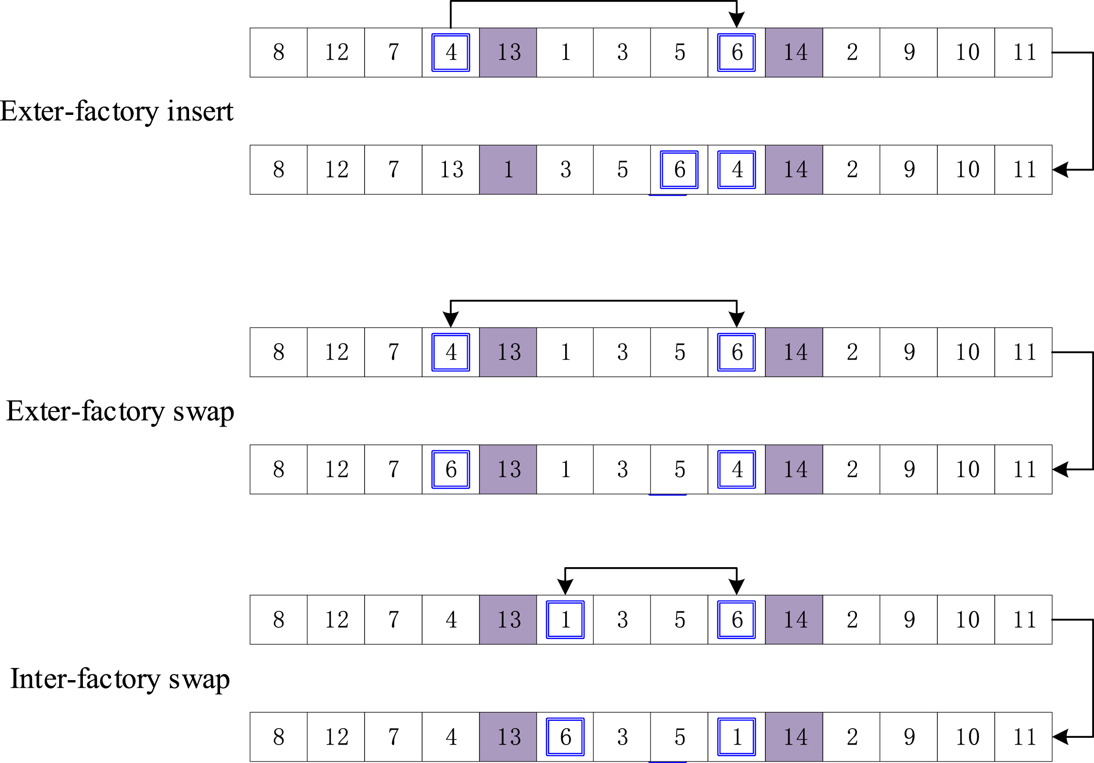
Multiple neighbour structures

NS (x, y, t) is displayed below. For a solution x, set l = 1, w = 1, and repeat the following steps R times: if l = 1, N₁ is performed on x; if l = 2, N₂ is used on x and if l = 3, N₃ is applied. After that, a new solution x_new ∈ N_l (x) is produced. If x_new is better than y, then renew Ω_t with y and substitute y with x_new; else update Ω_t with x_new, l = l + 1 and let l = 1 if l = 4. Where N_l (x) is a set of neighborhood solutions generated by N_l on x and R is an integer.
5.3 Onlooker bee phase

Onlooker bees follow and learn from the elite solutions in employed bee subpopulation. They track the good performance of employed bees through global search and multiple neighborhood search. The detailed search procedure is shown in Algorithm 3, where rand is a rand number in [0,1] and φ is the neighborhood search probability, |φ| = 0.3 and |Φ| = 10 according to lots of experiments.

Algorithm 3
Onlooker bee phase

1: choose several elite solutions from the employed bee subpopulation to construct Φ

2: for t = s - m + 1 to s do

3: for each solution x ∈ OB_t do

4: randomly select a solution y from Φ

5: execute GS (x, y, x, t) between x and y

6: if rand < φ then

7: execute NS (x, x, t) on x

8: end if

9: end for

10: end for

In Algorithm 3, all onlooker bees follow a part of excellent employed bees and conduct the neighborhood search in a small probability to increase the population diversity.
5.4 Scout bee phase

In basic ABC, scout bee phase is used to substitute for a hopeless solution by generating a random one. However, this method is characterized by strong randomness and low efficiency. In this article, the scout bee x is updated as follows: First, select a random employed bee subpopulation EB_k and obtain the best solution y from EB_k, then conduct global search GS (y, z, x, k) on y and a random solution z from Ω_k, and execute neighborhood search NS (x, x, k) on x. After that, the substitution rules are performed to update x and Ω_k. The novel scout bee phase is beneficial to avoid early convergence. The main steps of modified scout bee phase are displayed in Algorithm 4, where trial_i indicates the number of trials for x.

Algorithm 4
Scout bee phase

1: for each solution x ∈ P do

2: if trial_i > Limit then

3: randomly select an employed bee subpopulation EB_k, 1 ≤ k ≤ m

4: choose the best solution y of EB_k and a random solution z in Ω_k

5: perform GS (y, z, x, k) and NS (x, x, k)

6: update x and Ω_k according to the substitution rules

7: end if

8: end for

For sub_t, the poor solutions are exchanged with the ones in Ω_t, which can avoid wasting computing resources. The detailed exchange process is below. First, put all the solutions in Ω_t into sub_t and calculate the fitness value for all, then exclude the worst ones to keep the number of sub_t unchanged. In this way, the population is updated, and the computing resources are fully utilized.

When the above phases are finished, the population is recombined and regrouped, which is the same as the division of the initial population.
5.5 Algorithm description

The detailed procedure of EABC is shown in Algorithm 5.

Algorithm 5
EABC

1: Initialize the population P and parameters

2: Divide P into s subpopulations, construct initial EB and OB

3: while the stopping condition is not met do

4: employed bee phase: compete with other solutions and generate new solutions

5: onlooker bee phase: construct a set of elite employed bees Φ and track the excellent performance in Φ

6: scout bee phase

7: update Ω_t and exchange the worst solutions in sub_t with Ω_t

8: redivide the population P into EB and OB

9: end while

The time complexity of EABC for FDAFSP is O (G_max × N × (n - F + 1) × R), where F is the number of factories, n indicates the number of jobs, G_max represents the maximum number of generations.

There are some features in EABC: (1) A novel subpopulation division method combining the characteristics of the problem is constructed. (2) A competitive search strategy is applied in employed bee phase, and a tracking search strategy is used for onlooker bees to improve search efficiency. (3)The historical optimization data set and a novel scout bee phase are developed. These features can take advantage of computing resources and void premature. As a result, the search efficiency and effectiveness are greatly improved.
6 Numerical results and comparisons

A series of experiments are conducted to verify the performance of EABC for FDAFSP and compiled in Microsoft Visual C++ 2015 and run on 4.0G RAM 2.00GHz CPU PC.

6.1 Test instances and comparative algorithms

Since there are no test instances on FDAFSP, we adopt 50 instances from [17], which are extended by adding fuzzy processing information. TFN ${\tilde{p}}_{ik} = (w_{1} \times p_{ik}, p_{ik}, w_{2} \times p_{ik})$ , where real numbers w₁ ∈ [0.85, 1] and w₂ ∈ [1, 1.3]. TFN ${\tilde{s}}_{ik} = (w_{1} \times s_{ik}, s_{ik}, w_{2} \times s_{ik})$ , ${\tilde{a}}_{i} = (w_{1} \times a_{i}, a_{i}, w_{2} \times a_{i})$ , ${\tilde{u}}_{i} = (w_{1} \times u_{i}, u_{i}, w_{2} \times u_{i})$ . p_ik, s_ik, a_i and u_i are from the original instance [17]. All the above data except w₁ and w₂ are integer.

To verify the performance of EABC, several comparative algorithms are chosen, including ECICA [20], GA-RVNS [17], VNS [17], CMA [18] and DIWO [24].

GA-RVNS and VNS are both used to minimize the weighted sum of mean completion time and makespan of FDAFSP. They can be utilized to solve FDAFSP by setting the mean completion time to zero.

CMA is proposed to solve DAFSP with makespan minimization, which can be directly used to compare with EABC for FDAFSP by simply adding fuzzy information into CMA.

DIWO is developed for DAFSP with total flowtime minimization. By adapting the related objective function, DIWO can be applied to FDAFSP.

ECICA is presented for FDAFSP, in which an adaptive imperialist cooperation between the strongest empire and the weakest empire is performed. Thus, these algorithms are selected to conduct the comparison experiments.

6.2 Parameter settings

In this study, the termination condition is determined by CPU time. We found by experiments that EABC can converge well on all instances when 0.2 × n CPU time reaches; moreover, all selected comparative algorithms also converge fully under this stopping condition. Therefore, we set 0.2 × n as the termination condition for all algorithms.

There are four main parameters in EABC: N, s, Limit, R. Taguchi method is adopted to determine the settings for four parameters. The levels of each parameter are shown in Table 2, and the orthogonal array L₁₆ (4⁴) is given in Table 3.

Table 2
Parameters and their levels

Parameter Factor level

1 2 3 4

N 40 60 80 100

s 3 4 5 6

Limit 4 6 8 10

R 8 10 12 14

Parameter	Factor level
N	40	60	80	100
s	3	4	5	6
Limit	4	6	8	10
R	8	10	12	14

Table 3

The orthogonal array L₁₆ (4⁴)

Trail	Factor				ARV
	N	s	Limit	R
1	1	1	1	1	300.8
2	1	2	2	2	297.3
3	1	3	3	3	300.0
4	1	4	4	4	301.3
5	2	1	2	3	299.5
6	2	2	1	4	303.0
7	2	3	4	1	297.5
8	2	4	3	2	299.0
9	3	1	3	4	300.3
10	3	2	4	3	299.0
11	3	3	1	2	298.0
12	3	4	2	1	297.0
13	4	1	4	2	303.0
14	4	2	3	1	301.3
15	4	3	2	4	298.8
16	4	4	1	3	301.5

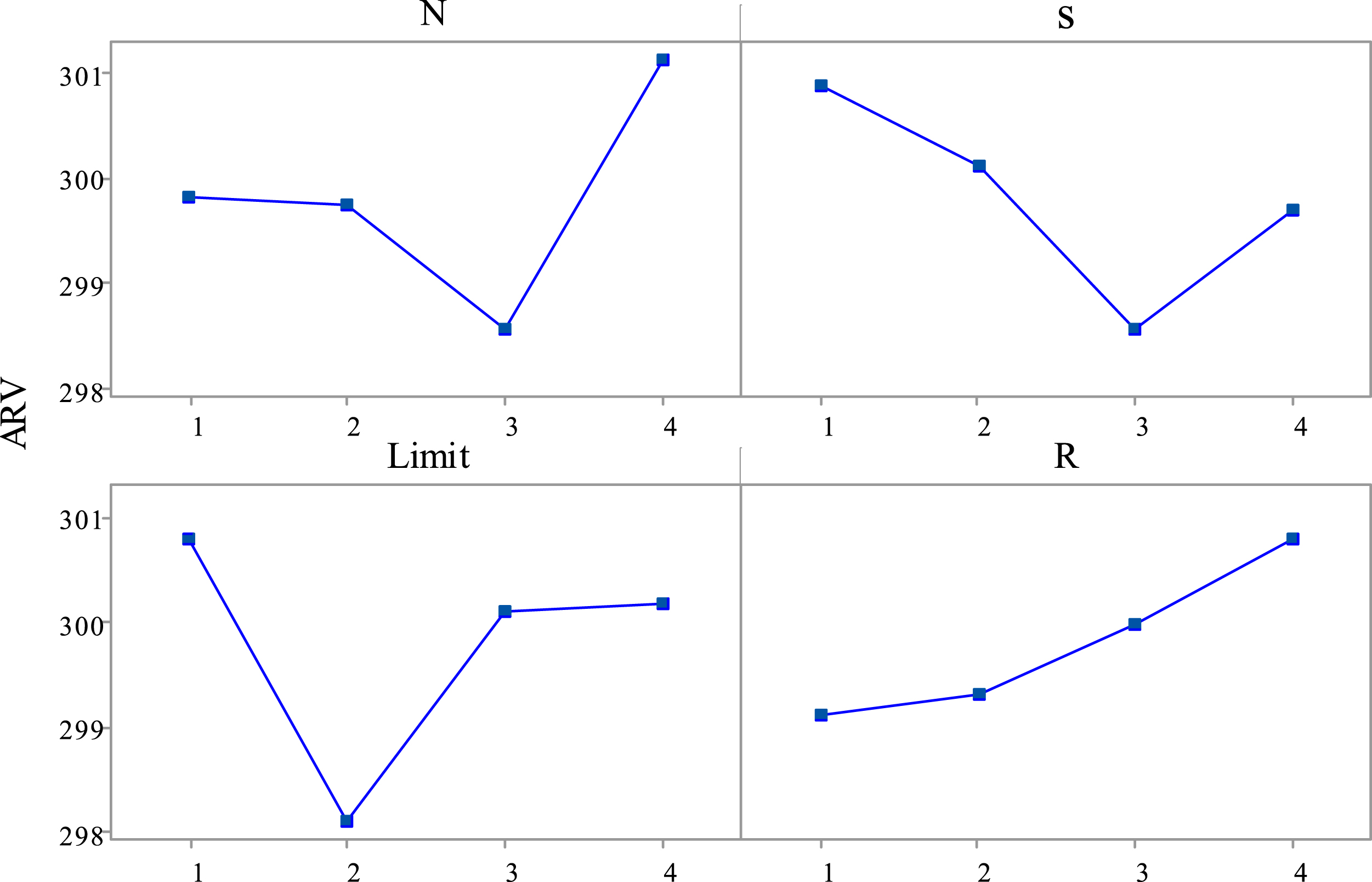
EABC with each combination independently runs 20 times for instance 6 × 20 × 8. The response variable value is denoted as $Z_{1} (C_{max}^{*}) = (t_{1} + 2 t_{2} + t_{3}) / 4$ , where $C_{max}^{*}$ is the elite solution $\tilde{t} = (t_{1}, t_{2}, t_{3})$ obtained in a single run. The average response variable value(ARV) is the average of RV gained over 20 runs. The results of ARV are provided in Fig. 5. Rank of each parameter is shown in Table 4.

Fig. 5

The mean ARV.

Table 4

Response value and rank of each parameter

Level	N	s	Limit	R
1	299.8	300.9	300.8	299.1
2	299.8	300.1	298.1	299.3
3	298.6	298.6	300.1	300.0
4	301.1	299.7	300.2	300.8
Delta	2.6	2.3	2.7	1.7
Rank	2	3	1	4

As shown in Tables 2 –4 and Fig. 5, when the levels of N, s, Limit and R are 3,3,2,1, EABC can produce smaller ARV than EABC with other parameter levels, so we decide that the best settings of parameters in EABC are N = 80, s = 5, Limit = 6 and R = 8.

Meanwhile, it is found by experiments that the original parameter settings of comparative algorithms can result in better performance than other settings, so we directly select the parameters of ECICA, GA-RVNS, VNS, CMA and DIWO from literatures.

6.3 Impact of new strategies of EABC

To test the impact of new strategies of EABC, we construct two variants of EABC, namely EABC1 and EABC2. In EABC1, the subpopulation division process is deleted, so there are no multiple subpopulations. The search process of each phase is identical to that of EABC. The comparison between EABC and EABC1 is used to reveal the impact of the multi-subpopulation division method. In EABC2, the multi-subpopulation division process is preserved, and the search process of each phase is conducted as the general ABC. The contrast between EABC2 and EABC is adopted to show the influence of the novel diversified search process in each phase.

Three algorithms independently run 20 times for each instance. Tables 5 –7 report the comparative results of new strategies on Min, Average and Max, where Min is the minimum solution gained in 20 runs, Max denotes the maximum one obtained in 20 runs, Average indicates the average value of 20 runs.

Table 5
Comparative results of new strategies on Min

Instance Min

EABC EABC1 EABC2

2 × 20 × 4 (611,665,756) (611,665,756) (611,665,756)

2 × 20 × 8 (675,732,841) (675,734,837) (677,727,850)

2 × 50 × 4 (1462,1579,1812) (1469,1572,1819) (1468,1570,1824)

2 × 50 × 8 (1494,1631,1864) (1496,1631,1862) (1492,1632,1864)

2 × 100 × 4 (3018,3294,3778) (3015,3289,3819) (2997,3289,3815)

2 × 100 × 8 (3201,3458,3916) (3180,3458,3937) (3196,3458,3921)

2 × 200 × 4 (5783,6288,7125) (5806,6277,7124) (5792,6277,7138)

2 × 200 × 8 (6075,6634,7661) (6067,6634,7669) (6073,6605,7723)

2 × 500 × 4 (14299,15552,17678) (14285,15553,17692) (14276,15552,17703)

2 × 500 × 8 (14785,16063,18579) (14824,16110,18443) (14799,16116,18456)

3 × 20 × 4 (440,482,552) (438,481,558) (435,476,563)

3 × 20 × 8 (460,509,582) (467,506,587) (466,514,575)

3 × 50 × 4 (941,1033,1170) (943,1031,1176) (948,1031,1173)

3 × 50 × 8 (1050,1150,1328) (1058,1143,1335) (1067,1143,1326)

3 × 100 × 4 (2010,2176,2492) (2003,2194,2463) (1997,2197,2470)

3 × 100 × 8 (2039,2221,2487) (2015,2230,2498) (2020,2213,2558)

3 × 200 × 4 (4013,4343,4991) (3982,4351,5010) (3997,4352,4991)

3 × 200 × 8 (4004,4338,4954) (4001,4341,4956) (3997,4327,4990)

3 × 500 × 4 (9522,10334,11893) (9493,10374,11848) (9519,10347,11895)

3 × 500 × 8 (9648,10489,11917) (9642,10514,11935) (9687,10489,11932)

4 × 20 × 4 (328,358,422) (326,355,415) (337,357,424)

4 × 20 × 8 (429,463,542) (437,467,531) (439,466,531)

4 × 50 × 4 (762,817,957) (756,823,958) (762,825,942)

4 × 50 × 8 (770,849,950) (759,847,966) (767,838,977)

4 × 100 × 4 (1430,1576,1787) (1430,1585,1779) (1428,1572,1806)

4 × 100 × 8 (1526,1653,1876) (1528,1658,1889) (1526,1659,1904)

4 × 200 × 4 (2902,3134,3594) (2883,3148,3592) (2860,3167,3585)

4 × 200 × 8 (2903,3168,3585) (2915,3178,3577) (2857,3179,3620)

4 × 500 × 4 (7286,7925,9050) (7238,7916,9128) (7208,7936,9114)

4 × 500 × 8 (7338,8024,9160) (7342,8035,9150) (7362,8012,9180)

5 × 20 × 4 (295,330,380) (310,326,375) (304,334,372)

5 × 20 × 8 (264,303,358) (290,303,373) (277,306,375)

5 × 50 × 4 (648,687,831) (650,706,800) (643,703,817)

5 × 50 × 8 (627,674,800) (646,692,782) (629,687,798)

5 × 100 × 4 (1236,1350,1522) (1231,1352,1526) (1222,1354,1531)

5 × 100 × 8 (1237,1348,1514) (1232,1343,1547) (1241,1341,1533)

5 × 200 × 4 (2303,2516,2838) (2307,2511,2862) (2305,2515,2842)

5 × 200 × 8 (2394,2574,2977) (2397,2588,3010) (2396,2592,2992)

5 × 500 × 4 (5728,6256,7049) (5718,6245,7099) (5750,6263,7043)

5 × 500 × 8 (5833,6323,7185) (5834,6325,7220) (5828,6334,7256)

6 × 20 × 4 (253,277,328) (256,282,316) (261,279,322)

6 × 20 × 8 (276,299,338) (278,301,326) (273,290,328)

6 × 50 × 4 (495,526,607) (482,541,617) (492,546,610)

6 × 50 × 8 (548,611,722) (577,627,715) (576,624,707)

6 × 100 × 4 (987,1071,1211) (991,1078,1235) (1007,1079,1218)

6 × 100 × 8 (992,1088,1255) (1028,1104,1268) (1014,1097,1278)

6 × 200 × 4 (1897,2087,2386) (1891,2098,2376) (1908,2090,2375)

6 × 200 × 8 (1910,2095,2409) (1978,2113,2425) (1924,2118,2440)

6 × 500 × 4 (4780,5189,5944) (4770,5198,5967) (4765,5231,5911)

6 × 500 × 8 (4860,5268,6081) (4877,5319,6074) (4907,5316,6044)

Instance	Min
2 × 20 × 4	(611,665,756)	(611,665,756)	(611,665,756)
2 × 20 × 8	(675,732,841)	(675,734,837)	(677,727,850)
2 × 50 × 4	(1462,1579,1812)	(1469,1572,1819)	(1468,1570,1824)
2 × 50 × 8	(1494,1631,1864)	(1496,1631,1862)	(1492,1632,1864)
2 × 100 × 4	(3018,3294,3778)	(3015,3289,3819)	(2997,3289,3815)
2 × 100 × 8	(3201,3458,3916)	(3180,3458,3937)	(3196,3458,3921)
2 × 200 × 4	(5783,6288,7125)	(5806,6277,7124)	(5792,6277,7138)
2 × 200 × 8	(6075,6634,7661)	(6067,6634,7669)	(6073,6605,7723)
2 × 500 × 4	(14299,15552,17678)	(14285,15553,17692)	(14276,15552,17703)
2 × 500 × 8	(14785,16063,18579)	(14824,16110,18443)	(14799,16116,18456)
3 × 20 × 4	(440,482,552)	(438,481,558)	(435,476,563)
3 × 20 × 8	(460,509,582)	(467,506,587)	(466,514,575)
3 × 50 × 4	(941,1033,1170)	(943,1031,1176)	(948,1031,1173)
3 × 50 × 8	(1050,1150,1328)	(1058,1143,1335)	(1067,1143,1326)
3 × 100 × 4	(2010,2176,2492)	(2003,2194,2463)	(1997,2197,2470)
3 × 100 × 8	(2039,2221,2487)	(2015,2230,2498)	(2020,2213,2558)
3 × 200 × 4	(4013,4343,4991)	(3982,4351,5010)	(3997,4352,4991)
3 × 200 × 8	(4004,4338,4954)	(4001,4341,4956)	(3997,4327,4990)
3 × 500 × 4	(9522,10334,11893)	(9493,10374,11848)	(9519,10347,11895)
3 × 500 × 8	(9648,10489,11917)	(9642,10514,11935)	(9687,10489,11932)
4 × 20 × 4	(328,358,422)	(326,355,415)	(337,357,424)
4 × 20 × 8	(429,463,542)	(437,467,531)	(439,466,531)
4 × 50 × 4	(762,817,957)	(756,823,958)	(762,825,942)
4 × 50 × 8	(770,849,950)	(759,847,966)	(767,838,977)
4 × 100 × 4	(1430,1576,1787)	(1430,1585,1779)	(1428,1572,1806)
4 × 100 × 8	(1526,1653,1876)	(1528,1658,1889)	(1526,1659,1904)
4 × 200 × 4	(2902,3134,3594)	(2883,3148,3592)	(2860,3167,3585)
4 × 200 × 8	(2903,3168,3585)	(2915,3178,3577)	(2857,3179,3620)
4 × 500 × 4	(7286,7925,9050)	(7238,7916,9128)	(7208,7936,9114)
4 × 500 × 8	(7338,8024,9160)	(7342,8035,9150)	(7362,8012,9180)
5 × 20 × 4	(295,330,380)	(310,326,375)	(304,334,372)
5 × 20 × 8	(264,303,358)	(290,303,373)	(277,306,375)
5 × 50 × 4	(648,687,831)	(650,706,800)	(643,703,817)
5 × 50 × 8	(627,674,800)	(646,692,782)	(629,687,798)
5 × 100 × 4	(1236,1350,1522)	(1231,1352,1526)	(1222,1354,1531)
5 × 100 × 8	(1237,1348,1514)	(1232,1343,1547)	(1241,1341,1533)
5 × 200 × 4	(2303,2516,2838)	(2307,2511,2862)	(2305,2515,2842)
5 × 200 × 8	(2394,2574,2977)	(2397,2588,3010)	(2396,2592,2992)
5 × 500 × 4	(5728,6256,7049)	(5718,6245,7099)	(5750,6263,7043)
5 × 500 × 8	(5833,6323,7185)	(5834,6325,7220)	(5828,6334,7256)
6 × 20 × 4	(253,277,328)	(256,282,316)	(261,279,322)
6 × 20 × 8	(276,299,338)	(278,301,326)	(273,290,328)
6 × 50 × 4	(495,526,607)	(482,541,617)	(492,546,610)
6 × 50 × 8	(548,611,722)	(577,627,715)	(576,624,707)
6 × 100 × 4	(987,1071,1211)	(991,1078,1235)	(1007,1079,1218)
6 × 100 × 8	(992,1088,1255)	(1028,1104,1268)	(1014,1097,1278)
6 × 200 × 4	(1897,2087,2386)	(1891,2098,2376)	(1908,2090,2375)
6 × 200 × 8	(1910,2095,2409)	(1978,2113,2425)	(1924,2118,2440)
6 × 500 × 4	(4780,5189,5944)	(4770,5198,5967)	(4765,5231,5911)
6 × 500 × 8	(4860,5268,6081)	(4877,5319,6074)	(4907,5316,6044)

Table 6

Comparative results of new strategies on Average

Instance	Average
	EABC	EABC1	EABC2
2 × 20 × 4	(608.8,667.6,754.6)	(612.8,668.6,748.4)	(610.4,666.8,755.4)
2 × 20 × 8	(675.1,732.9,839.5)	(678.2,736,830)	(680,734.8,831.4)
2 × 50 × 4	(1458.5,1584.3,1809.6)	(1462.4,1576.8,1816)	(1469.4,1577.8,1809)
2 × 50 × 8	(1488,1631.4,1871.5)	(1485.6,1633.6,1869)	(1494.2,1632.6,1863)
2 × 100 × 4	(3015.1,3298.9,3796.6)	(3019.8,3300.2,3799.4)	(3003.2,3298.8,3811.8)
2 × 100 × 8	(3181.8,3459.4,3932.9)	(3173.2,3460.2,3940.6)	(3174.2,3459,3940.8)
2 × 200 × 4	(5794.1,6268.2,7157.6)	(5776.6,6282.2,7143.8)	(5787.4,6277,7143.2)
2 × 200 × 8	(6083.3,6633.4,7656.8)	(6077,6620.4,7688)	(6081.4,6630.4,7663.8)
2 × 500 × 4	(14280.3,15539.3,17725.7)	(14282.4,15557.4,17689)	(14291.2,15550.8,17691.8)
2 × 500 × 8	(14816.9,16102.7,18478.4)	(14809.4,16113.4,18458.8)	(14795.4,16096.8,18515.4)
3 × 20 × 4	(445.8,483.1,556.3)	(438.2,483.2,568)	(445,480.25,553.5)
3 × 20 × 8	(466.9,514.9,584.5)	(467,514.4,588.6)	(464.4,514.4,584.8)
3 × 50 × 4	(951.3,1031.3,1177.1)	(952.2,1030.4,1186.4)	(956.6,1033.8,1171.4)
3 × 50 × 8	(1063.8,1149.7,1318)	(1066.4,1147.8,1324.8)	(1071.2,1152.2,1310.2)
3 × 100 × 4	(2001,2187.3,2487.3)	(2004,2187.6,2488)	(1997.8,2196.8,2479.6)
3 × 100 × 8	(2037.7,2217.9,2512.1)	(2036.2,2224.6,2520.4)	(2043.6,2224,2533.8)
3 × 200 × 4	(4006.1,4348.6,4988.5)	(3998.6,4354.8,4991.2)	(4003.6,4357.8,4978.8)
3 × 200 × 8	(3989.3,4338.1,4972.6)	(3993.4,4343.6,4961.4)	(3982.8,4339,4982.8)
3 × 500 × 4	(9523.8,10357.5,11870.7)	(9507,10357.4,11891.8)	(9533.4,10372.2,11858.4)
3 × 500 × 8	(9646.1,10485.1,11965.9)	(9663.4,10488.8,11984.4)	(9668.6,10501,11967.2)
4 × 20 × 4	(341.2,364.1,418.2)	(338,362.25,421.75)	(344.2,363.6,418.8)
4 × 20 × 8	(435.3,464.9,537.9)	(439.25,464.5,540)	(434.4,468.4,532.6)
4 × 50 × 4	(762.8,828,941.5)	(764.2,829.6,947)	(764.2,832.2,942.8)
4 × 50 × 8	(773.3,843.7,967.9)	(773.8,844.6,972.6)	(774.8,848.4,966.6)
4 × 100 × 4	(1444.5,1571.8,1789)	(1448.8,1578,1776.4)	(1448.2,1575.2,1792)
4 × 100 × 8	(1518.9,1658.2,1894.2)	(1531.6,1667,1906.2)	(1526.8,1662.8,1906)
4 × 200 × 4	(2875.6,3137.7,3619)	(2888,3146.8,3597.2)	(2879.2,3154.8,3610.4)
4 × 200 × 8	(2899.9,3158.7,3614.6)	(2916.6,3175.4,3602.6)	(2893,3168.2,3622)
4 × 500 × 4	(7280.3,7927.4,9054.1)	(7272.8,7928,9078.2)	(7269,7927,9077.8)
4 × 500 × 8	(7358.2,8019.9,9155)	(7370.4,8031,9155.6)	(7361.6,8020.6,9179.6)
5 × 20 × 4	(304.5,330.3,383.5)	(311.5,332.75,389)	(304.5,335.5,380.75)
5 × 20 × 8	(276.6,305,362)	(297,318.5,374.25)	(287,312.2,371.8)
5 × 50 × 4	(651.8,704.2,801.9)	(649,705.6,814.4)	(641.6,709.6,829.2)
5 × 50 × 8	(632,686.4,790.8)	(645,692.6,797)	(642.6,698.6,800.6)
5 × 100 × 4	(1233.3,1347.3,1535.7)	(1232.8,1349.6,1535.8)	(1237.2,1354.4,1520.2)
5 × 100 × 8	(1238.3,1346.3,1523.6)	(1233.2,1348,1543.6)	(1246,1346.8,1530)
5 × 200 × 4	(2310,2509.1,2849.4)	(2308.6,2522.6,2845.4)	(2311.6,2520.2,2844.6)
5 × 200 × 8	(2388.9,2589.8,2962.6)	(2389.6,2606.8,2999.4)	(2394.8,2603.8,2993.8)
5 × 500 × 4	(5725.4,6230,7107.1)	(5739.8,6232.4,7124)	(5751.8,6244.6,7089.2)
5 × 500 × 8	(5808.1,6319.9,7225.7)	(5828.2,6325.2,7254.6)	(5830.8,6345.8,7247.6)
6 × 20 × 4	(259,281.2,326.2)	(261.8,283.8,319)	(268.8,289.4,327.4)
6 × 20 × 8	(277.4,299.4,337.4)	(289.4,314.8,367)	(288.2,309,351.2)
6 × 50 × 4	(491.8,531.4,608.8)	(490.4,544.2,619)	(493.4,544.6,617.8)
6 × 50 × 8	(564,618.8,708.8)	(576,627.6,725)	(573.75,630.25,721)
6 × 100 × 4	(981,1073.2,1217.6)	(987.2,1083.8,1248.6)	(989.2,1084.6,1238.6)
6 × 100 × 8	(999.8,1089.4,1260)	(1013.2,1107.4,1283.4)	(1020.2,1115,1271.2)
6 × 200 × 4	(1905.8,2073.4,2388.8)	(1912.4,2087,2395.8)	(1923.8,2092.8,2373.6)
6 × 200 × 8	(1922.2,2096.4,2412.8)	(1956.8,2125,2435.8)	(1944,2127.8,2455.2)
6 × 500 × 4	(4768,5193.6,5948.8)	(4799.4,5200.6,5955.8)	(4779.6,5208.2,5962)
6 × 500 × 8	(4879.6,5283.4,6035.6)	(4907,5320.8,6076.6)	(4906.4,5317.2,6053.2)

Table 7

Comparative results of new strategies on Max

Instance	Max
	EABC	EABC1	EABC2
2 × 20 × 4	(600,665,770)	(611,672,745)	(607,669,757)
2 × 20 × 8	(674,731,845)	(677,737,830)	(679,744,815)
2 × 50 × 4	(1458,1587,1800)	(1468,1581,1802)	(1477,1581,1803)
2 × 50 × 8	(1469,1624,1888)	(1476,1629,1891)	(1491,1634,1865)
2 × 100 × 4	(3018,3304,3831)	(3013,3303,3804)	(2999,3305,3812)
2 × 100 × 8	(3107,3459,3948)	(3170,3464,3938)	(3164,3462,3945)
2 × 200 × 4	(5812,6272,7143)	(5768,6277,7164)	(5783,6274,7155)
2 × 200 × 8	(6080,6637,7658)	(6093,6607,7701)	(6079,6639,7649)
2 × 500 × 4	(14369,15520,17684)	(14312,15556,17667)	(14327,15531,17698)
2 × 500 × 8	(14823,16135,18442)	(14812,16109,18474)	(14774,16113,18515)
3 × 20 × 4	(444,488,577)	(459,493,552)	(450,488,543)
3 × 20 × 8	(467,525,601)	(474,525,602)	(465,517,590)
3 × 50 × 4	(962,1032,1180)	(964,1045,1197)	(964,1036,1171)
3 × 50 × 8	(1069,1155,1307)	(1079,1148,1322)	(1073,1157,1300)
3 × 100 × 4	(1997,2183,2512)	(2004,2193,2485)	(2008,2199,2484)
3 × 100 × 8	(2042,2225,2522)	(2068,2226,2510)	(2052,2229,2564)
3 × 200 × 4	(3997,4357,4986)	(3997,4349,5010)	(3988,4369,4977)
3 × 200 × 8	(3974,4349,4970)	(3986,4337,4987)	(3978,4340,4989)
3 × 500 × 4	(9612,10359,11826)	(9529,10353,11907)	(9527,10389,11864)
3 × 500 × 8	(9663,10490,11976)	(9672,10508,11969)	(9702,10508,11958)
4 × 20 × 4	(352,372,421)	(342,371,426)	(346,369,419)
4 × 20 × 8	(435,465,548)	(438,471,533)	(432,467,544)
4 × 50 × 4	(765,838,937)	(771,839,933)	(779,845,929)
4 × 50 × 8	(792,850,944)	(778,843,979)	(779,858,965)
4 × 100 × 4	(1460,1587,1749)	(1459,1586,1752)	(1445,1577,1801)
4 × 100 × 8	(1523,1669,1885)	(1530,1682,1918)	(1533,1671,1894)
4 × 200 × 4	(2881,3140,3619)	(2882,3141,3620)	(2881,3173,3584)
4 × 200 × 8	(2921,3147,3639)	(2943,3182,3589)	(2887,3161,3652)
4 × 500 × 4	(7296,7926,9045)	(7280,7941,9059)	(7285,7943,9040)
4 × 500 × 8	(7378,8021,9149)	(7378,8053,9155)	(7380,8013,9198)
5 × 20 × 4	(321,335,388)	(321,336,393)	(312,345,390)
5 × 20 × 8	(286,309,352)	(310,338,403)	(291,316,375)
5 × 50 × 4	(654,716,787)	(650,702,841)	(647,716,842)
5 × 50 × 8	(634,694,802)	(655,693,805)	(645,700,821)
5 × 100 × 4	(1236,1353,1533)	(1242,1357,1519)	(1256,1352,1512)
5 × 100 × 8	(1243,1347,1529)	(1237,1356,1528)	(1253,1350,1529)
5 × 200 × 4	(2295,2502,2885)	(2303,2529,2844)	(2310,2526,2849)
5 × 200 × 8	(2402,2592,2957)	(2392,2607,3022)	(2400,2621,3018)
5 × 500 × 4	(5729,6209,7152)	(5751,6222,7151)	(5789,6236,7075)
5 × 500 × 8	(5797,6319,7252)	(5813,6337,7250)	(5855,6362,7240)
6 × 20 × 4	(272,286,321)	(272,286,321)	(282,306,344)
6 × 20 × 8	(273,297,353)	(307,337,398)	(311,331,377)
6 × 50 × 4	(490,535,608)	(493,548,638)	(497,547,617)
6 × 50 × 8	(571,626,700)	(587,631,724)	(583,634,724)
6 × 100 × 4	(975,1076,1230)	(988,1087,1256)	(994,1089,1249)
6 × 100 × 8	(993,1093,1283)	(1015,1108,1298)	(1018,1129,1270)
6 × 200 × 4	(1880,2080,2405)	(1906,2082,2444)	(1924,2092,2401)
6 × 200 × 8	(1930,2096,2427)	(1952,2130,2453)	(1974,2140,2440)
6 × 500 × 4	(4779,5188,5951)	(4793,5222,5947)	(4796,5218,5943)
6 × 500 × 8	(4897,5297,6004)	(4936,5338,6073)	(4906,5316,6070)

To make the results statistically convincing, the paired-sample t-test is conducted. The p-value results of t-test are shown in Table 8. The term t-test(A,B) means that a paired t-test is done to judge whether B produces a better sample mean than A. The significance level of 0.05 is assumed, which means that there is a significant difference between A and B in the statistical sense if the p-value is less than 0.05.

Table 8

Results of paired sample t-test

t-test	p-value(Min)	p-value(Average)	p-value(Max)
t-test(EABC,EABC1)	0.000	0.000	0.000
t-test(EABC,EABC2)	0.000	0.000	0.000
t-test(EABC,ECICA)	0.000	0.000	0.000
t-test(EABC,GA-RVNS)	0.000	0.000	0.000
t-test(EABC,VNS)	0.000	0.000	0.000
t-test(EABC,CMA)	0.000	0.000	0.000
t-test(EABC,DIWO)	0.000	0.000	0.000

As stated in Tables 5 –7, EABC provides better results than EABC1 and EABC2 on three metrics. Min of EABC is smaller than that of EABC1 on 42 of 50 instances; Average of EABC is superior to that of EABC1 on 43 of 50 instances; moreover, Max of EABC is better than that of EABC1 on 41 of 50 instances. Compared with EABC2, EABC provides a better Min on 44 of 50 instances and a smaller Average on 44 of 50 instances; moreover, Max of EABC2 is inferior to that of EABC on 40 of 50 instances. The performance differences between EABC and the two variants can also be found in Table 8. Therefore, the new strategies really improve the performance of EABC.

6.4 Results and comparative analysis

For each instance, EABC and five comparative algorithms independently run 20 times. Tables 9 –11 list the results of comparative algorithms on Min, Average and Max. Figures 6 –8 display the box plot of six algorithms on Min, Average and Max, in which Z₁ (Min), Z₁ (Average) and Z₁ (Max) are applied.

Table 9
Result of the comparative algorithms on Min

Instance Min

EABC ECICA GA-RVNS VNS CMA DIWO

2 × 20 × 4 (611,665,756) (611,672,746) (611,672,746) (609,667,755) (607,668,754) (616,662,783)

2 × 20 × 8 (675,732,841) (671,732,845) (675,733,839) (671,732,845) (671,732,845) (681,735,829)

2 × 50 × 4 (1462,1579,1812) (1450,1571,1840) (1459,1590,1793) (1441,1569,1853) (1471,1576,1809) (1463,1584,1802)

2 × 50 × 8 (1494,1631,1864) (1497,1631,1861) (1475,1631,1884) (1511,1631,1847) (1491,1633,1863) (1496,1633,1858)

2 × 100 × 4 (3018,3294,3778) (3008,3294,3788) (3028,3320,3782) (3015,3294,3781) (3010,3298,3801) (3009,3296,3783)

2 × 100 × 8 (3201,3458,3916) (3183,3458,3934) (3184,3460,3929) (3160,3458,3957) (3163,3461,3948) (3186,3459,3929)

2 × 200 × 4 (5783,6288,7125) (5774,6277,7156) (5765,6276,7175) (5749,6283,7169) (5791,6263,7170) (5804,6277,7126)

2 × 200 × 8 (6075,6634,7661) (6053,6634,7683) (6060,6628,7692) (6073,6634,7663) (6056,6650,7650) (6101,6638,7627)

2 × 500 × 4 (14299,15552,17678) (14309,15552,17668) (14319,15553,17662) (14294,15552,17683) (14271,15563,17686) (14300,15554,17673)

2 × 500 × 8 (14785,16063,18579) (14793,16107,18482) (14808,16107,18473) (14880,16106,18397) (14767,16106,18521) (14796,16110,18471)

3 × 20 × 4 (440,482,552) (435,476,563) (447,484,558) (420,476,576) (443,476,561) (441,490,574)

3 × 20 × 8 (460,509,582) (470,503,573) (472,518,593) (454,512,578) (466,509,584) (469,515,600)

3 × 50 × 4 (941,1033,1170) (943,1029,1188) (956,1046,1198) (952,1027,1179) (947,1033,1175) (964,1035,1190)

3 × 50 × 8 (1050,1150,1328) (1046,1145,1342) (1062,1163,1313) (1079,1138,1323) (1060,1144,1333) (1071,1164,1293)

3 × 100 × 4 (2010,2176,2492) (2004,2198,2454) (2024,2207,2503) (1998,2183,2491) (2014,2188,2477) (2010,2199,2483)

3 × 100 × 8 (2039,2221,2487) (2056,2218,2507) (2060,2252,2562) (2035,2213,2513) (2033,2231,2531) (2044,2228,2526)

3 × 200 × 4 (4013,4343,4991) (4034,4345,4966) (4025,4347,5021) (4024,4365,4936) (3975,4343,5034) (4010,4380,4921)

3 × 200 × 8 (4004,4338,4954) (3995,4334,4974) (3990,4341,5019) (3976,4338,4982) (4005,4346,4951) (3992,4345,4958)

3 × 500 × 4 (9522,10334,11893) (9543,10336,11852) (9547,10393,11935) (9507,10341,11903) (9508,10344,11979) (9565,10368,11768)

3 × 500 × 8 (9648,10489,11917) (9669,10490,11918) (9714,10552,12013) (9679,10464,11963) (9671,10522,12069) (9649,10463,11998)

4 × 20 × 4 (328,358,422) (342,362,422) (334,371,425) (326,355,415) (336,361,406) (335,357,410)

4 × 20 × 8 (429,463,542) (435,465,536) (439,463,549) (431,457,550) (438,461,540) (452,486,561)

4 × 50 × 4 (762,817,957) (757,820,963) (779,850,971) (769,831,936) (749,826,965) (777,845,972)

4 × 50 × 8 (770,849,950) (766,844,965) (801,864,986) (785,841,955) (784,840,980) (789,861,979)

4 × 100 × 4 (1430,1576,1787) (1439,1563,1809) (1492,1594,1823) (1451,1569,1784) (1445,1585,1774) (1455,1588,1782)

4 × 100 × 8 (1526,1653,1876) (1515,1656,1916) (1575,1700,1952) (1545,1654,1887) (1548,1671,1915) (1566,1674,1884)

4 × 200 × 4 (2902,3134,3594) (2864,3140,3628) (2939,3200,3679) (2854,3129,3659) (2885,3153,3618) (2894,3156,3634)

4 × 200 × 8 (2903,3168,3585) (2908,3166,3600) (2976,3222,3626) (2892,3169,3606) (2909,3174,3636) (2922,3176,3642)

4 × 500 × 4 (7286,7925,9050) (7273,7911,9100) (7313,7972,9112) (7265,7928,9072) (7271,7949,9039) (7287,7926,9069)

4 × 500 × 8 (7338,8024,9160) (7407,8022,9111) (7408,8067,9162) (7294,8032,9198) (7369,8008,9227) (7327,8031,9163)

5 × 20 × 4 (295,330,380) (296,327,394) (299,342,393) (315,325,379) (301,326,386) (310,326,375)

5 × 20 × 8 (264,303,358) (274,301,367) (292,315,383) (273,307,367) (284,309,358) (273,307,367)

5 × 50 × 4 (648,687,831) (644,703,822) (669,725,847) (643,708,814) (639,701,834) (665,737,798)

5 × 50 × 8 (627,674,800) (645,694,769) (662,720,825) (626,684,799) (656,705,783) (665,719,832)

5 × 100 × 4 (1236,1350,1522) (1232,1348,1537) (1265,1373,1559) (1240,1347,1531) (1215,1353,1554) (1241,1364,1547)

5 × 100 × 8 (1237,1348,1514) (1235,1358,1501) (1290,1366,1573) (1242,1343,1523) (1243,1353,1531) (1238,1346,1567)

5 × 200 × 4 (2303,2516,2838) (2313,2508,2856) (2331,2530,2893) (2306,2517,2839) (2317,2514,2853) (2304,2519,2869)

5 × 200 × 8 (2394,2574,2977) (2389,2593,2984) (2451,2668,3077) (2385,2598,2961) (2436,2633,2970) (2419,2634,3034)

5 × 500 × 4 (5728,6256,7049) (5733,6230,7114) (5820,6296,7196) (5708,6242,7111) (5714,6223,7158) (5733,6229,7129)

5 × 500 × 8 (5833,6323,7185) (5832,6343,7167) (5907,6426,7389) (5825,6324,7217) (5843,6396,7309) (5845,6346,7258)

6 × 20 × 4 (253,277,328) (261,279,322) (273,289,334) (257,286,330) (253,277,328) (253,277,328)

6 × 20 × 8 (276,299,338) (283,295,313) (271,302,354) (275,295,331) (271,297,333) (265,291,340)

6 × 50 × 4 (495,526,607) (489,539,604) (534,576,650) (482,542,616) (496,539,616) (509,556,649)

6 × 50 × 8 (548,611,722) (573,631,700) (614,669,738) (572,625,716) (575,636,715) (592,664,773)

6 × 100 × 4 (987,1071,1211) (972,1065,1241) (1041,1135,1306) (979,1088,1214) (980,1084,1248) (998,1085,1261)

6 × 100 × 8 (992,1088,1255) (1002,1099,1259) (1068,1167,1387) (1021,1095,1280) (1034,1128,1280) (1071,1167,1320)

6 × 200 × 4 (1897,2087,2386) (1931,2078,2368) (1954,2125,2444) (1925,2097,2346) (1897,2090,2410) (1918,2102,2427)

6 × 200 × 8 (1910,2095,2409) (1942,2103,2422) (2087,2226,2555) (1949,2110,2441) (1990,2150,2500) (1994,2161,2438)

6 × 500 × 4 (4780,5189,5944) (4774,5190,5972) (4889,5339,6031) (4763,5189,6006) (4800,5203,5982) (4815,5198,5983)

6 × 500 × 8 (4860,5268,6081) (4900,5290,6077) (5042,5465,6257) (4895,5321,6047) (4990,5352,6159) (4927,5332,6067)

Instance	Min
2 × 20 × 4	(611,665,756)	(611,672,746)	(611,672,746)	(609,667,755)	(607,668,754)	(616,662,783)
2 × 20 × 8	(675,732,841)	(671,732,845)	(675,733,839)	(671,732,845)	(671,732,845)	(681,735,829)
2 × 50 × 4	(1462,1579,1812)	(1450,1571,1840)	(1459,1590,1793)	(1441,1569,1853)	(1471,1576,1809)	(1463,1584,1802)
2 × 50 × 8	(1494,1631,1864)	(1497,1631,1861)	(1475,1631,1884)	(1511,1631,1847)	(1491,1633,1863)	(1496,1633,1858)
2 × 100 × 4	(3018,3294,3778)	(3008,3294,3788)	(3028,3320,3782)	(3015,3294,3781)	(3010,3298,3801)	(3009,3296,3783)
2 × 100 × 8	(3201,3458,3916)	(3183,3458,3934)	(3184,3460,3929)	(3160,3458,3957)	(3163,3461,3948)	(3186,3459,3929)
2 × 200 × 4	(5783,6288,7125)	(5774,6277,7156)	(5765,6276,7175)	(5749,6283,7169)	(5791,6263,7170)	(5804,6277,7126)
2 × 200 × 8	(6075,6634,7661)	(6053,6634,7683)	(6060,6628,7692)	(6073,6634,7663)	(6056,6650,7650)	(6101,6638,7627)
2 × 500 × 4	(14299,15552,17678)	(14309,15552,17668)	(14319,15553,17662)	(14294,15552,17683)	(14271,15563,17686)	(14300,15554,17673)
2 × 500 × 8	(14785,16063,18579)	(14793,16107,18482)	(14808,16107,18473)	(14880,16106,18397)	(14767,16106,18521)	(14796,16110,18471)
3 × 20 × 4	(440,482,552)	(435,476,563)	(447,484,558)	(420,476,576)	(443,476,561)	(441,490,574)
3 × 20 × 8	(460,509,582)	(470,503,573)	(472,518,593)	(454,512,578)	(466,509,584)	(469,515,600)
3 × 50 × 4	(941,1033,1170)	(943,1029,1188)	(956,1046,1198)	(952,1027,1179)	(947,1033,1175)	(964,1035,1190)
3 × 50 × 8	(1050,1150,1328)	(1046,1145,1342)	(1062,1163,1313)	(1079,1138,1323)	(1060,1144,1333)	(1071,1164,1293)
3 × 100 × 4	(2010,2176,2492)	(2004,2198,2454)	(2024,2207,2503)	(1998,2183,2491)	(2014,2188,2477)	(2010,2199,2483)
3 × 100 × 8	(2039,2221,2487)	(2056,2218,2507)	(2060,2252,2562)	(2035,2213,2513)	(2033,2231,2531)	(2044,2228,2526)
3 × 200 × 4	(4013,4343,4991)	(4034,4345,4966)	(4025,4347,5021)	(4024,4365,4936)	(3975,4343,5034)	(4010,4380,4921)
3 × 200 × 8	(4004,4338,4954)	(3995,4334,4974)	(3990,4341,5019)	(3976,4338,4982)	(4005,4346,4951)	(3992,4345,4958)
3 × 500 × 4	(9522,10334,11893)	(9543,10336,11852)	(9547,10393,11935)	(9507,10341,11903)	(9508,10344,11979)	(9565,10368,11768)
3 × 500 × 8	(9648,10489,11917)	(9669,10490,11918)	(9714,10552,12013)	(9679,10464,11963)	(9671,10522,12069)	(9649,10463,11998)
4 × 20 × 4	(328,358,422)	(342,362,422)	(334,371,425)	(326,355,415)	(336,361,406)	(335,357,410)
4 × 20 × 8	(429,463,542)	(435,465,536)	(439,463,549)	(431,457,550)	(438,461,540)	(452,486,561)
4 × 50 × 4	(762,817,957)	(757,820,963)	(779,850,971)	(769,831,936)	(749,826,965)	(777,845,972)
4 × 50 × 8	(770,849,950)	(766,844,965)	(801,864,986)	(785,841,955)	(784,840,980)	(789,861,979)
4 × 100 × 4	(1430,1576,1787)	(1439,1563,1809)	(1492,1594,1823)	(1451,1569,1784)	(1445,1585,1774)	(1455,1588,1782)
4 × 100 × 8	(1526,1653,1876)	(1515,1656,1916)	(1575,1700,1952)	(1545,1654,1887)	(1548,1671,1915)	(1566,1674,1884)
4 × 200 × 4	(2902,3134,3594)	(2864,3140,3628)	(2939,3200,3679)	(2854,3129,3659)	(2885,3153,3618)	(2894,3156,3634)
4 × 200 × 8	(2903,3168,3585)	(2908,3166,3600)	(2976,3222,3626)	(2892,3169,3606)	(2909,3174,3636)	(2922,3176,3642)
4 × 500 × 4	(7286,7925,9050)	(7273,7911,9100)	(7313,7972,9112)	(7265,7928,9072)	(7271,7949,9039)	(7287,7926,9069)
4 × 500 × 8	(7338,8024,9160)	(7407,8022,9111)	(7408,8067,9162)	(7294,8032,9198)	(7369,8008,9227)	(7327,8031,9163)
5 × 20 × 4	(295,330,380)	(296,327,394)	(299,342,393)	(315,325,379)	(301,326,386)	(310,326,375)
5 × 20 × 8	(264,303,358)	(274,301,367)	(292,315,383)	(273,307,367)	(284,309,358)	(273,307,367)
5 × 50 × 4	(648,687,831)	(644,703,822)	(669,725,847)	(643,708,814)	(639,701,834)	(665,737,798)
5 × 50 × 8	(627,674,800)	(645,694,769)	(662,720,825)	(626,684,799)	(656,705,783)	(665,719,832)
5 × 100 × 4	(1236,1350,1522)	(1232,1348,1537)	(1265,1373,1559)	(1240,1347,1531)	(1215,1353,1554)	(1241,1364,1547)
5 × 100 × 8	(1237,1348,1514)	(1235,1358,1501)	(1290,1366,1573)	(1242,1343,1523)	(1243,1353,1531)	(1238,1346,1567)
5 × 200 × 4	(2303,2516,2838)	(2313,2508,2856)	(2331,2530,2893)	(2306,2517,2839)	(2317,2514,2853)	(2304,2519,2869)
5 × 200 × 8	(2394,2574,2977)	(2389,2593,2984)	(2451,2668,3077)	(2385,2598,2961)	(2436,2633,2970)	(2419,2634,3034)
5 × 500 × 4	(5728,6256,7049)	(5733,6230,7114)	(5820,6296,7196)	(5708,6242,7111)	(5714,6223,7158)	(5733,6229,7129)
5 × 500 × 8	(5833,6323,7185)	(5832,6343,7167)	(5907,6426,7389)	(5825,6324,7217)	(5843,6396,7309)	(5845,6346,7258)
6 × 20 × 4	(253,277,328)	(261,279,322)	(273,289,334)	(257,286,330)	(253,277,328)	(253,277,328)
6 × 20 × 8	(276,299,338)	(283,295,313)	(271,302,354)	(275,295,331)	(271,297,333)	(265,291,340)
6 × 50 × 4	(495,526,607)	(489,539,604)	(534,576,650)	(482,542,616)	(496,539,616)	(509,556,649)
6 × 50 × 8	(548,611,722)	(573,631,700)	(614,669,738)	(572,625,716)	(575,636,715)	(592,664,773)
6 × 100 × 4	(987,1071,1211)	(972,1065,1241)	(1041,1135,1306)	(979,1088,1214)	(980,1084,1248)	(998,1085,1261)
6 × 100 × 8	(992,1088,1255)	(1002,1099,1259)	(1068,1167,1387)	(1021,1095,1280)	(1034,1128,1280)	(1071,1167,1320)
6 × 200 × 4	(1897,2087,2386)	(1931,2078,2368)	(1954,2125,2444)	(1925,2097,2346)	(1897,2090,2410)	(1918,2102,2427)
6 × 200 × 8	(1910,2095,2409)	(1942,2103,2422)	(2087,2226,2555)	(1949,2110,2441)	(1990,2150,2500)	(1994,2161,2438)
6 × 500 × 4	(4780,5189,5944)	(4774,5190,5972)	(4889,5339,6031)	(4763,5189,6006)	(4800,5203,5982)	(4815,5198,5983)
6 × 500 × 8	(4860,5268,6081)	(4900,5290,6077)	(5042,5465,6257)	(4895,5321,6047)	(4990,5352,6159)	(4927,5332,6067)

Table 10

Results of the comparative algorithms on Average

Instance	Average
	EABC	ECICA	GA-RVNS	VNS	CMA	DIWO
2 × 20 × 4	(608.8,667.6,754.6)	(605.8,668.8,763.6)	(608.6,668,763.4)	(604.4,665.6,763.4)	(604.4,665.8,762.8)	(616.6,670.4,776.6)
2 × 20 × 8	(675.1,732.9,839.5)	(677.2,733,837)	(673.5,732.7,842.1)	(675.9,733.3,837.8)	(675.3,733.3,838.6)	(676.5,732.5,845.3)
2 × 50 × 4	(1458.5,1584.3,1809.6)	(1460.2,1578,1815.8)	(1464.1,1589.9,1807)	(1453.8,1577.6,1823.5)	(1455.2,1583.3,1810.7)	(1458.4,1587.5,1811.9)
2 × 50 × 8	(1488,1631.4,1871.5)	(1489.4,1632.2,1867)	(1492,1630.9,1877.7)	(1489.9,1631.9,1866.7)	(1488.7,1631.9,1869)	(1491.6,1629.9,1876.4)
2 × 100 × 4	(3015.1,3298.9,3796.6)	(3009.6,3298.4,3805.8)	(3036.1,3317.5,3808.9)	(3010.3,3301.5,3805.2)	(3018.4,3300.9,3799.4)	(3017.1,3298.7,3793.6)
2 × 100 × 8	(3181.8,3459.4,3932.9)	(3173.2,3458.2,3944)	(3182.5,3460.5,3939.4)	(3170.7,3459.8,3944.3)	(3175.4,3461.65,3937.7)	(3174.9,3457.3,3949.1)
2 × 200 × 4	(5794.1,6268.2,7157.6)	(5790.6,6262.4,7170.2)	(5787.2,6282.7,7158.8)	(5789.9,6259.9,7176.8)	(5784.4,6277.5,7151.2)	(5787.5,6275.2,7148.7)
2 × 200 × 8	(6083.3,6633.4,7656.8)	(6077.4,6617,7696.6)	(6083.5,6638,7661.7)	(6082.7,6627.9,7667.2)	(6084.5,6637.4,7650.8)	(6085.7,6628.9,7662.6)
2 × 500 × 4	(14280.3,15539.3,17725.7)	(14299.4,15526,17731.2)	(14283,15555.3,17717.9)	(14295.6,15535,17718.1)	(14268.5,15554.3,17712.4)	(14279.2,15549.4,17706.5)
2 × 500 × 8	(14816.9,16102.7,18478.4)	(14826,16103,18465.4)	(14816.8,16118,18485.2)	(14823.3,16091.4,18488.1)	(14815.3,16122.4,18457.3)	(14813.1,16106.3,18464.8)
3 × 20 × 4	(445.8,483.1,556.3)	(439.6,481.2,556.4)	(449.6,488.55,568.4)	(440.8,481.9,558.4)	(439.3,481.8,560.2)	(463.8,506.5,577.1)
3 × 20 × 8	(466.9,514.9,584.5)	(464.2,510,581.4)	(476.2,524.6,601.8)	(465.1,516.1,590.2)	(468.1,514.1,586.4)	(488.4,537.8,613.9)
3 × 50 × 4	(951.3,1031.3,1177.1)	(949.4,1032.4,1182)	(971.5,105.4,1212.7)	(950.2,1033.3,1180.1)	(953.7,1033.1,1185.4)	(970.1,1051.9,1204.6)
3 × 50 × 8	(1063.8,1149.7,1318)	(1058.4,1149,1323.2)	(1077,1163.9,1322.4)	(1066.9,1146.3,1323.9)	(1063.5,1151,1322.2)	(1077.7,1161.8,1320.3)
3 × 100 × 4	(2001,2187.3,2487.3)	(2004.2,2186,2486)	(2033.8,2220,2533.1)	(1995.7,2192.3,2485.7)	(2001.8,2188.8,2503.6)	(2015.4,2207.6,2508.9)
3 × 100 × 8	(2037.7,2217.9,2512.1)	(2044,2227.4,2517.6)	(2078.3,2262,2569.8)	(2044.9,2224.5,2516.9)	(2052.8,2230.7,2538.9)	(2060.3,2238.7,2542.7)
3 × 200 × 4	(4006.1,4348.6,4988.5)	(4004.8,4353.8,4981.8)	(4019.1,4372.8,5014.6)	(3998.1,4351.3,4993.1)	(4004.6,4363.1,4974)	(4010.8,4356.9,4987.6)
3 × 200 × 8	(3989.3,4338.1,4972.6)	(3989.6,4344.4,4960.8)	(4017.1,4367.2,4997.1)	(3987.1,4340.9,4973.3)	(3998.4,4349.6,4973.5)	(3999.3,4344.1,4971.7)
3 × 500 × 4	(9523.8,10357.5,11870.7)	(9522.2,10363.8,11862.8)	(9574.9,10412.6,11923.4)	(9535.8,10362.9,11867.7)	(9550.2,10382.8,11887.2)	(9516.2,10367.8,11874.5)
3 × 500 × 8	(9646.1,10485.1,11965.9)	(9645.4,10496.4,11968)	(9734.2,10596,12095.8)	(9658.7,10491.7,11976.7	(9703.3,10544.7,12042.4)	(9668.3,10495.6,11979.1)
4 × 20 × 4	(341.2,364.1,418.2)	(345.4,366.4,417)	(348.5,373.5,428)	(344.7,371.1,426)	(339.7,363.5,415.1)	(336.5,363.5,414.4)
4 × 20 × 8	(435.3,464.9,537.9)	(449.6,480.8,554)	(442.5,470.1,543.4)	(434.9,463.4,539.8)	(436.7,464.9,537.9)	(452,486,561)
4 × 50 × 4	(762.8,828,941.5)	(766.2,830.4,949.8)	(791.5,860.9,984.3)	(763.6,836.2,951.5)	(763.8,834.3,947.6)	(789.7,859.5,978.7)
4 × 50 × 8	(773.3,843.7,967.9)	(771.8,846.8,969.6)	(802.6,870.1,1002.4)	(777.1,841.9,970.5)	(778.2,850,975.1)	(799.8,879,1006)
4 × 100 × 4	(1444.5,1571.8,1789)	(1444.8,1576.2,1781)	(1483.8,1611.2,1830.6)	(1446.2,1574.6,1789.7)	(1450.7,1580.2,1786.2)	(1474.7,1599.5,1811.2)
4 × 100 × 8	(1518.9,1658.2,1894.2)	(1525.4,1663,1902.2)	(1580.3,1715.8,1963.3)	(1533.7,1665.8,1898.8)	(1543,1677.4,1914.5)	(1557.1,1691.9,1938.5)
4 × 200 × 4	(2875.6,3137.7,3619)	(2879,3147.6,3612.4)	(2951.5,3223.8,3683)	(2874.4,3147.2,3613.2)	(2889.7,3153.4,3620.9)	(2907.7,3167.2,3632.8)
4 × 200 × 8	(2899.9,3158.7,3614.6)	(2904.2,3165.2,3610.2)	(2976.6,3240,3690)	(2899.7,3165.5,3622.4)	(2916.4,3180,3643.2)	(2928.8,3190.6,3647.7)
4 × 500 × 4	(7280.3,7927.4,9054.1)	(7283.4,7922.2,9081.8)	(7335.5,7996.1,9158.9)	(7296.5,7927.4,9051.1)	(7307,7936.2,9054.8)	(7298.4,7939,9060.5)
4 × 500 × 8	(7358.2,8019.9,9155)	(7372.8,8036.8,9128.2)	(7414.4,8069.5,9202.8)	(7352.5,8026.6,9172.5)	(7407.6,8040.2,9159)	(7388.7,8028.7,9162)
5 × 20 × 4	(304.5,330.3,383.5)	(314.6,341.4,397.4)	(313.3,342.8,397.6)	(308.4,332.3,391.5)	(303.1,329.7,382.4)	(303.8,328.5,381.9)
5 × 20 × 8	(276.6,305,362)	(290.5,315.1,372.2)	(297.6,320.8,376)	(282.8,306.6,362.8)	(283.6,307.4,367.6)	(282.8,306.6,362.8)
5 × 50 × 4	(651.8,704.2,801.9)	(645.6,707,823.8)	(672.3,736.5,846.1)	(646.9,709.6,814.7)	(647.8,709.2,816)	(682.2,741.4,853.6)
5 × 50 × 8	(632,686.4,790.8)	(641.6,696,787.2)	(674,736,840)	(635.6,693.2,794.1)	(651.1,708,803.6)	(677.9,736.6,852.2)
5 × 100 × 4	(1233.3,1347.3,1535.7)	(1237.8,1347.4,1536.4)	(1264.5,1384.9,1579.9)	(1232.5,1352.1,1533.8)	(1232.9,1352.8,1542.3)	(1261.7,1374,1567.6)
5 × 100 × 8	(1238.3,1346.3,1523.6)	(1232.4,1351,1526.8)	(1278.2,1387.5,1589.2)	(1245.6,1346.2,1530.1)	(1243.8,1352.6,1549.2)	(1261.8,1376.1,1573.1)
5 × 200 × 4	(2310,2509.1,2849.4)	(2313,2517.6,2846.8)	(2356.1,2563.3,2921.9)	(2313.1,2521.6,2837.7)	(2315.7,2523.4,2850.7)	(2319.9,2522.5,2882.4)
5 × 200 × 8	(2388.9,2589.8,2962.6)	(2395.8,2594.2,2985.2)	(2474.9,2689.7,3091.4)	(2389.4,2601.6,2988.6)	(2413.9,2631,3023.2)	(2445.2,2655.3,3046.7)
5 × 500 × 4	(5725.4,6230,7107.1)	(5739,6237,7112.2)	(5846.2,6338.4,7244.9)	(5732.5,6243.3,7100.6)	(5739.3,6248.6,7129.4)	(5746.8,6248.4,7135.7)
5 × 500 × 8	(5808.1,6319.9,7225.7)	(5828.8,6334.4,7241)	(5939.7,6474.3,7406.4)	(5817.7,6334.7,7249)	(5877.4,6399.6,7331.1)	(5864,6368.5,7280.8)
6 × 20 × 4	(259,281.2,326.2)	(261.8,285.8,332)	(272.6,294.2,336.6)	(265.6,291.8,339.2)	(258.4,279,327.2)	(256.8,282,325.4)
6 × 20 × 8	(277.4,299.4,337.4)	(284.8,308.4,352.2)	(285.2,307.6,356.8)	(278.6,300.2,341.4)	(274.8,295.6,336)	(276,293.2,331.4)
6 × 50 × 4	(491.8,531.4,608.8)	(491.2,539,616.4)	(534.6,578.6,662.6)	(495.2,540.2,615.8)	(489.8,541,625.2)	(520.6,574.4,658.4)
6 × 50 × 8	(564,618.8,708.8)	(577.6,626.6,716.6)	(613.6,673.2,767.8)	(571.6,625.4,722.6)	(573.8,636,734)	(627,693,794.2)
6 × 100 × 4	(981,1073.2,1217.6)	(984.2,1080.8,1236.4)	(1047.8,1138.2,1313.6)	(988.8,1086.8,1231)	(998.6,1086.6,1235)	(1022,1118.4,1268)
6 × 100 × 8	(999.8,1089.4,1260)	(1023.6,1107,1259.8)	(1079.8,1183.2,1374)	(1028.2,1106.8,1284.8)	(1027.8,1130.2,1290.8)	(1082,1177.6,1344.6)
6 × 200 × 4	(1905.8,2073.4,2388.8)	(1919,2084,2377.8)	(1985.8,2163.2,2481.8)	(1924.6,2085.8,2384)	(1909.6,2090.2,2405.6)	(1956.2,2119,2444.8)
6 × 200 × 8	(1922.2,2096.4,2412.8)	(1951.6,2117.6,2439)	(2079,2245.8,2565.6)	(1959.4,2117.6,2442.8)	(1984.4,2156.6,2496.6)	(2006.6,2199.4,2504)
6 × 500 × 4	(4768,5193.6,5948.8)	(4775.8,5209.4,5945.8)	(4895.8,5328.8,6082.2)	(4795.8,5198.2,5972)	(4803.6,5215.6,5969.8)	(4808,5221.8,5973)
6 × 500 × 8	(4879.6,5283.4,6035.6)	(4896.4,5313,6059.4)	(5053.6,5491.2,6284.6)	(4916.8,5321.6,6058)	(4980.6,5386,6146.2)	(4936.8,5357,6105.6)

Table 11

Results of the comparative algorithms on Max

Instance	Max
	EABC	ECICA	GA-RVNS	VNS	CMA	DIWO
2 × 20 × 4	(600,665,770)	(608,671,767)	(614,678,742)	(600,665,770)	(605,662,773)	(621,675,776)
2 × 20 × 8	(674,731,845)	(677,727,850)	(671,731,850)	(672,733,843)	(676,738,829)	(681,739,847)
2 × 50 × 4	(1458,1587,1800)	(1466,1582,1802)	(1468,1592,1820)	(1461,1578,1823)	(1463,1580,1812)	(1469,1597,1813)
2 × 50 × 8	(1469,1624,1888)	(1490,1632,1870)	(1482,1636,1901)	(1486,1632,1874)	(1477,1630,1889)	(1491,1633,1893)
2 × 100 × 4	(3018,3304,3831)	(3012,3307,3797)	(3035,3324,3821)	(3019,3297,3844)	(3010,3307,3807)	(3004,3300,3834)
2 × 100 × 8	(3107,3459,3948)	(3168,3459,3950)	(3206,3462,3922)	(3169,3452,3970)	(3179,3459,3945)	(3187,3464,3938)
2 × 200 × 4	(5812,6272,7143)	(5765,6277,7167)	(5778,6290,7181)	(5787,6261,7186)	(5788,6287,7131)	(5779,6284,7153)
2 × 200 × 8	(6080,6637,7658)	(6082,6624,7682)	(6069,6632,7712)	(6106,6617,7672)	(6117,6630,7639)	(6078,6632,7688)
2 × 500 × 4	(14369,15520,17684)	(14264,15501,17819)	(14263,15579,17710)	(14321,15556,17656)	(14281,15565,17684)	(14297,15535,17741)
2 × 500 × 8	(14823,16135,18442)	(14878,16080,18467)	(14804,16121,18551)	(14806,16109,18480)	(14792,16130,18481)	(14822,16123,18441)
3 × 20 × 4	(444,488,577)	(432,484,568)	(455,492,575)	(448,485,569)	(447,486,557)	(474,514,605)
3 × 20 × 8	(467,525,601)	(465,520,581)	(479,537,595)	(464,531,600)	(467,516,600)	(498,547,649)
3 × 50 × 4	(962,1032,1180)	(950,1042,1174)	(987,1054,1235)	(950,1036,1192)	(954,1033,1194)	(983,1065,1238)
3 × 50 × 8	(1069,1155,1307)	(1070,1149,1313)	(1095,1163,1325)	(1053,1154,1336)	(1059,1153,1329)	(1091,1177,1334)
3 × 100 × 4	(1997,2183,2512)	(2008,2176,2512)	(2041,2221,2577)	(1999,2189,2505)	(1989,2177,2549)	(2031,2224,2532)
3 × 100 × 8	(2042,2225,2522)	(2046,2230,2536)	(2078,2277,2589)	(2065,2234,2518)	(2073,2236,2533)	(2101,2263,2571)
3 × 200 × 4	(3997,4357,4986)	(4018,4345,4998)	(4040,4390,4999)	(3985,4356,5001)	(3976,4362,5012)	(4061,4385,4930)
3 × 200 × 8	(3974,4349,4970)	(4002,4346,4947)	(4043,4372,5059)	(3047,4348,5010)	(3997,4365,4986)	(4000,4354,4999)
3 × 500 × 4	(9612,10359,11826)	(9537,10377,11858)	(9576,10435,11958)	(9586,10376,11865)	(9621,10387,11845)	(9558,10381,11887)
3 × 500 × 8	(9663,10490,11976)	(9649,10508,11965)	(9742,10644,12221)	(9647,10512,12008)	(9710,10551,12086)	(9731,10534,11964)
4 × 20 × 4	(352,372,421)	(341,368,428)	(358,377,438)	(405,434,491)	(344,367,418)	(331,363,433)
4 × 20 × 8	(435,465,548)	(512,543,618)	(457,471,540)	(441,462,544)	(440,459,552)	(452,486,561)
4 × 50 × 4	(765,838,937)	(775,837,936)	(797,868,991)	(770,840,965)	(766,832,958)	(798,871,988)
4 × 50 × 8	(792,850,944)	(774,843,984)	(822,875,1005)	(782,840,985)	(789,857,960)	(838,903,1028)
4 × 100 × 4	(1460,1587,1749)	(1434,1579,1792)	(1491,1621,1857)	(1438,1582,1799)	(1452,1587,1795)	(1474,1612,1841)
4 × 100 × 8	(1523,1669,1885)	(1530,1667,1905)	(1569,1723,1988)	(1536,1669,1928)	(1556,1683,1907)	(1578,1729,1966)
4 × 200 × 4	(2881,3140,3619)	(2892,3150,3620)	(2960,3251,3665)	(2898,3163,3580)	(2890,3159,3621)	(2926,3179,3635)
4 × 200 × 8	(2921,3147,3639)	(2896,3163,3631)	(2997,3267,3733)	(2914,3182,3607)	(2917,3186,3662)	(2968,3191,3680)
4 × 500 × 4	(7296,7926,9045)	(7263,7932,9088)	(7341,8028,9188)	(7316,7949,9006)	(7288,7945,9068)	(7308,7939,9080)
4 × 500 × 8	(7378,8021,9149)	(7325,8021,9231)	(7434,8106,9196)	(7368,8022,9182)	(7449,8050,9136)	(7404,8071,9153)
5 × 20 × 4	(321,335,388)	(334,362,416)	(324,347,398)	(321,348,424)	(308,334,375)	(304,329,388)
5 × 20 × 8	(286,309,352)	(320,343,408)	(302,326,377)	(286,311,356)	(290,308,366)	(286,311,356)
5 × 50 × 4	(654,716,787)	(647,714,837)	(685,743,845)	(648,719,807)	(644,707,834)	(685,749,894)
5 × 50 × 8	(634,694,802)	(645,702,810)	(685,753,837)	(641,700,797)	(650,725,790)	(686,750,872)
5 × 100 × 4	(1236,1353,1533)	(1241,1352,1529)	(1280,1392,1591)	(1247,1355,1523)	(1232,1359,1539)	(1273,1388,1577)
5 × 100 × 8	(1243,1347,1529)	(1259,1348,1515)	(1292,1394,1599)	(1260,1353,1526)	(1242,1345,1576)	(1269,1399,1616)
5 × 200 × 4	(2295,2502,2885)	(2310,2532,2828)	(2386,2589,2924)	(2325,2530,2836)	(2305,2506,2902)	(2326,2509,2931)
5 × 200 × 8	(2402,2592,2957)	(2410,2590,2987)	(2479,2712,3110)	(2383,2618,3005)	(2412,2636,3036)	(2470,2688,3092)
5 × 500 × 4	(5729,6209,7152)	(5743,6247,7122)	(5920,6362,7291)	(5764,6274,7050)	(5743,6268,7103)	(5772,6266,7149)
5 × 500 × 8	(5797,6319,7252)	(5813,6333,7247)	(5979,6513,7453)	(5823,6358,7252)	(5878,6408,7367)	(5907,6404,7292)
6 × 20 × 4	(272,286,321)	(272,299,333)	(279,295,338)	(290,315,365)	(266,280,328)	(257,285,331)
6 × 20 × 8	(273,297,353)	(305,336,391)	(284,311,373)	(295,318,354)	(278,301,326)	(269,296,337)
6 × 50 × 4	(490,535,608)	(494,543,624)	(538,586,678)	(505,547,620)	(494,548,618)	(528,589,665)
6 × 50 × 8	(571,626,700)	(588,630,720)	(619,679,788)	(567,630,726)	(569,637,750)	(637,711,810)
6 × 100 × 4	(975,1076,1230)	(1001,1086,1233)	(1056,1143,1326)	(998,1086,1251)	(1014,1088,1224)	(1035,1133,1276)
6 × 100 × 8	(993,1093,1283)	(1050,1121,1259)	(1080,1188,1389)	(1033,1108,1302)	(1024,1116,1333)	(1088,1197,1376)
6 × 200 × 4	(1880,2080,2405)	(1936,2093,2354)	(2001,2198,2482)	(1961,2076,2393)	(1911,2107,2383)	(1970,2131,2512)
6 × 200 × 8	(1930,2096,2427)	(1960,2135,2454)	(2086,2259,2602)	(1995,2130,2413)	(1966,2157,2525)	(2060,2237,2546)
6 × 500 × 4	(4779,5188,5951)	(4776,5208,5960)	(4908,5351,6143)	(4811,5212,5953)	(4756,5230,6001)	(4806,5222,6009)
6 × 500 × 8	(4897,5297,6004)	(4910,5329,6053)	(5101,5493,6296)	(4927,5333,6059)	(4985,5395,6169)	(4984,5371,6158)

Fig. 6

Box plot of all algorithms on Min.

Fig. 7

Box plot of all algorithms on Average.

Fig. 8

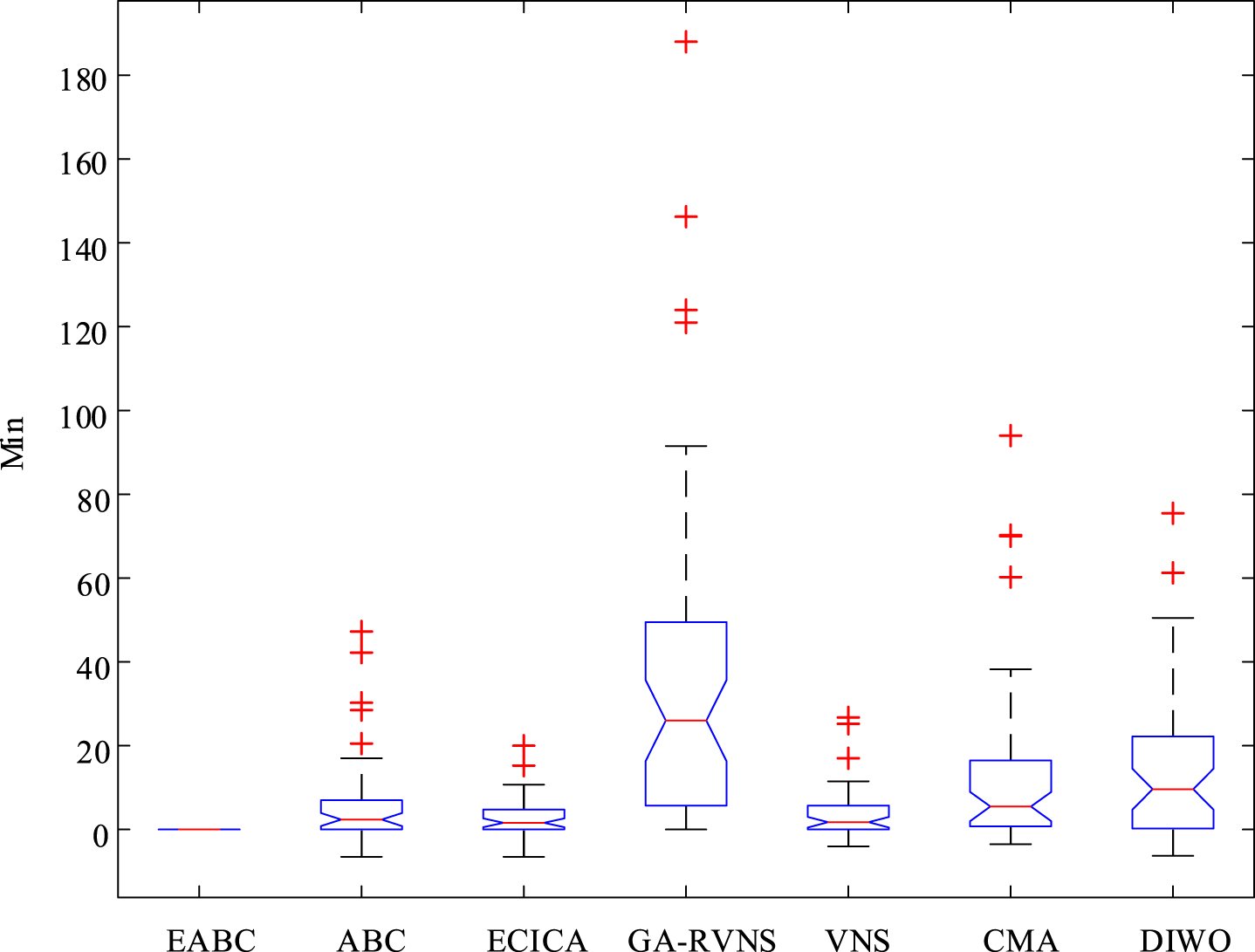
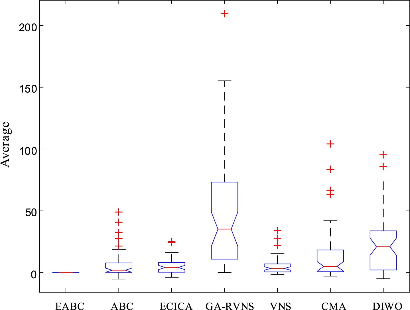
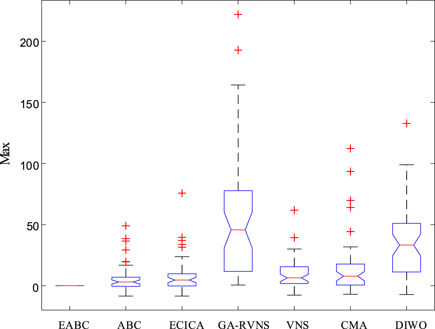
Box plot of all algorithms on Max

As stated in Tables 9 –11, EABC generates better results than the comparative algorithms on Min, Average and Max. Min of EABC is less or identical than that of ECICA, GA-RVNS, VNS, CMA and DIWO on 44, 50, 44, 48 and 46 instances, Average of EABC exceeds that of ECICA, GA-RVNS, VNS, CMA and DIWO on 40, 50, 41, 43 and 41 instances, and smaller Max is possessed than that of ECICA, GA-RVNS, VNS, CMA and DIWO on 37, 50, 45, 40 and 44 instances. That’s to say, EABC performs better than the comparative algorithms on over 74% instances. Meanwhile, it is found from Table 8 that there are significant differences between EABC and its comparative algorithms. This conclusion can also be drawn from Figs. 6 –8. Thus, EABC outperforms the comparative algorithms on metrics.

The above results and comparative analysis reveal the superior performance of EABC on FDAFSP. The excellent performance mainly depends on the usage of a novel subpopulation division method, diversified search strategies implemented in different search phases, and the adoption of a historical optimization data set. These features can effectively improve search efficiency and make a balance between global search and local search. Thus, EABC exhibits excellent capabilities in solving FDAFSP.

7 Conclusions

AFSP in a single factory has been well investigated, but the fuzzy AFSP in multi-factories is seldom studied. In this study, a novel algorithm called EABC is put forward to minimize the fuzzy makespan in FDAFSP with DPm → 1. In EABC, an adaptive subpopulation division method depending on the features of the problem is proposed; a competitive employed bee phase and a novel onlooker bee phase are designed based on the diversified combinations of global search and neighborhood search operators. The historical data set and a novel scout bee phase are also utilized. The effective performance of EABC in solving FDAFSP is verified by a series of comparative experiments.

FDAFSP widely exists in modern manufacturing environments. The research of EABC on FDAFSP also reveals some management implications: the selection of the optimal scheduling scheme will guide the managers to make the smartest production decision and achieve the highest production efficiency. However, there are still some limitations in this research. For example, this paper mainly focuses on the design of the optimization method rather than the improvements of the problem model; moreover, some practical constraints and multi-objective optimization problems are not considered in this study, which are more realistic and challenging. Accordingly, the extension of this problem will be our future research topics, such as multi-constraint, multi-objective, energy-related distributed assembly flow shop scheduling problems. Meanwhile, some new strategies can be adopted to improve search quality and efficiency in shop scheduling, such as the dynamic combination of decision makers’ preferences and the reasonable coordination of pre-event, in-event and post-event decisions.

Footnotes

Acknowledgment

This work is supported by the National Natural Science Foundation of China (62176147).

References

Lee

C.Y.

, Cheng

T.C.E.

and Lin

B.M.T.

, Minimizing the makespan inthe 3-machine assembly-type flow shop scheduling problem, Management Science 39 (1993), 616–625.

Potts

C.N.

, Sevast’janov

S.V.

, Strusevich

V.A.

and VanWassenhove

L.N.

, The two-stage assembly scheduling problem: complexityand approximation, Operations Research 43(2) (1995), 346–355.

Yokoyama

, Scheduling for two-stage production system with setupand assembly operations, Computers and Operations Research 31(12) (2004), 2063–2078.

Fattahi

, Hosseini

S.M.H.

and Jolai

, A mathematical model and extension algorithm for assembly flexible flow shop scheduling problem, International Journal of Advanced Mnufacturing Technology 65(5–8) (2013), 787–802.

Framinan

J.M.

, Perez-Gonzalez

and Fernandez-Viagas

, Deterministic assembly scheduling problems: A review and classification of concurrent-type scheduling models and solution procedures, European Journal of Operational Research 273(2) (2019), 401–417.

Komaki

G.M.

, Teymourian

and Kayvanfar

, Minimising makespan inthe two-stage assembly hybrid flow shop scheduling using artificial immune systems, International Journal of Production Research 54(4) (2016), 963–983.

Allahverdi

and Al-Anzi

F.S.

, Evolutionary heuristics and analgorithm for the two-stage assembly scheduling problem to minimize makespan with setup times, International Journal of Production Research 44(22) (2006), 4713–4735.

C.C.

, Chen

J.Y.

, Lin

W.C.

and Lai

, A two-stage three-machineassembly flow shop scheduling with learning consideration tominimize the flowtime by six hybrids of particle swarm optimization, Swarm and Evolutionary Computation 41 (2018), 97–110.

Shokrollahpour

, Zandieh

and Dorri

, A novel imperialist competitive algorithm for bi-criteria scheduling of the assembly flowshop problem, International Journal of Production Research 49(11) (2011), 3087–3103.

10.

Kazemi

, Mazdeh

M.M.

and Rostami

, The two stage assembly flow-shop scheduling problem with batching and delivery, Engineering Applications of Artificial Intelligence 63(2017), 98–107.

11.

Mozdgir

, Ghomi

S.M.T.F.

, Jolai

and Navaei

, Threemeta-heuristics to solve the no-wait two-stage assembly flow-shop scheduling problem, Scientia Iranica 20(6) (2013), 2275–2283.

12.

Jung

, Woo

Y.B.

and Kim

B.S.

, Two-stage assembly scheduling problem for processing products with dynamic component-sizes and asetup time, Computers and Industrial Engineering 104(2017), 98–113.

13.

Basir

S.A.

, Mazdeh

M.M.

and Namakshenas

, Bi-level genetical gorithms for a two-stage assembly flow-shop scheduling with batch delivery system, Computers and Industrial Engineering 126 (2018), 217–231.

14.

Komaki

G.M.

, Teymourian

, Kayvanfar

and Booyavi

, Improved discrete cuckoo optimization algorithm for the three-stage assembly flowshop scheduling problem, Computers and Industrial Engineering 105 (2017), 158–173.

15.

Azzouz

, Pan

P.A.

, Hsu

P.H.

, Lin

W.C.

, Liu

S.C.

, Ben

S.L.

and Wu

C.C.

, A two-stage three-machine assembly scheduling problem with atruncation position-based learning effect, Soft Computing 24(14) (2020), 10515–10533.

16.

Komaki

G.M.

, Sheikh

and Malakooti

, Flow shop scheduling problems with assembly operations: a review and new trends, International Journal of Production Research 57(10) (2019), 2926–2955.

17.

Xiong

F.L.

and Xing

K.Y.

, Meta-heuristics for the distributed two-stage assembly scheduling problem with bi-criteria of makespan and mean completion time, International Journal of Production Research 52(9) (2014), 2743–2766.

18.

Deng

, Wang

S.Y.

and Zheng

X.L.

, A competitive memetic algorithm for the distributed two-stage assembly flow-shop scheduling problem, International Journal of Production Research 54(12) (2016), 3561–3577.

19.

Lei

D.M.

, Su

and Li

, Cooperated teaching-learning-based optimisation for distributed two-stage assembly flow shop scheduling, International Journal of Production Research 59(23) (2021), 7232–7245.

20.

, Su

and Lei

D.M.

, A novel imperialist competitive algorithm for fuzzy distributed assembly flow shop scheduling, Journal of Intelligent and Fuzzy Systems 40(3) (2021), 4545–4561.

21.

Hatami

, Ruiz

and Andres-Romano

, The distributed assembly permutation flowshop scheduling problem, International Journalof Production Research 51(17) (2021), 5292–5308.

22.

Wang

S.Y.

annd Wang

, An estimation of distribution algorithm-based memetic algorithm for the distributed assembly permutation flow-shop scheduling problem, IEEE Transactions onSystems, Man and Cybernetics: Systems 46(1) (2016), 139–149.

23.

Lin

, Wang

Z.J.

and Li

X.D.

, A backtracking search hyper-heuristicfor the distributed assembly flow-shop scheduling problem, Swarm and Evolutionary Computation 36 (2017), 124–135.

24.

Sang

H.Y.

, Pan

Q.K.

, Li

J.Q.

, Wang

, Han

Y.Y.

, Gao

K.Z.

and Duan

, Effective invasive weed optimization algorithms for distributed assembly permutation flowshop problem with total flowtime criterion, Swarm and Evolutionary Computation 44 (2019), 64–93.

25.

Huang

Y.Y.

, Pan

Q.K.

, Huang

J.P.

, Suganthan

P.N.

and Gao

, An improved iterated greedy algorithm for the distributed assembly permutation flowshop scheduling problem, Computers and Industrial Engineering 152 (2021), 107021.

26.

Zhao

F.Q.

, Di

S.L.

, Wang

, Xu

T.P.

, Zhu

N.N.

and Jonrinaldi. , Aself-learning hyper-heuristic for the distributed assembly blocking flow shop scheduling problem with total flowtime criterion, Engineering Applications of Artificial Intelligence 116(2022), 105418.

27.

Wang

J.J.

and Wang

, A cooperative memetic algorithm with feedbackfor the energy-aware distributed flow-shops with flexible assembly scheduling, Computers and Industrial Engineering 168(2022), 108126.

28.

Zhang

Z.Q.

, Qian

, Hu

, Jin

H.P.

and Wang

, Amatrix-cube-based estimation of distribution algorithm for thedistributed assembly permutation flow-shop scheduling problem, Swarm and Evoultionary Computation 60 (2021), 100785.

29.

Pan

Q.K.

, Gao

, Li

X.Y.

and Jose

F.M.

, Effective constructive heuristics and meta-heuristics for the distributed assembly permutation flowshop scheduling problem, Applied Soft Computing 81 (2019), 105492.

30.

Zadeh

L.A.

, Fuzzy set, Information and Control 8(3) (1965), 338–353.

31.

J.Q.

and Pan

Q.K.

, Chemical-reaction optimization for solving fuzzy job-shop scheduling problem with flexible maintenance activities, International Journal of Production Economics 145(1) (2013), 4–17.

32.

Wang

, Zhou

, Xu

and Liu

, A hybrid artificial bee colony algorithm for the fuzzy flexible job-shop scheduling problem, International Journal of Production Research 51(12) (2013), 3593–3608.

33.

Lei

D.M.

and Guo

X.P.

, Swarm-based neighbourhood search algorithm for fuzzy flexible job shop scheduling, International Journal of Production Research 50(6) (2012), 1639–1649.

34.

Liu

G.S.

, Zhou

and Yang

H.D.

, Minimizing energy consumption and tardiness penalty for fuzzy flow shop scheduling with state-dependent setup time, Journal of Cleaner Production 147 (2017), 470–484.

35.

Lin

, Backtracking search based hyper-heuristic for the flexible job-shop scheduling problem with fuzzy processing time, Engineering Applications of Artificial Intelligence 77(2019), 186–196.

36.

Cai

J.C.

, Zhou

and Lei

D.M.

, Fuzzy distributed two-stage hybrid flow shop scheduling problem with setup time: collaborative variable search, Journal of Intelligent and Fuzzy Systems 38(3) (2020), 3189–3199.

37.

Zheng

, Wang

and Wang

J.J.

, A cooperative coevolution algorithm for multi-objective fuzzy distributed hybrid flow shop, Knowledge-Based Systems 194 (2020), 105536.

38.

Huang

C.E.

and Shi

F.G.

, On the fuzzy dimensions of fuzzy vector spaces, Iranian Journal of Fuzzy Systems 9(4) (2012), 141–150.

39.

Shi

F.G.

and Huang

C.E.

, Fuzzy bases and the fuzzy dimension of fuzzy vector spaces, Mathematical Communications 15(2) (2010), 303–310.

40.

Wang

, Zhu

H.S.

, Wilamowska-Korsak

, Bi

Z.M.

and Li

, Determination of Weights for Multi objective Decision Making or Machine Learning, IEEE Systems Journal 8(1) (2014), 63–72.

41.

Fan

, Li

W.J.

, Cai

X.Y.

, Li

, Wei

C.M.

, Zhang

Q.F.

, Deb

and Goodman.

, Push and pull search for solving constrained multi-objective optimization problems, Swarm and evolutionary computation 44 (2019), 665–679.

42.

Karaboga

and Basturk

, A powerful and efficient algorithm for numerical function optimization: Artificial bee colony (ABC) algorithm, Journal of Global Optimization 39(3) (2007), 459–471.

43.

Karaboga

and Basturk

, On the performance of artificial beecolony (ABC) algorithm, Applied Soft Computing 8(1) (2008), 687–697.

44.

Zuo

Y.D.

, Fan

, Zou

T.R.

and Wang

, A novel multi-population artificial bee colony algorithm for energy-efficient hybrid flowshop scheduling problem, Symmetry-Basel 13(12) (2022), 2421.

45.

Aslan

, Badem

and Karaboga

, Improved quick artificial beecolony (iqABC) algorithm for global optimization, Soft Computing 23(24) (2019), 13161–13182.

46.

Karaboga

and Akay

, A modified artificial bee colony (ABC) algorithm for constrained optimization problems, Applied Soft Computing 11(3) (2011), 3021–3031.

47.

Cui

and Gu

X.S.

, An improved discrete artificial bee colony algorithm to minimize the makespan on hybrid flow shop problems, Neurocomputing 148 (2015), 248–259.

48.

Pan

Q.K.

, Wang

, Li

J.Q.

and Duan

J.H.

, A novel discrete artificial bee colony algorithm for the hybrid flowshop scheduling problem with makespan minimisation, Omega-International Journalof Management Science 45 (2014), 42–56.

49.

J.Q.

, Pan

Q.K.

and Duan

P.Y.

, An improved artificial bee colony algorithm for solving hybrid flexible flowshop with dynamic operation skipping, IEEE Transactions on Cybernetics 46(2016), 1311–1324.

50.

Lin

, Xu

J.Y.

, Baia

D.Y.

, Chung

I.H.

, Liu

S.C.

and Wu

C.C.

, Artificial bee colony algorithms for the order scheduling with release dates, Soft Computing 23(18) (2019), 8677–8688.

51.

Meng

and Pan

Q.K.

, A distributed heterogeneous permutation flowshop scheduling problem with lot-streaming and carryover sequence-dependent setup time, Swarm and Evolutioonary Computation 60 (2021), 100804.

52.

Lei

D.M.

, Yuan

and Cai

J.C.

, An improved artificial bee colony for multi-objective distributed unrelated parallel machine scheduling, International Journal of Production Research 59(17) (2021), 5259–5271.

53.

H.R.

, Li

X.Y.

and Liang

, A discrete artificial bee colony algorithm for the distributed heterogeneous no-wait flowshop scheduling problem, Applied soft computing 100 (2021), 106946.

Minimizing fuzzy makespan in a distributed assembly flow shop by using an efficient artificial bee colony algorithm

Abstract

Keywords

1 Introduction

2 Operations on fuzzy processing time

5.1 Representation and initialization

6.1 Test instances and comparative algorithms

6.2 Parameter settings

Table 2 Parameters and their levels Parameter Factor level 1 2 3 4 N 40 60 80 100 s 3 4 5 6 Limit 4 6 8 10 R 8 10 12 14

Footnotes

Acknowledgment

References

Table 2
Parameters and their levels

Parameter Factor level

1 2 3 4

N 40 60 80 100

s 3 4 5 6

Limit 4 6 8 10

R 8 10 12 14