A two-stage convolution network algorithm for predicting traffic speed based on multi-feature attention mechanisms

Abstract

In recent years, it has been shown that deep learning methods have excellent performance in establishing spatio-temporal correlations for traffic speed prediction. However, due to the complexity of deep learning models, most of them use only short-term historical data in the time dimension, which limits their effectiveness in handling long-term information. We propose a new model, the Multi-feature Two-stage Attention Convolution Network (MTA-CN), to address this issue. The MTA-CN intercepts longer single-feature historical data, converts them into shorter multi-feature data with multiple time period features, and uses the most recent past point as the main feature. Furthermore, two-stage attention mechanisms are introduced to capture the importance of different time period features and time steps, and a Temporal Graph Convolutional Network (T-GCN) is used instead of traditional recurrent neural networks. Experimental results on both the Los Angeles Expressway (Los-loop) and Shen-zhen Luohu District Taxi (Sz-taxi) datasets demonstrate that the proposed model outperforms several baseline models in terms of prediction accuracy.

Keywords

Traffic speed prediction attentional mechanisms temporal dependence spatial dependence graph convolutional network

1 Introduction

With the development of technology, the increase in vehicle ownership per capita inevitably leads to many transportation problems, for example, congestion on transportation networks is a long-standing, hot topic [1–5], and these problems can have some impact on people’s livelihood and social economy [6–8]. In order to solve these traffic problems, it is particularly important to develop intelligent transportation systems [9], which have become the future direction of transportation systems. Traffic speed prediction is an extremely important part of the intelligent transportation system. By accurately predicting the traffic flow, we can effectively analyze the road conditions and avoid the possible future risks in time. It can not only help traffic managers to dispatch and control the traffic system in a timely manner, but also improve the operation efficiency of the traffic network by planning appropriate travel routes in advance for people who travel. However, due to the complex spatial correlation and temporal correlation of traffic data, it has been a challenging task for traffic speed prediction to make suitable models to improve the accuracy of prediction by adequately considering both factors.

In the spatial dimension, traffic data exhibits spatial dependency [10]. The traffic flow of a certain road section is greatly related to the topology of the traffic system of the entire city, the traffic flow between multiple road sections affects each other, and the correlation between different road sections affects the traffic status of the road. While some researchers use Convolutional Neural Networks (CNN) for spatial modeling, it is only applicable to Euclidean spatial structures and cannot be applied to complex topological models like traffic roads. In the time dimension, the traffic data also changes dynamically over time, with the current traffic flow being influenced by the previous or earlier traffic flow. Therefore, accurate traffic speed prediction requires us to pay attention not only to the influence of correlations between time series in different spaces but also to fully consider the long-term temporal patterns.

After observing sufficiently long time series, we found that the computational complexity of the model usually increases with the length of the time series, and deep learning models do not easily scale to long historical time series as the length of the time series increases. Cho et al. [11] pointed out that the performance of the model decreases as the sequence length increases. Most deep learning models typically use shorter historical data to make predictions, such as the past hour, but traffic flow at earlier moments is also closely related to the current traffic flow. For example, people go to work during the morning peak period and leave work during the evening peak period, and the traffic flow during the evening peak period depends largely on the traffic flow during the morning peak period. It is impossible to learn these time patterns from long-term information by selecting only short historical data. The prediction of traffic data requires the observation of long-term data, but for models, long-term data can lead to a loss of accuracy. This contradictory issue requires the model to address the conflict between the lack of long-term data and the decrease in accuracy caused by long-term data in traffic prediction.

To address this problem, Guo et al. [12] intercepted three time series segments along the time axis, representing the most recent, daily, and weekly features, as in Fig. 1. In this way, the model can use shorter historical data while taking into account the long-term information of the time series. However, the intercept positions of these three time series segments are artificially set, and the daily feature with the greatest causal relationship with T_p may not be T_d but T_d1, and the weekly feature with the greatest causal relationship may not be T_w but T_w1. Existing models often manually segment time series data, such as dividing them into days, weeks, or distinguishing between holiday and non-holiday periods. However, in some cases, important features may not be captured by such segmentations, and significant temporal patterns need to be discovered by the model rather than determined by human intuition. How can the model adaptively capture the most important features rather than by artificially selecting specific time series? For this problem we propose a new model Multi-feature Two-stage Attention Convolution Network (MTA-CN). It imports a continuous period of long-term historical data, represents the long-term historical time series fragmentarily into multiple time period features, and learns the temporal correlation of these fragments through an attention mechanism. By using this approach, the model can adaptively capture significant temporal patterns instead of relying on manual segmentation, thereby enabling it to learn temporal patterns from long-term historical data.

Fig. 1

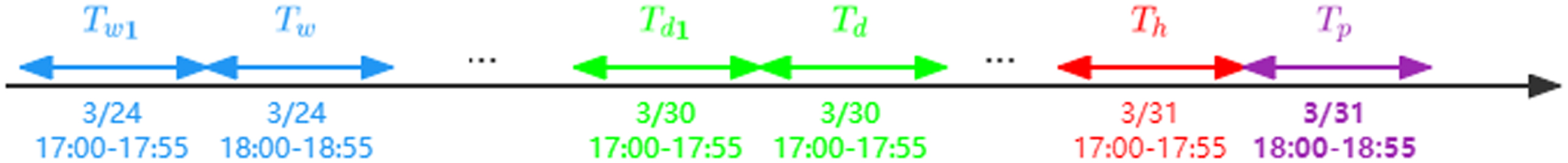
Input of Time Series Segments (Suppose the time step is set to one hour, T_w1, T_w, T_d1, T_d, T_h, T_p are equal in length).

The main contributions of this paper are summarized in the following:

Our model is built by inputting long-term historical data and dividing it into multiple time periods equally, taking the most recent time period as the main feature and the rest as time period features. The model can fully take into account the causality in the time dimension and does not degrade the prediction accuracy due to the long time step.

The model uses a two-stage attention to learn temporal correlation, where time period attention to extract the importance of different time period features, adaptive extraction of relevant driving sequences for each time period features, and temporal attention to select relevant encoder hidden states in the time step.

In the spatial dimension, we use the Graph Convolutional Neural Network (GCN) for extracting spatial features of traffic data, which can extract non-Euclidean spatial structures. The data passes through the GCN and enters the Gated Recurrent Unit (GRU), which is then combined with the attention mechanism as the encoder and decoder of the model.

The rest of the paper is organized as follows. In Section 2, we survey several works related to the traffic speed prediction. In Section 3, we define the model notations and derive the formulations used in the present model. In Section 4, we present a two-stage convolution network algorithm based on multi-feature attention mechanisms. Our experimental results will be conducted in Section 5, and the data analysis will also be presented. Finally, we summarize the conclusions and future research directions of this paper in Section 6.

2 Related works

2.1 Statistical method model

Statistical method models used for traffic speed prediction include the Historical Average model (HA) [13], which has a simple algorithm and can solve the traffic speed prediction problem at different times to some extent. But this model can only be used for static prediction and cannot overcome the influence of disturbing factors. The Autoregressive Integrated Moving Average model (ARIMA) [14] regards the prediction subject as a random time series, converts the non-stationary sequence into a stationary sequence, and then uses a mathematical model to approximate the description of the random sequence. The Vector Autoregressive model (VAR) [15] can better reflect the fluctuation of traffic flow in real time and reduce the uncertainty in the prediction process as much as possible, but it needs to estimate too many parameters. Although these above models can capture the temporal correlation in traffic data, they cannot describe the spatial correlation in road traffic network.

2.2 Machine learning

While the statistical method models have a simple and easy-to-calculate algorithm, they can only be applied to a static model. However, traffic data is often nonlinear and uncertain, and there are random events such as traffic accidents that these models cannot account for. In contrast, traditional machine learning models only need enough data to learn these regularities. Among them, the K-Nearest Neighbor model is one of the most commonly used non-parametric regression models. It can filter historical data and find the nearest neighbors that match the current real-time observation data based on relevant elements from historical data. The function of support vector regression (SVR) is to collect some parameters of the previous period at a certain time as input and output the traffic of the corresponding period. Then it selects the kernel function to train the support vector machine to predict the next stage of data. There are also some classic models such as Bayesian Network (BN) [17] and Kalman Filtering (KF) [18]. However, these models are still unable to describe the spatial correlation of road network topology.

2.3 Deep learning

Compared with machine learning models, deep learning can achieve higher prediction accuracy as the amount of data increases [19]. In the time dimension, because the back propagation neural network has a very good effect in fitting nonlinear data, some researchers use it in traffic speed prediction, but the back propagation neural network also has many shortcomings, such as gradient disappearance and gradient explosion. Some variants of Recurrent Neural Networks (RNN) such as Long Short-Term Memory (LSTM) [20], Sequence to Sequence (Seq2Seq) [21] help to solve this problem. These networks are suitable for many time series prediction problems such as stock price prediction [22], traffic speed prediction [23], and they can overcome the error decay problem of back-propagation to capture long-term dependencies in time series.

Liu et al. [24] proposed an end-to-end deep learning architecture that uses convolution and LSTM combined into a Conv-LSTM module and a bidirectional LSTM to extract the periodic characteristics of traffic flow. Zhang et al. [25] proposed a multi-task learning framework (MDL) for predicting the flow of nodes and edges respectively, which models the correlation between the two types of flows through the regularization of the loss function, which strengthens the prediction for each type of flow. Chen et al. [26] used three deep residual neural networks to simulate the trend properties of time, cycle and traffic flow and proposed a prediction algorithm DeepTFP, which can optimize the parameters of the time series prediction model.

In the spatial dimension, the model Conv-LSTM proposed by Liu et al. [24] uses convolution operations to capture the spatial correlation of the road network. Ranjan et al. [27] proposed a symmetrical U-shaped structure called PredNet, which has CNN blocks at the input and output ends. The performance of this model is stable. Compared with Conv-LSTM, it has higher accuracy and faster training speed. Cheng et al. [28] proposed an end-to-end framework DeepTransport, which uses CNN and RNN and attention mechanism, and the model is used to capture complex relationships in the spatio-temporal domain. Wang et al. [29] used Gaussian regularized residual learning and proposed a new convolutional neural network, which is a Gaussian noise residual network. Chai et al. [30] proposed a new multi-graph convolutional neural network to capture the spatial relationship between different sites, and each graph is learned by a CNN individually. The above methods essentially use CNN to extract the spatial features of traditional Euclidean space, but the traffic road network itself is a complex topology, and CNN cannot be applied to this irregular non-Euclidean space.

ethispage2pt

In recent years, with the development of graph neural networks, some researchers have found that it is very suitable for traffic speed prediction problems, because it can capture the non-Euclidean spatial structure of road networks. Li et al. [31] proposed a new model, Diffused Convolutional Recurrent Neural Network (DCRNN), which captures spatial correlation through bidirectional random walks on the graph. Zhao et al. [32] used GCN [33] to extract non-Euclidean space, in this model, GCN is used as a feature extractor before inputting GRU. Yu et al. [34] also used graph convolutional neural networks to extract spatial features. In addition, the attention mechanism [35] is also used to extract spatio-temporal correlations in traffic speed prediction. Zheng et al. [36, 37] used the attention mechanism to extract the spatio-temporal correlation of the traffic road network, and Abdelraouf et al. [38] combined the attention mechanism with the encoder-decoder architecture.

Some models also incorporate other types of temporal periodicity in addition to recent time series. Guo et al. [12] considered two new time patterns in their model, namely, daily cycle and weekly cycle. Shao et al. [39] considered long-term historical data, while Lu et al. [40] used time-aware convolutional contextual blocks to enhance the network’s ability to capture more distinguishable temporal features. Pan et al. [41] divided time into two categories, weekdays and weekends.

3 Problem formulation

3.1 Problem definition

In this paper, the traffic road network is defined as an undirected graph G = (V, E, A), where the notation V = (v₁, v₂, …, v_N) represents a node in the road network corresponding to N sensors, the notation E denotes a set of edges representing node connections, while the notation A ∈ R^N×N represents the adjacency matrix of the network.Note that the notation A ∈ R^N×N is used to represent the connection between nodes. If nodes i and j are connected, and the graph is a weighted graph, then A_i,j is the proximity between two nodes, otherwise it is 1. If the nodes i and j are not connected to each other, A_i,j = 0.

Table 1
Summary of notation

Notation Description

T Time step

N Number of nodes

C Number of features

τ Time of prediction

h_t Encoder hidden layer state

n Number of time period features

Subscript main Main feature

Subscript s Time period feature

$χ_{main}^{r}$ The main feature sequence at time r

X Time period feature sequence after feature sampling

a Encoder hidden layers

$e_{t}^{k}$ The attention weight of the kth time period feature

$\bar{x}$ The current state of the encoder

B Decoder hidden layers

$i_{t}^{k}$ Attention weights at the kth time step

c_t Context vector

y^* The current state of the decoder

d_t Decoder hidden layer state

$\hat{y}$ Final predicted value

Notation	Description
T	Time step
N	Number of nodes
C	Number of features
τ	Time of prediction
h_t	Encoder hidden layer state
n	Number of time period features
Subscript main	Main feature
Subscript s	Time period feature
$χ_{main}^{r}$	The main feature sequence at time r
X	Time period feature sequence after feature sampling
a	Encoder hidden layers
$e_{t}^{k}$	The attention weight of the kth time period feature
$\bar{x}$	The current state of the encoder
B	Decoder hidden layers
$i_{t}^{k}$	Attention weights at the kth time step
c_t	Context vector
y^*	The current state of the decoder
d_t	Decoder hidden layer state
$\hat{y}$	Final predicted value

The symbol X ∈ R^N×C represents the characteristic matrix of the road network, traffic speed is regarded as the attribute of the node, and the symbol C represents the number of attribute features of the node. Let X_t denote the observation of the road network at time step t. Our problem is defined as: Given the historical time step T observations of all nodes χ = (X_t+1, X_t+2, …, X_t+T) ∈ R^T×N×C, predict the traffic situation of all nodes in the time series of the next time step τ. We use (X_t+T+1, …, X_t+T+τ) ∈ R^T×N×C to represent the future length as τ The traffic situation of the time series, as shown in Equation (1): $[X_{t + T + 1}, \dots, X_{t + T + τ}] = f (X_{t + 1}, X_{t + 2}, \dots, X_{t + T}),$ (1) where f represents the nonlinear function to be learned.

3.2 GCN

When dealing with spatial structures in the past, the road network is usually divided into several grids equally, and then the CNN is used to extract the local spatial structure features, but this method only uses the grid structure with the structural norms. This method is not suitable for the non-Euclidean spatial structure of the traffic road network. Therefore, the GCN, which can extend the convolution operation to any graph structure, has received extensive attention in recent years, and it can be better applied to the extraction of spatial structure features of traffic road networks. GCN ingeniously designed a method to extract features from graph data. It uses spectral graph theory to realize convolution operations on topological graphs. Specifically, it maps graph signals to the frequency domain and then performs convolution operations. As shown in Fig. 2, the red node represents the target node to be aggregated, and the blue node represents the node adjacent to the red node. GCN can extract the topological relationship between the target node and the adjacent nodes. We define L = D - A as the Laplacian matrix of a graph, where D represents the degree matrix and A is the adjacency matrix of the graph. The Laplacian matrix reflects the cumulative gain generated when the current node disturbs the surrounding nodes, which can describe the degree of change in the graph. The formula of GCN is as follows:

Fig. 2

Red nodes represent target nodes. (a) The blue part represents the aggregated other node information. (b) Obtain the topological relationship of the target node and the adjacent blue nodes.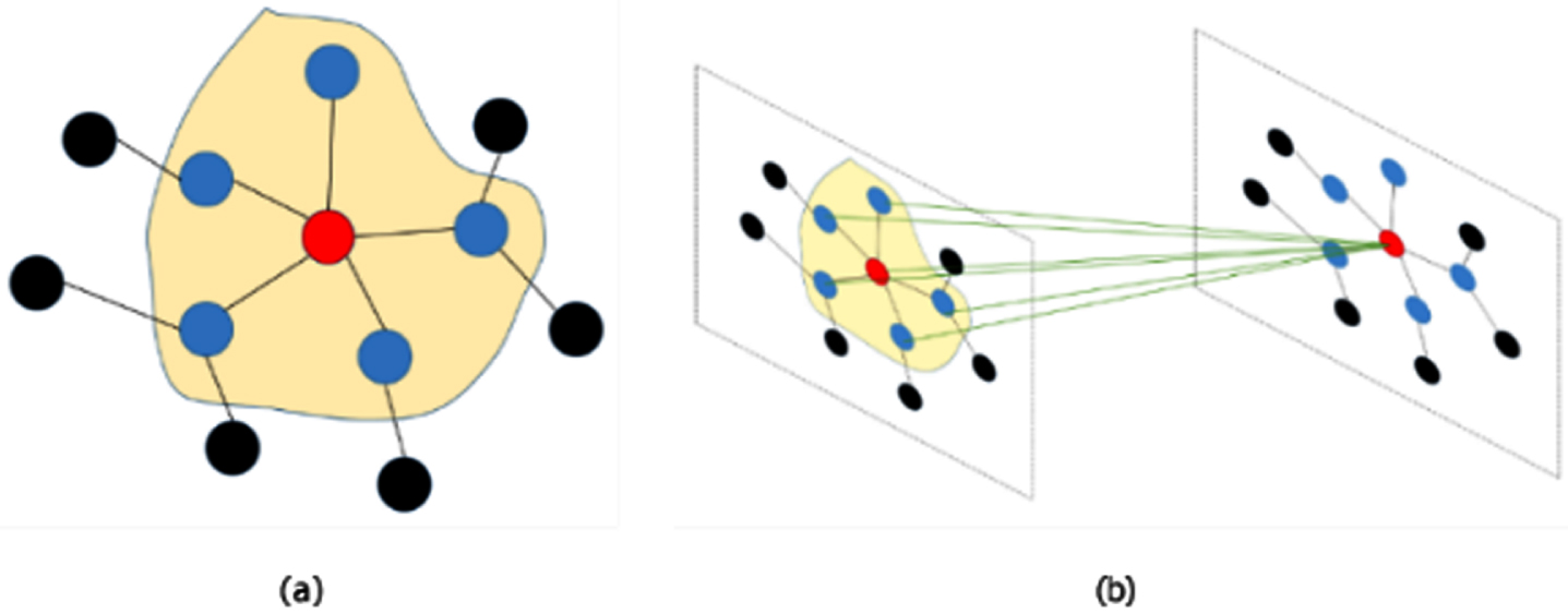

\hat{A} = {\tilde{D}}^{- \frac{1}{2}} \tilde{A} {\tilde{D}}^{- \frac{1}{2}},

(2)

GCN (X, A) = σ (\hat{ARelu} (\hat{AX} W_{0}) W_{1}),

(3) where the notation X represents the feature matrix, the notation A represents the adjacency matrix.

\tilde{A} = A + E

represents the adjacency matrix with self-connection added, and the notation E represents the identity matrix.

\tilde{D} = Σ_{j} {\tilde{A}}_{ij}

is the degree matrix. W₀ ∈ R^C×H, W₁ ∈ R^H×T are learnable parameters, which respectively represent the weight matrix from the input to the hidden layer and the weight matrix from the hidden layer to the output layer. The notation C represents the number of features, and the symbol H represents the number of hidden layers.

3.3 GRU

The most widely used to capture temporal correlation is RNN. However, because of the problem of gradient explosion and gradient disappearance, more and more researches use RNN’s variant LSTM to capture temporal correlation. Another variant, GRU is similar to the internal principles of LSTM. Compared to the LSTM, which has many parameters and is difficult to train, the GRU has a simpler structure with fewer parameters, is easy to implement, and achieves the same results with less time cost and computational power [42], so we choose the GRU to capture temporal correlation. Its structure is shown in Fig. 3, where r_t represents the reset gate, which determines how to combine the new input information with the previous memory. 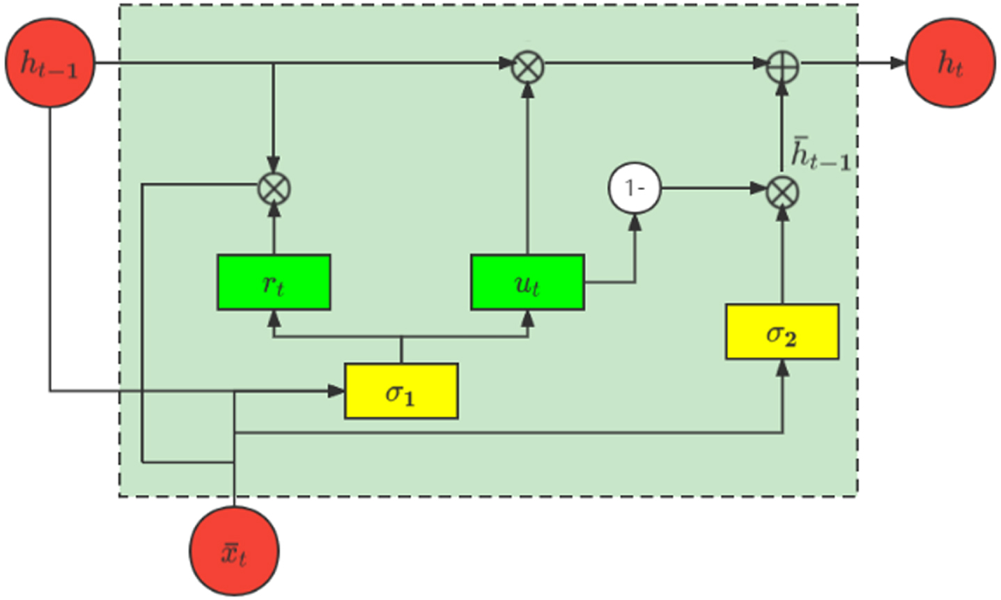u_t represents the update gate, which is used to control the extent of and the current traffic state ${\bar{x}}_{t}$ as input and finally obtains a new hidden state h_t. The formula of GRU is as follows: $u_{t} = σ (W_{u} \cdot [h_{t - 1}, X] + b_{u}),$ (4) $r_{t} = σ (W_{r} \cdot [h_{t - 1}, X] + b_{r}),$ (5) ${\hat{h}}_{t - 1} = \tanh (W_{h} \cdot [r_{t} * h_{t - 1}, X] + b_{h}),$ (6) $h_{t} = u_{t} * h_{t - 1} + (1 - u_{t}) * {\hat{h}}_{t - 1},$ (7) where W_u, W_r, and W_h respectively represent the update gate, reset gate and the weight of h_t-1, and b_u, b_r, b_h are the corresponding deviation values, which are all parameters to be learned.

Fig. 3

Structure of the gated recurrent unit.

4 Multi-feature two stage attention convolution network

4.1 MTA-CN

In this section we describe the structure of MTA-CN. Qin et al. [43] proposed the DARNN model on the time series prediction problem, inspired by the dual stage attention in the model, we propose MTA-CN. Figure 4(a) shows the structure of MTA-CN. Take m historical time series as input, the notation r represents the current time series. Extract the time series χ^r ∈ R^N×(n+1)*T with a historical time step of $χ_{main}^{r} \in R^{N \times T}$ . The time series $χ_{main}^{r} \in R^{N \times T}$ of the most recent T time step is used as the main feature, and the time series $χ_{s}^{r} \in R^{N \times nT}$ of the remaining nT length is used as the period feature. The subscript main and the subscript s represent the main feature and time period feature respectively. The model uses two T-GCNs following the encoder-decoder architecture [32]. In the encoder part, as shown in Fig. 4(b), we use time period attention so that the model can adaptively select relevant time period features and reweight them. In the decoder part, as shown in Fig. 4(c), temporal attention is used to select the hidden state for the relevant time step. After adding these two attention mechanisms, MTA-CN can adaptively capture long-term temporal correlation.

Fig. 4

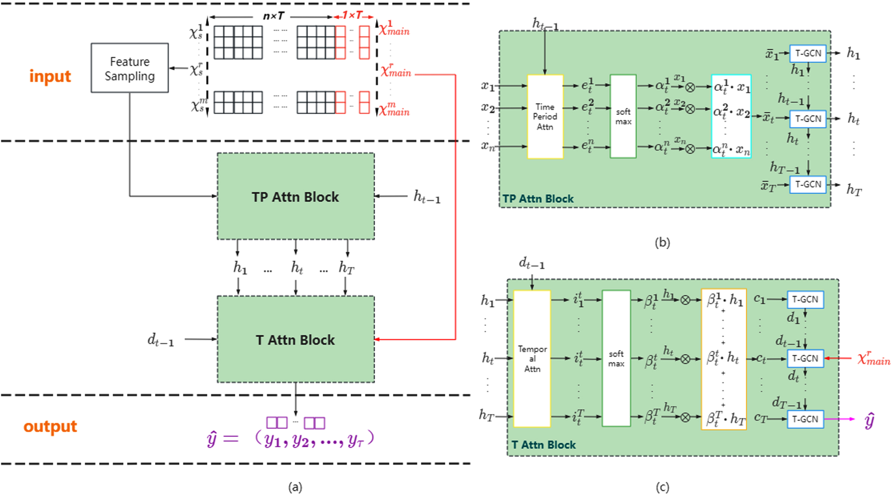
(a) MTA-CN overall architecture. (b) Encoder internal structure. (c) Decoder internal structure.

4.2 Feature sampling

Before the time series $χ_{s}^{r} \in R^{N \times nT}$ considered as a period feature enters the encoder, its dimension is converted into x = (x₁, x₂, …, x_n-1, x_n) ∈ R^N×T×n. We can regard this sequence as a time series with a time step of T, and each time step contains n time period features.

4.3 Time period attention on encoder

As shown in Fig. 4(b), the time series $χ_{s}^{r}$ passes through feature sampling to obtain a time series (x₁, x₂, …, x_n-1, x_n) ∈ R^N×T×n with a total number of features of n. Different time period features have different effects on the results of the next moment. We designed a time period attention to adaptively capture the dynamic correlation between different time periods, and assign different weights by calculating the correlation. We constructed a time period feature attention model by inputting time series x = (x₁, x₂, …, x_n-1, x_n) ∈ R^N×T×n and the previous hidden state h_t-1, the formulas are shown as follows: $e_{t}^{k} = v_{1} tanh (q_{1} h_{t - 1} + k_{1} x_{t}), 1 ⩽ k ⩽ n,$ (8) $α_{t}^{k} = \frac{exp (e_{t}^{k})}{Σ_{i = 1}^{η} exp (e_{t}^{i})},$ (9) where q₁ ∈ R^a×T (the notation a is the number of hidden layers of the encoder), k₁ ∈ R^T×T and v₁ ∈ R^T are the parameters to be learned during the training process. e_t ∈ R^N×n is normalized by softmax becomes α_t ∈ R^N×n, and $α_{t}^{k}$ represents the attention weight of the k-th time period feature at time step t. Multiplying these weights with x_k yields a new sequence $\bar{x} = (α_{t}^{1} \cdot x_{1}, α_{t}^{2} \cdot x_{2}, \dots, α_{t}^{n - 1} \cdot x_{n - 1}, α_{t}^{n} \cdot x_{n}) \in R^{N \times T \times n}$ input to the encoder T-GCN.

Through the encoder T-GCN unit, a new hidden state h_t ∈ R^N×T×a can be obtained. T-GCN is a combination of GCN and GRU models. Through formulas (2)–(7), it can be obtained as following formulas: $u_{t} = σ (W_{u} \cdot [h_{t - 1}, GCN ({\bar{x}}_{t}, A)] + b_{u}),$ (10) $r_{t} = σ (W_{r} \cdot [h_{t - 1}, GCN ({\bar{x}}_{t}, A)] + b_{r}),$ (11) ${\hat{h}}_{t - 1} = \tanh (W_{h} \cdot [r_{t} * h_{t - 1}, GCN ({\bar{x}}_{t}, A)] + b_{h}),$ (12) $h_{t} = u_{t} * h_{t - 1} + (1 - u_{t}) * {\hat{h}}_{t - 1},$ (13) where GCN represents the calculation process of the graph convolutional neural network. u_t and r_t represent the update gate and reset gate respectively. W_u, W_r, W_h represent the update gate, reset gate and the weight of ${\hat{h}}_{t - 1}$ respectively. b_u, b_r, b_h are corresponding deviation.

4.4 Temporal attention on decoder

The correlation between the current traffic situation of the node and the previous traffic situation changes nonlinearly with the time step. After passing through the encoder with time period attention, in the decoder part, as shown in Fig. 4(c), in order to adaptively capture Encoder-dependent hidden states, we use temporal attention to capture correlations across different time steps. The temporal attention model is constructed by the hidden state h_i (1 ⩽ i ⩽ T) obtained in the encoder and the previous hidden state d_t-1 of the decoder, the formulas are shown as follows: $i_{t}^{k} = v_{2} tanh (q_{2} d_{t - 1} + k_{2} h_{k}), 1 ⩽ k ⩽ T,$ (14) $β_{t}^{k} = \frac{exp (i_{t}^{k})}{Σ_{j = 1}^{T} exp (i_{t}^{j})},$ (15) where q₂ ∈ R^b×a (the notation b is the number of hidden layers of the decoder), k₂ ∈ R^a×a and v₂ ∈ R^a are the parameters to be learned during the training process. i_t ∈ R^N×T is normalized by softmax becomes β_t ∈ R^N×T, and $β_{t}^{k}$ represents the attention weight of the k-th time step. The attention weight $β_{t}^{k}$ is weighted and added to the hidden state to obtain the context vector c_t, the formula is as follows: $c_{t} = Σ_{k = 1}^{T} β_{t}^{k} h_{k},$ (16) where h_k represents the k-th hidden state.

Get (each time step has an independent context vector) and then combine it with the main feature $χ_{main}^{r} \in R^{N \times T}$ combined to get a new sequence . $y^{*} = W_{c x} [c_{t}^{'}; χ_{main}^{r}],$ (17)

where through linear transformation to get the input y^* ∈ R^N×T×1. W_cx ∈ R^(a+1)×1 is the training parameter in the linear transformation process.

In order to predict the final output $\hat{y}$ , the decoder also uses T-GCN to obtain a new hidden state d_t. $u_{t} = σ (W_{u} \cdot [d_{t - 1}, GCN (y^{*}, A)] + b_{u}),$ (18) $r_{t} = σ (W_{r} \cdot [d_{t - 1}, GCN (y^{*}, A)] + b_{r}),$ (19) ${\hat{d}}_{t - 1} = \tanh (W_{d} \cdot [r_{t} * d_{t - 1}, GCN (y^{*}, A)] + b_{d}),$ (20) $d_{t} = u_{t} * d_{t - 1} + (1 - u_{t}) * {\hat{d}}_{t - 1},$ (21) where GCN represents the calculation process of the graph convolutional neural network, u_t and r_t represent the update gate and reset gate respectively, W_u, W_r, W_d represent the update gate, reset gate and the weight of ${\hat{h}}_{t - 1}$ , b_u, b_r, b_d are the corresponding deviation value.

With temporal attention, the decoder can adaptively capture more important time steps. The context vector c_t ∈ R^N×a and the current hidden state d_t ∈ R^N×b are obtained by the decoder. The [c_t ; d_t] ∈ R^N×(a+b) formed by combining the two sets of sequences is a time series that simultaneously captures the time period features and the importance of time steps. We get the final output $\hat{y} \in R^{N \times τ}$ through two layers of linear transformation. $\hat{y} = W_{b} (W_{a} [c_{t}; d_{t}]),$ (22) where τ represents the time step to be predicted, W_a ∈ R^(a+b)×b, W_b ∈ R^b×τ are the training parameters in the linear transformation process.

The pseudo-code of MTA-CN is summarized as follows:

Algorithm: MTA-CN
Input: Adjacency matrix A∈R^N×N, time period features $χ_{s}^{r} \in R^{N \times nT}$ and main features $χ_{main}^{r} \in R^{N \times T}$ .
for i, i=1,2,..,m do
1 Get x=Feature Sampling( $χ_{s}^{r}$ );
2 Get α_t=TP Attn(x) by (8) (9);
3 Get $\bar{x}$ =( $α_{t}^{1} \cdot x_{1}, α_{t}^{2}, \dots, α_{t}^{n - 1} \cdot x_{n - 1}, α_{t}^{n} \cdot x_{n}$ );
4 Get h_t=GCN-GRU( $\bar{x}, A$ ) by (10) (11) (12) (13);
5 Get β_t=T Attn(h_t) by (14) (15);
6 Get $c_{t} = Σ_{k = 1}^{T} β_{t}^{k} h_{k}$ by (16);
7 Get y^*=MLP () by (17);
8 Get $\hat{y}$ = MLP(MLP(GCN-GRU (y^*, A))) by (18) (19) (20) (21) (22);
end for
return $\hat{y}$ .
Output: final predicted value $\hat{y}$ .

5 Experiments

5.1 Dataset

To assess the performance of our model, we conducted experiments on two real-world datasets: Los Angeles Expressway (Los-loop) and Shenzhen Luohu District Taxi (Sz-taxi).

Los-loop: Traffic speed collected by 207 sensors on the Los Angeles Freeway from March 1st to March 7th, 2012. The sensors record the traffic speed every five minutes. The total number of time slices is 2016.

Sz-taxi: The trajectory data of taxis in Luohu District, Shenzhen, from January 1st to January 31st, 2015. It includes 156 main roads in the area, and the traffic speed is recorded every 15 minutes. The total number of time slices is 2976.

For the above two datasets, we divide the first 80% as the training set, 10% as the validation set, and the last 10% as the test set.

5.2 Hyperparameters

The hardware environment of this experiment is CPU: 11th Gen Intel(R) Core(TM) i7-11800H @ 2.30 GHz, GPU:NVDIA GeForce RTX 3060 6G.

The software environment is: windows10, python 3.9.12, torch version 1.12.0.

In terms of hyperparameters, we set the learning rate to 0.001, the batch size to 16, the number of iterations to 500, the hidden layer size of the encoder and decoder to a=b=128, and the number of time period features n= 23. In order to improve the convergence speed of the model, we normalize the samples in the interval [0,1]. Because the recording intervals of the two data sets are different, we set the historical time step T_l of the data set Los-loop to (n+1)*12, and the historical time step T_s of the data set Sz-taxi to (n+1)*4, to predict the traffic speed in the next 15 minutes, 30 minutes, 45 minutes and 60 minutes. Therefore, the prediction steps τ_l of the data set Los-loop are (3,6,9,12), and the prediction steps τ_s of the data set Sz-taxi are (1,2,3,4). Finally, we use adam optimizer to train our model.

5.3 Evaluation metrics

We use four evaluation metrics to evaluate the performance of MTA-CN.

Mean Absolute Error (MAE): MAE can well reflect the actual situation of the predicted value error, and the smaller the MAE, the better the model performance. $MAE = \frac{1}{NM} Σ_{i = 1}^{N} Σ_{j = 1}^{M} | y_{j}^{i} - {\hat{y}}_{j}^{i} | .$ (23)

Root Mean Squared Error (RMSE): RMSE is used to measure the deviation between the true value and the predicted value. The closer the predicted value is to the actual value, the smaller the root mean square error between the two. The smaller the RMSE, the better the model performance. $RMSE = \sqrt{\frac{1}{NM} Σ_{i = 1}^{N} Σ_{j = 1}^{M} {(y_{j}^{i} - {\hat{y}}_{j}^{i})}^{2}} .$ (24)

Coefficient of Determination (R²): R² is a measure of the goodness of fit of the estimated regression equation. The closer R² is to 1, the better the fit and the better the performance of the model. $R^{2} = 1 - \frac{Σ_{i = 1}^{N} Σ_{j = 1}^{M} {(y_{j}^{i} - {\hat{y}}_{j}^{i})}^{2}}{y Σ_{i = 1}^{N} Σ_{j = 1}^{M} {(y_{j}^{i} - \bar{Y})}^{2}} .$ (25)

Explained Variance Score (var): var is used to measure the degree to which the model can explain the fluctuation of the data set. When the result is closer to 1, the model performance is better. $var = 1 - \frac{Var {Y - \hat{Y}}}{Var {Y}},$ (26) where $y_{j}^{i}$ and ${\hat{y}}_{j}^{i}$ represent the actual value and predicted value of the j-th time sample of the i-th node, respectively, and N and M represent the number of nodes and the number of time samples in the test set, respectively. Y and $\hat{Y}$ represent the collection of $y_{j}^{i}$ and ${\hat{y}}_{j}^{i}$ respectively. $\bar{Y}$ represents the mean value of Y, and Var represents the variance.

5.4 Experimental results

In this paper, the following baseline models are selected for comparison with MTA-CN.

Support Vector Regression (SVR) [16]: SVR are suitable for small sample data and can solve high-dimensional problems.

Autoregressive Integrated Moving Average model (ARIMA) [14]: ARIMA can make dynamic prediction by using the dependencies and correlations between time series observations

Gated Recurrent Unit model (GRU) [21]: GRU is a variant of RNN that can capture dependencies with large intervals in time series data.

Graph Convolutional Network model (GCN) [33]: GCN extends the convolution operation to the graph structure, considering the spatial structure.

A Temporal Graph Convolutional Network (T-GCN) [32]: A hybrid model that uses GCN to extract spatial structure features and GRU to extract temporal features.

Attention Temporal Graph Convolutional Network (A3T-GCN) [44]: On the basis of T-GCN, an attention mechanism is added to extract the weight of the time step.

Table 2 shows the performance results of the MTA-CN model and other baseline models predicting the next 15 minutes, 30 minutes, 45 minutes, and 60 minutes on the Los-loop dataset and the Sz-taxi dataset. (*) indicates values too small to be statistically significant. Our proposed model outperforms most of the baseline models in both datasets. Based on the results, we draw the following conclusions.

Table 2
Comparison of prediction results between MTA-CN and other baseline models

T Metric Los-loop

SVR ARIMA GRU GCN T-GCN A3T-GCN MTA-CN

15min RMSE 6.1263 11.3737 5.5522 8.3343 5.5280 5.6073 5.5659

MAE 3.9472 6.9202 3.3542 5.9223 3.5432 3.6544 3.4781

R² 0.7596 * 0.7874 0.5045 0.7949 0.7900 0.7878

var 0.7579 * 0.7958 0.5094 0.7955 0.7947 0.7907

30min RMSE 7.0598 11.6587 6.6498 8.8961 6.6200 6.6646 6.5304

MAE 4.2031 7.3974 3.9841 6.2612 4.3018 4.3039 4.0484

R² 0.7134 * 0.7207 0.4610 0.7227 0.7188 0.7292

var 0.7128 * 0.7321 0.4671 0.7279 0.7251 0.7385

45min RMSE 8.1811 11.4326 7.5211 9.3845 7.6290 7.7043 7.2326

MAE 4.6727 7.1499 4.6129 6.6469 5.0060 5.0634 4.5405

R² 0.6049 * 0.6575 0.4199 0.6383 0.6346 0.6831

var 0.5803 * 0.6727 0.4264 0.6483 0.6457 0.6917

60min RMSE 9.1411 11.4495 8.3360 9.9084 8.3608 8.4082 7.7905

MAE 5.1531 7.3049 5.1420 7.1500 5.4781 5.5628 4.8951

R² 0.5154 * 0.5893 0.3774 0.5753 0.5737 0.6370

var 0.4677 * 0.6070 0.3849 0.5868 0.5874 0.6444

T Metric Sz-taxi

SVR ARIMA GRU GCN T-GCN A3T-GCN MTA-CN

15min RMSE 4.3085 10.0481 4.3656 5.4699 4.2761 4.2574 4.1440

MAE 2.9264 8.2690 2.9347 4.0001 2.9349 2.9266 2.8105

R² 0.8316 * 0.8254 0.7271 0.8324 0.8338 0.8426

var 0.8317 * 0.8256 0.7272 0.8326 0.8341 0.8430

30min RMSE 4.3286 9.1784 4.4132 5.4965 4.3136 4.3179 4.1684

MAE 2.8924 7.4267 2.9531 4.0210 2.9610 2.9842 2.8158

R² 0.8301 * 0.8216 0.7244 0.8294 0.8291 0.8407

var 0.8305 * 0.8217 0.7246 0.8297 0.8294 0.8412

45min RMSE 4.3532 8.9243 4.4480 5.5175 4.3831 4.4168 4.2160

MAE 2.9423 7.0801 2.9828 4.0393 3.0501 3.0755 2.8954

R² 0.8281 * 0.8187 0.7223 0.8240 0.8212 0.8371

var 0.8290 * 0.8189 0.7226 0.8244 0.8215 0.8375

60min RMSE 4.5113 8.5287 4.4890 5.5392 4.3584 4.4457 4.2637

MAE 3.0824 6.6341 3.0275 4.0568 3.0318 3.0980 2.9396

R² 0.8259 * 0.8153 0.7202 0.8261 0.8189 0.8334

var 0.8272 * 0.8157 0.7205 0.8273 0.8192 0.8340

T	Metric	Los-loop
15min	RMSE	6.1263	11.3737	5.5522	8.3343	5.5280	5.6073	5.5659
	MAE	3.9472	6.9202	3.3542	5.9223	3.5432	3.6544	3.4781
	R²	0.7596	*	0.7874	0.5045	0.7949	0.7900	0.7878
	var	0.7579	*	0.7958	0.5094	0.7955	0.7947	0.7907
30min	RMSE	7.0598	11.6587	6.6498	8.8961	6.6200	6.6646	6.5304
	MAE	4.2031	7.3974	3.9841	6.2612	4.3018	4.3039	4.0484
	R²	0.7134	*	0.7207	0.4610	0.7227	0.7188	0.7292
	var	0.7128	*	0.7321	0.4671	0.7279	0.7251	0.7385
45min	RMSE	8.1811	11.4326	7.5211	9.3845	7.6290	7.7043	7.2326
	MAE	4.6727	7.1499	4.6129	6.6469	5.0060	5.0634	4.5405
	R²	0.6049	*	0.6575	0.4199	0.6383	0.6346	0.6831
	var	0.5803	*	0.6727	0.4264	0.6483	0.6457	0.6917
60min	RMSE	9.1411	11.4495	8.3360	9.9084	8.3608	8.4082	7.7905
	MAE	5.1531	7.3049	5.1420	7.1500	5.4781	5.5628	4.8951
	R²	0.5154	*	0.5893	0.3774	0.5753	0.5737	0.6370
	var	0.4677	*	0.6070	0.3849	0.5868	0.5874	0.6444
T	Metric	Sz-taxi
		SVR	ARIMA	GRU	GCN	T-GCN	A3T-GCN	MTA-CN
15min	RMSE	4.3085	10.0481	4.3656	5.4699	4.2761	4.2574	4.1440
	MAE	2.9264	8.2690	2.9347	4.0001	2.9349	2.9266	2.8105
	R²	0.8316	*	0.8254	0.7271	0.8324	0.8338	0.8426
	var	0.8317	*	0.8256	0.7272	0.8326	0.8341	0.8430
30min	RMSE	4.3286	9.1784	4.4132	5.4965	4.3136	4.3179	4.1684
	MAE	2.8924	7.4267	2.9531	4.0210	2.9610	2.9842	2.8158
	R²	0.8301	*	0.8216	0.7244	0.8294	0.8291	0.8407
	var	0.8305	*	0.8217	0.7246	0.8297	0.8294	0.8412
45min	RMSE	4.3532	8.9243	4.4480	5.5175	4.3831	4.4168	4.2160
	MAE	2.9423	7.0801	2.9828	4.0393	3.0501	3.0755	2.8954
	R²	0.8281	*	0.8187	0.7223	0.8240	0.8212	0.8371
	var	0.8290	*	0.8189	0.7226	0.8244	0.8215	0.8375
60min	RMSE	4.5113	8.5287	4.4890	5.5392	4.3584	4.4457	4.2637
	MAE	3.0824	6.6341	3.0275	4.0568	3.0318	3.0980	2.9396
	R²	0.8259	*	0.8153	0.7202	0.8261	0.8189	0.8334
	var	0.8272	*	0.8157	0.7205	0.8273	0.8192	0.8340

Deep learning-based methods are more effective than traditional machine learning methods on the two datasets. Traditional methods have limited ability to model non-linear and complex traffic data. For example, the ARIMA model requires stable data, but due to the complexity of real-life traffic situations and the many influencing factors, ARIMA performs poorly compared to other baseline models. Due to the ever-increasing amount of data, traditional machine learning approaches are increasingly challenged to outperform data-driven deep learning models in terms of performance. In contrast, deep learning-based methods can model nonlinear data and consider the topology of the traffic network, leading to higher accuracy. Among them, MTA-CN has more advanced performance than other models. In order to prove that MTA-CN can not only consider temporal and spatial correlations, but also learn temporal patterns from long-term time series, we compare the MTA-CN model with GRU, GCN, T-GCN, and A3T-GCN, as shown in Figs. 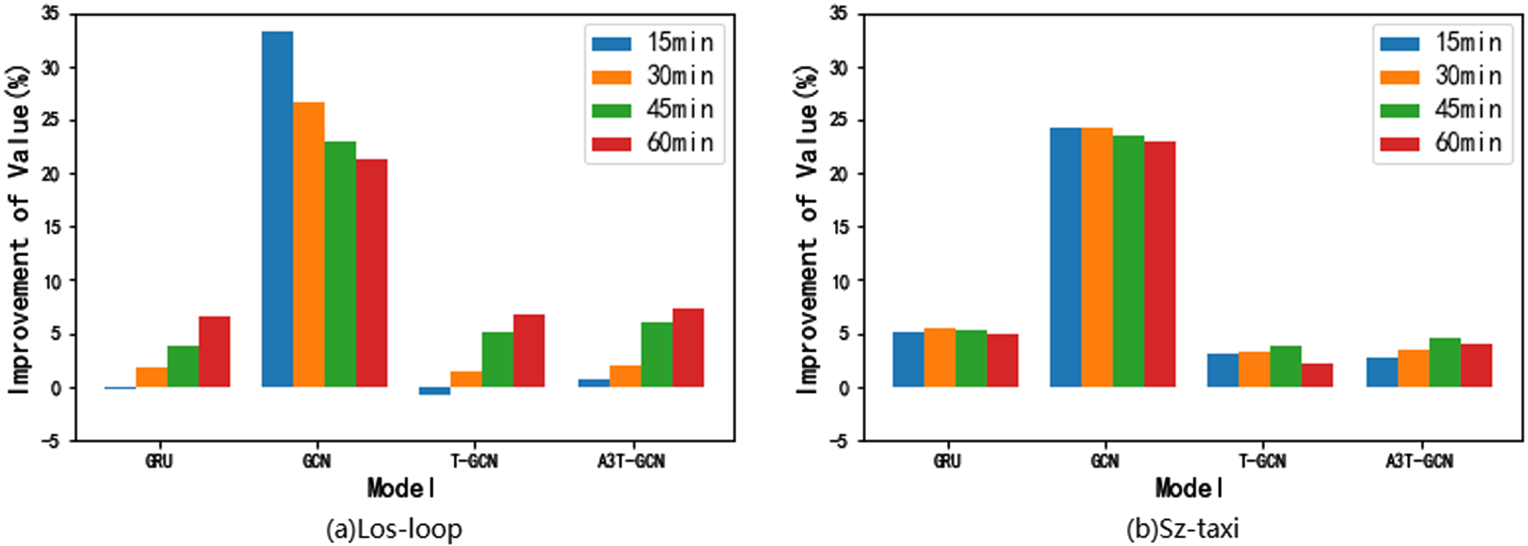5 and 6, they represent the improvement percentage of our model compared to some other deep learning baseline models on the two evaluation indicators RMSE and MAE, the calculation formula is as follows: $\frac{B - A}{B},$ (27) where A represents the value of MTA-CN, and B represents the value of the baseline model.

Fig. 5

Percentage improvement of MTA-CN compared to other deep learning baseline models on RMSE metric for different prediction steps.

Fig. 6

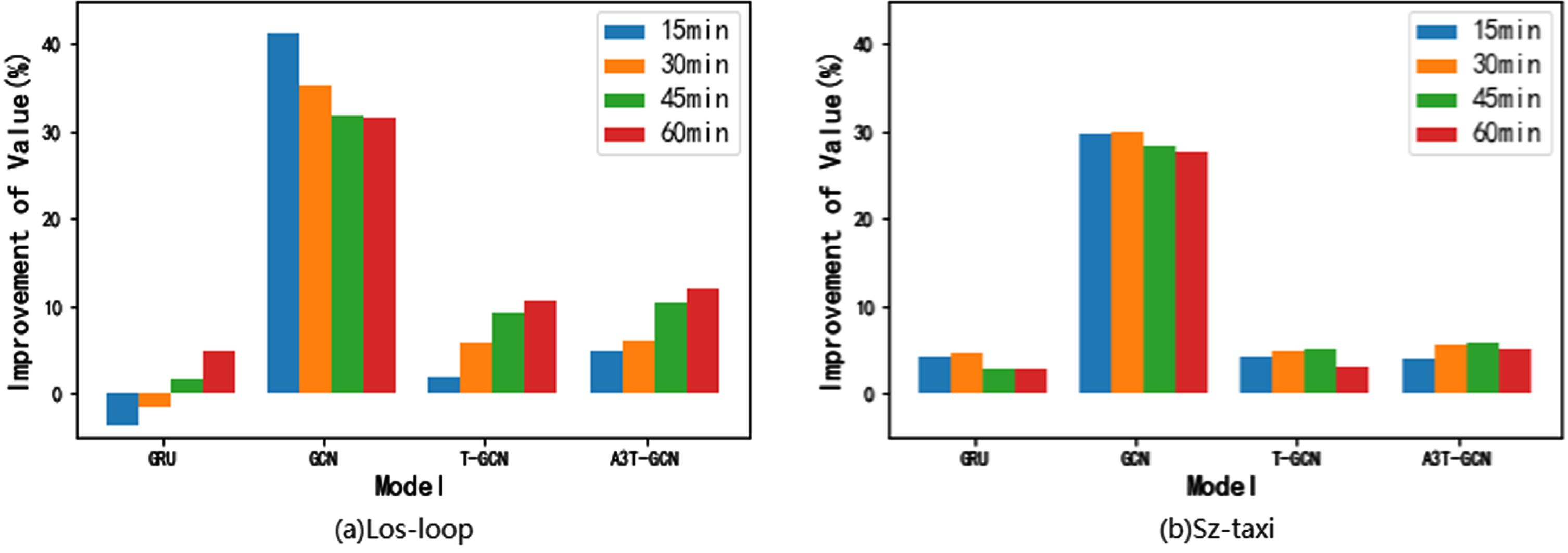
Percentage improvement of MTA-CN compared to other deep learning baseline models on MAE metric for different prediction steps.

In the 60-minute prediction of the two datasets, MTA-CN outperformed several models in terms of the improvement percentage of RMSE and MAE indicators. Compared to the GRU, MTA-CN achieved approximately 6.54% and 5.02% improvement in the RMSE metric, and approximately 4.8% and 2.9% improvement in the MAE metric. This is because the GRU model only aggregates temporal features without considering spatial features. Compared to the GCN, MTA-CN achieved approximately 21.37% and 23.02% improvement in the RMSE metric, and approximately 31.54% and 27.54% improvement in the MAE metric. The significant difference in performance is due to the fact that GCN only aggregates spatial features without considering temporal features. As a model based on spatiotemporal features, MTA-CN exhibits better predictive accuracy than GRU and GCN, which only consider single factors.

Compared to T-GCN, which is based on spatiotemporal features, MTA-CN has achieved an improvement of approximately 6.82% and 2.17% in terms of RMSE, and approximately 10.64% and 3.04% in terms of MAE. Compared to T-GCN, MTA-CN not only considers spatio-temporal features, but also utilizes an attention mechanism to select more important temporal features for prediction. As a consequence, MTA-CN achieves better prediction performance.

A3T-GCN not only considers spatio-temporal features but also captures the correlation of temporal features, assigning higher weights to more important temporal features. Compared to A3T-GCN, MTA-CN achieves improvements of approximately 7.34% and 4.09% in RMSE, and approximately 12% and 5.11% in MAE, respectively. This is because MTA-CN takes into account longer-term temporal features and aggregates them into a special sequence, resulting in higher accuracy.

However, for some lower prediction steps, MTA-CN’s prediction accuracy was slightly inferior to some baseline models. For example, in the 15-minute prediction and 30-minute prediction on the Los-loop dataset, the prediction accuracy of MTA-CN was not as good as GRU and T-GCN. Nevertheless, at high prediction steps, MTA-CN achieved better accuracy than other baseline models, indicating that our model is more suitable for long-term prediction.

In order to test the long-term prediction ability of the model, we plotted the trend of two evaluation indices as the prediction step size increases for each model. Although some models that only consider time correlation can achieve better results in short-term prediction, the prediction difficulty increases as the prediction interval increases, resulting in a decrease in accuracy. This is because errors stack up with each prediction and become larger as the interval increases. As shown in Fig. 7, SVR, GRU, T-GCN, and A3T-GCN perform well in short-term prediction on the Los-loop dataset, but their accuracy sharply declines as the interval increases. The accuracy of MTA-CN declined relatively slowly. In the Sz-taxi dataset (Fig. 8), the accuracy decline trend of these models is relatively stable due to the different measurement intervals of the two datasets. This is due to the different measurement intervals between the two data sets, the measurement interval of Sz-taxi is 15 minutes, and the measurement interval of Los-loop is 5 minutes, so the prediction steps corresponding to Los-loop are 3, 6, 9, 12 respectively, while the prediction steps corresponding to the SZ-taxi data set are only 1, 2, 3, 4. In conclusion, our model MTA-CN demonstrates excellent long-term prediction ability with minimal change in prediction results as the prediction step size varies. Therefore, it can be used for both short-term and long-term prediction.

Fig. 7

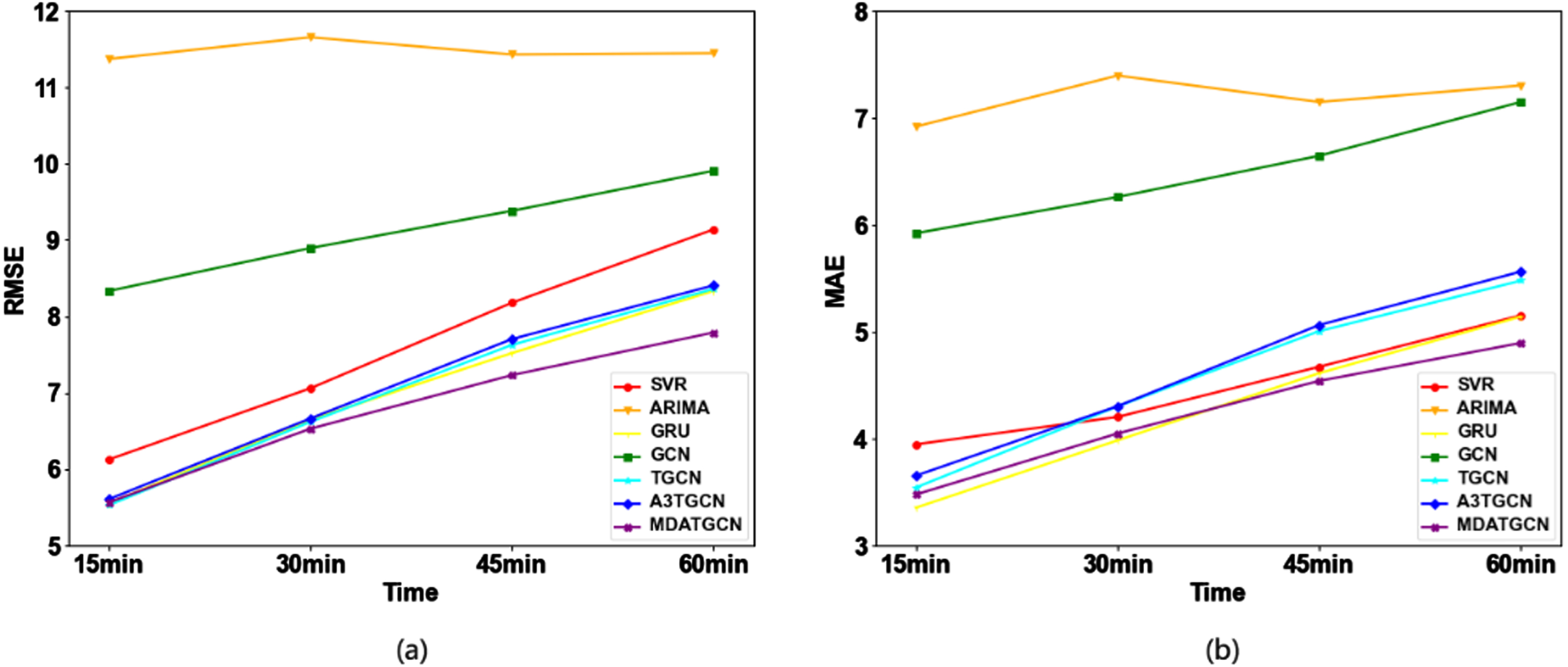
Under different prediction steps. (a) Changes in the evaluation index RMSE on the Los-loop dataset. (b) Changes in the evaluation index MAE on the Los-loop dataset.

Fig. 8

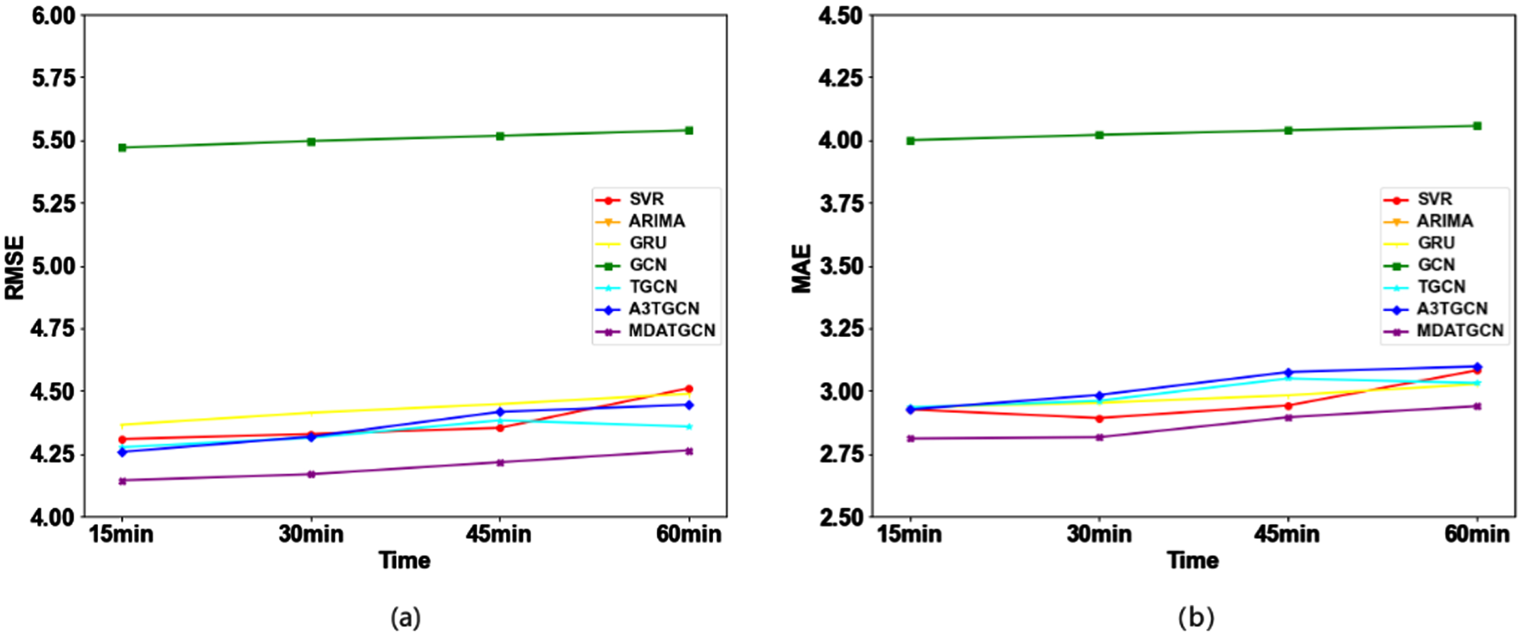
Under different prediction steps. (a) Changes in the evaluation index RMSE on the Sz-taxi dataset. (b) Changes in the evaluation index MAE on the Sz-taxi dataset.

To assess whether MTA-CN captures long-term temporal features, we introduce additional noise sequences to the dataset. Specifically, we add a noise sequence of equal length to the time period feature in the Los-loop dataset and the Sz-taxi dataset. Then we input these sequences into the MTA-CN model. In this paper, the historical time step is denoted as (n+1)T, where n=23 represents the 23 time period features in the encoder. We add 23 additional time series of length T to the input time series, which are randomly distributed between [0,1]. Figure 9(a) and (b) show the weight distributions of 46 sequences, where the first 23 represent the original sequence, and the last 23 represent the noise sequence. We use all 46 sequences as input and apply the attention network to scale these weights. Our results demonstrate that the attention mechanism assigns larger weights to the original sequence and smaller weights to the noisy sequence, indicating that MTA-CN adaptively selects more relevant time period features and captures longer temporal correlations. Therefore, our model not only exhibits excellent predictive performance, but also demonstrates interpretability advantages.

Fig. 9

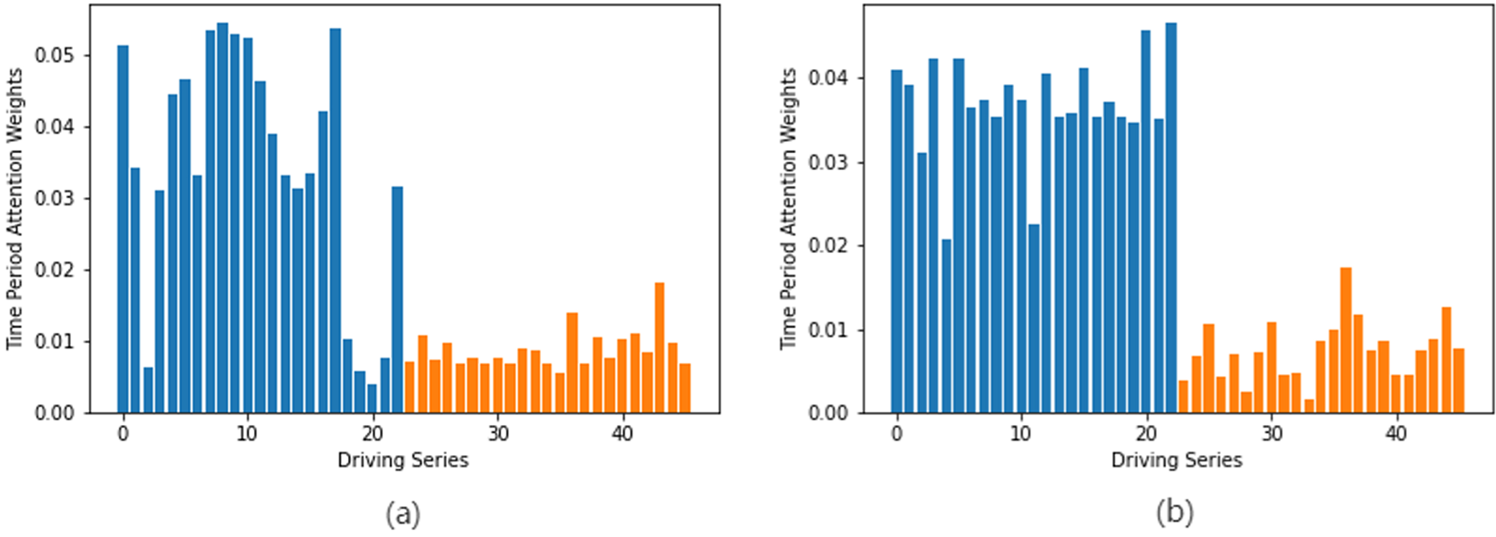
Time period feature attention weight map, the first twenty-three represent real time period features, and the last twenty-three represent added noise sequences. (a) Los-loop. (b) Sz-taxi.

5.5 Visualization results

To gain a better understanding of MTA-CN, we selected a road from the Los-loop dataset and the Sz-taxi dataset respectively and visualized the prediction results of the test set. In Fig. 10(a)–(d) illustrate the prediction results of 15 minutes, 30 minutes, 45 minutes, and 60 minutes on the Los-loop test set, respectively. In Fig. 11(a)–(d), we find the prediction results of 15 minutes, 30 minutes, 45 minutes, and 60 minutes on the Sz-taxi test set, respectively.

Fig. 10

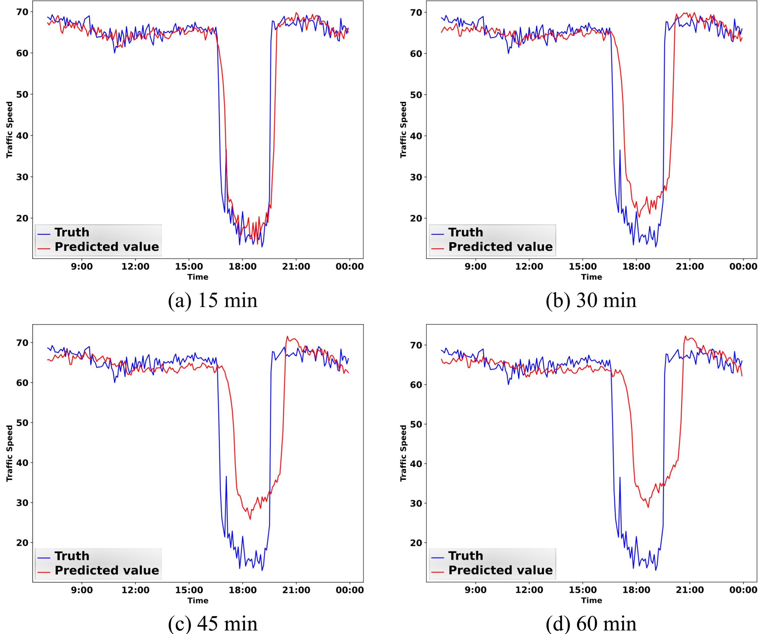
Visualization of different prediction steps on the Los-loop test set.

Fig. 11

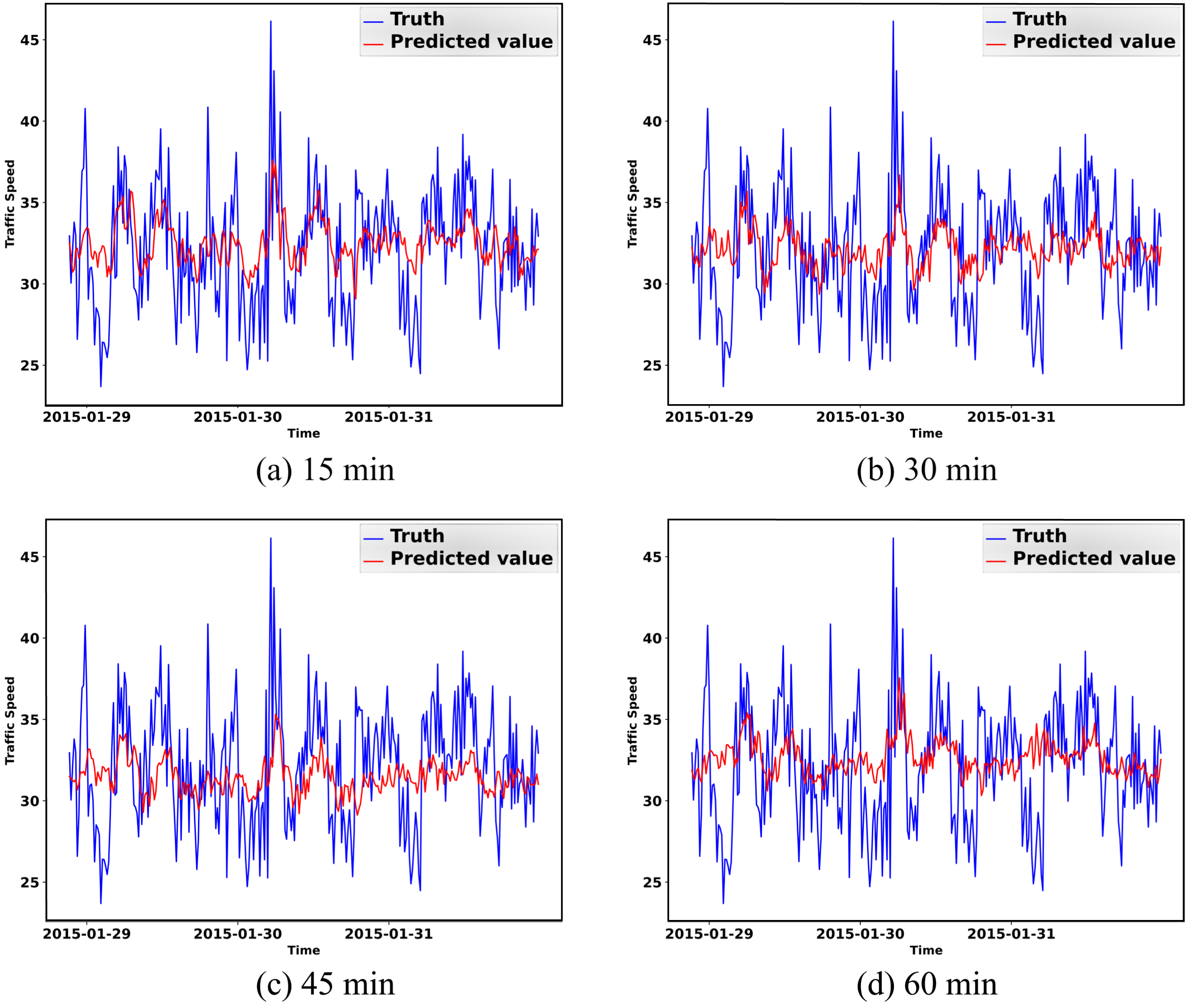
Visualization of different prediction steps on the Sz-taxi test set.

We observed that short-term predictions on the same dataset were better than long-term predictions. In the Los-loop dataset, the prediction accuracy for the 15-minute interval was high, but as the prediction interval increased, the accuracy of the model in some time periods with significant changes in actual values decreased, such as 15 : 00–21 : 00. However, in relatively stable periods, such as 9 : 00-15 : 00, the prediction accuracy was not significantly affected despite the accumulation of errors. In periods with more significant changes, errors accumulated more, leading to decreased prediction accuracy. Moreover, analysis of the prediction results in the Sz-taxi dataset showed that the model’s prediction accuracy for local maximum and minimum values was poor, which was attributed to the over-smoothing problem of GCN during training.

Despite these limitations, the MTA-CN model was able to capture the temporal and spatial variation trends of the road and produce relatively good prediction results, indicating its effectiveness in traffic speed prediction.

6 Conclusions

We proposed a MTA-CN for traffic speed prediction, which network comprises an encoder with time period feature attention and a decoder with temporal attention. The time period feature attention mechanism enables the encoder to selectively identify relevant time period features, while the temporal attention mechanism allows the decoder to adaptively capture correlations at different time steps. Instead of the traditional recurrent neural network, we used a Temporal Graph Convolutional Network (T-GCN), which integrates Graph Convolutional Neural Network (GCN) and Gated Recurrent Unit (GRU) to capture the topology of non-Euclidean space and the dynamic changes of node traffic information. The spatio-temporal correlation of traffic road networks can be fully considered by T-GCN, and based on two attention mechanisms, MTA-CN can learn the correlation from long-term time series. MTA-CN performs better in almost all of the different prediction ranges when using it to compare with other baseline models on two real world datasets. The model we proposed successfully extracts spatial features and long-term temporal features from the traffic information.

In the future works, the model proposed in this paper could be improved in the several directions, such as contribute to the progress of efficiently predicting the peak hours or road accidents in the studied traffic network. We only use GCN to extract spatial features. Building on the foundation of this study, replacing GCN with other advanced graph neural networks may lead to improved research outcomes.

Footnotes

Acknowledgments

This work was supported in part by Fujian Provincial Department of Science and Technology under Grant No. 2021J011070, and Fujian University of Technology under Grant No. GY-Z18148.

References

Hung

M.H.

, Wang

C.H.

and He

, A Real-Time Routing Algorithm for End-to-End Communication Networks with QoS Requirements, Proceedings of the 3rd International Conference on Computing, Measurement, Control and Sensor Network (CMCSN2016), (2016), 186–189.

Wang

C.H.

, Chung

W.H.

, Lee

C.J.

and Wu

M.E.

, An atomic routing game for multi-class communication networks with quality of service requirements, 2015 24th Wireless and Optical Communication Conference (WOCC), (2015), 206–210.

Wang

C.H.

, Wu

M.E.

and Chung

W.H.

, Perspectives of Bandwidth Sharing Schemes in Communication Systems with Blocking, Proceedings of the ASE Big Data & Social Informatics 2015, October 7-9, 2015.

Wang

C.H.

and Luh

H.P.

, Analysis of bandwidth allocation on end-to-end QoS networks under budget control. Computers & Mathematics with Applications 62(1) (2011), 419–439.

Wang

C.H.

, Chen

, Zhao

and Suo

, An Efficient End-to-End Obstacle Avoidance Path Planning Algorithm for Intelligent Vehicles Based on Improved Whale Optimization Algorithm. Mathematics 11 (2023), 1800.

Wang

C.H.

, Chen

Y.T.

and Wu

, A Multi-Tier Inspection Queueing System with Finite Capacity for Differentiated Border Control Measures, IEEE Access 9 (2021), 60489–60502.

Wang

C.H.

and Wu

, Performance analysis of a security-check system with four types of inspection channels for high-speed rail stations in China. INFORMS International Conference on Service Science. Springer, Cham, (2019), 7–16.

Wang

C.H.

, Arena simulation for aviation passenger security-check systems. International Conference on Genetic and Evolutionary Computing, Springer, Cham, (2016), 95–102.

Dong

, Research on the Industrial Development of Intelligent Transportation System in China, 2020 5th International Conference on Electromechanical Control Technology and Transportation (ICECTT), (2020), 622–627.

10.

Jiang

and Luo.

, Graph neural network for traffic forecasting: A survey, Expert Systems with Applications 117921 (2022).

11.

Cho

, Van Merriënboer

, Bahdanau

and Bengio

, On the properties of neural machine translation: Encoder-decoder approaches, Sep. 2014, arXiv:1409.1259. [Online], Available: https://arxiv.org/abs/1409.1259

12.

Guo

, Lin

, Feng

, Song

and Wan

, Attention based spatial-temporal graph convolutional networks for traffic flow forecasting, Proceedings of the AAAI conference on artificial intelligence, 33(1) (2019), 922–929.

13.

Liu

and Guan

, A summary of traffic flow forecasting methods, Journal of highway and transportation research and development, vol. 21(3) (2004), 82–85.

14.

Hamed

MM.

, Al-Masaeid

HR.

and Said

ZMB.

, Short-term prediction of traffic volume in urban arterials, Journal of Transportation Engineering 121(3) (1995), 249–254.

15.

Zivot

and Wang

, Vector autoregressive models for multivariate time series, Modeling financial time series with S-PLUS® (2006), 385–429.

16.

Smola

A.J.

and Schölkopf

, A tutorial on support vector regression. Statist. Comput 14(3) (2004), 199–222.

17.

Sun

, Zhang

and Yu

, A Bayesian network approach to traffic flow forecasting, IEEE Transactions on Intelligent Transportation Systems 7(1) (2006), 124–132.

18.

Okutani

and Stephanedes

Y.J.

, Dynamic prediction of traffic volume through Kalman filtering theory, Transportation Research Part B: Methodological 18(1) (1984), 1–11.

19.

Kumar

and Raubal

, Applications of deep learning in congestion detection, prediction and alleviation: A survey, Transportation Research Part C: Emerging Technologies 133 (2021), 103432.

20.

Hochreiter

and Schmidhuber

, Long short-term memory, –, Neural Computation 9(8) (1735), 1780.

21.

Shahbazi

and Byun

Y.C.

, Topic modeling in short-text using non-negative matrix factorization based on deep reinforcement learning, Journal of Intelligent & Fuzzy Systems 39(1) (2020), 753–770.

22.

Wang

C.H.

, Wu

and Chen

Y.T.

, An empirical analysis for forecasting stock index based on lstm neural network, Proceedings of the 2021 5th International Conference on Electronic Information Technology and Computer Engineering, (2021), 636–641.

23.

, Predicting short-term traffic flow in urban based on multivariate linear regression model, Journal of Intelligent & Fuzzy Systems 39(2) (2020), 1417–1427.

24.

Liu

, Zheng

, Feng

and Chen

, Short-term traffic flow prediction with Conv-LSTM, 2017 9th International Conference on Wireless Communications and Signal Processing (WCSP). IEEE (2017), 1–6.

25.

Zhang

, Zheng

, Sun

and Qi

, Flow prediction in spatio-temporal networks based on multitask deep learning, IEEE Transactions on Knowledge and Data Engineering 32(3) (2020), 468–478.

26.

Chen

, Chen

, Ren

, Wu

and Yao

, Poster: Deeptfp: Mobile time series data analytics based traffic flow prediction. In Proceedings of the 23rd Annual International Conference on Mobile Computing and Networking, (2017), 537–539.

27.

Ranjan

, Bhandari

, Zhao

H.P.

, Kim

and Khan

, City-wide traffic congestion prediction based on CNN, LSTM and transpose CNN, IEEE Access 8 (2020), 81606–81620.

28.

Cheng

, Zhang

, Zhou

and Xu

, Deeptransport: Learning spatial-temporal dependency for traffic condition forecasting, 2018 International Joint Conference on Neural Networks (IJCNN). IEEE (2018), 1–8.

29.

Wang

, Yan

, Lu

, Zhang

and Li

, Explore uncertainty in residual networks for crowds flow prediction. 2018 International Joint Conference on Neural Networks (IJCNN). IEEE (2018), 1–7.

30.

Chai

, Wang

and Yang

, Bike flow prediction with multi-graph convolutional networks, Proceedings of the 26th ACM SIGSPATIAL international conference on advances in geographic information systems, (2018), 397–400.

31.

, Yu

, Shahabi

and Liu

, Diffusion convolutional recurrent neural network: Data-driven traffic forecasting, July. 2017, arXiv:1707.01926. [Online], Available: https://arxiv.org/abs/1707.01926

32.

Zhao

, Song

, Zhang

, Liu

, Wang

, Lin

and Li

, T-gcn: A temporal graph convolutional network for traffic prediction, IEEE Transactions on Intelligent Transportation Systems 21(9) (2020), 3848–3858.

33.

Welling

and Kipf

T.N.

, Semi-supervised classification with graph convolutional networks, J. International Conference on Learning Representations (ICLR 2017) 2016.

34.

, Yin

and Zhu

, Spatio-temporal graph convolutional networks: A deep learning framework for traffic forecasting. Sep. 2017, arXiv:1709.04875. [Online], Available: https://arxiv.org/abs/1709.04875.

35.

Vaswani

, Shazeer

, Parmar

, Uszkoreit

, Jones

, Gomez

A.N.

and Polosukhin

, Attention is all you need, Advances in Neural Information Processing Systems, 2017.

36.

Zheng

, Fan

, Wang

and Qi

, Gman: A graph multi-attention network for traffic prediction, Proceedings of the AAAI Conference on Artificial Intelligence 34(1) (2020), 1234–1241.

37.

Liang

, Ke

, Zhang

, Yi

and Zheng

, Geoman: Multi-level attention networks for geo-sensory time series prediction, IJCAI 2018 (2018), 3428–3434.

38.

Abdelraouf

, Abdel-Aty

and Yuan

, Utilizing attention-based multi-encoder-decoder neural networks for freeway traffic speed prediction, IEEE Transactions on Intelligent Transportation Systems 23(8) (2022), 11960–11969.

39.

Shao

, Zhang

, Wang

and Xu

, Pre-training Enhanced Spatial-temporal Graph Neural Network for Multivariate Time Series Forecasting, Proceedings of the 28th ACM SIGKDD Conference on Knowledge Discovery and Data Mining, (2022), 1567–1577.

40.

, Ge

, Song

, Jiang

, Zhou

and Qin

, A temporal-aware lstm enhanced by loss-switch mechanism for traffic flow forecasting, Neurocomputing 427 (2021), 169–178.

41.

Pan

, Hou

and Li

, Traffic Speed Prediction Based on Time Classification in Combination With Spatial Graph Convolutional Network, IEEE Transactions on Intelligent Transportation Systems, 2022.

42.

Chung

, Gulcehre

, Cho

and Bengio

, Empirical evaluation of gated recurrent neural networks on sequence modeling, Dec. 2014, arXiv: 1412.3555. [Online], Available: https://arxiv.org/abs/1412.3555.

43.

Qin

, Song

, Cheng

, Jiang

and Cottrell

, A dual-stage attention-based recurrent neural network for time series prediction, Proceedings of the 26th International Joint Conference on Artificial Intelligence, (2017), 2627–2633.

44.

Bai

, Zhu

, Song

, Zhao

, Hou

, Du

and Li

, A3t-gcn: Attention temporal graph convolutional network for traffic forecasting, ISPRS International Journal of Geo-Information 10(7) (2021), 485.