Hidden Markov model-based modeling and prediction for implied volatility surface 1

Abstract

The implied volatility plays a pivotal role in the options market, and a collection of implied volatilities across strike and maturity is known as the implied volatility surface (IVS). To capture the dynamics of IVS, this study examines the latent states of IVS and their relationship based on the regime-switching framework of the hidden Markov model (HMM). The cross-sectional models are first built for daily implied volatilities, and the obtained regression factors are regarded as the proxies of the IVS. Then, having these latent factors, the HMM is employed to model the dynamics of IVS. Take the advantages of HMM, the hidden state for each daily data is identified to achieve the corresponding time distribution, the characteristics, and the transition between the hidden states. The empirical study is conducted on the Shanghai 50ETF options, and the analysis results indicate that the HMM can capture the latent factors of IVS. The achieved states reflect different financial characteristics, and some of their typical features and transfer are associated with certain events. In addition, the HMM exploited to predict the regression factors of the cross-sectional models enables the further forecasting of implied volatilities. The autoregressive integrated moving average model, the vector auto-regression model, and the support vector regression model are regarded as benchmarks for comparison. The results show that the HMM performs better in the implied volatility prediction compared with other models.

Keywords

Hidden Markov model regime-switching frameworks implied volatility surface prediction

1 Introduction

Volatility plays an important role in the financial market, which occurs in a broad spectrum of theories and applications [1]. Actually, the observed option prices implicitly contain the information on the volatility expectations of market participants [2]. Following the classical Black-Scholes option pricing model, there is a mapping between the observed option price and the invisible implied volatility, which realizes the comparison of the option value of different strike prices, expirations, and underlying assets. The implied volatility based on the Black-Scholes option pricing model reflects investors’ expectations on the future volatility of underlying assets. A good prediction of the volatility of asset prices is essential for making a wise decision. In recent years, numerous studies conduct on the modeling or prediction of implied volatility [3 –6].

The implied volatility varies with different strike prices and expirations for options with the same underlying assets, which can be plotted against both moneyness and maturity to produce an implied volatility surface (IVS). For a given maturity, the IVS shows a “smile” or a “skewed” pattern at different strikes, and the “skewed” implied volatility extends to a non-flat volatility surface under the consideration of different maturities [7].

To explore the dynamic characteristics of IVS, it is a suitable way to build time series models to confirm and further predict the dependence of IVS on the strike price and the maturity. In this process, suppose that similar IVSs come from the same but unknown state. If the states and their transitions can be identified, this will provide more information about the characteristics of the IVS over time, which is critical for understanding and predicting it.

To realize this goal, this study models and predicts the time-varying characteristic in IVS based on the regime-switching structure of HMM. The contributions of this study can be summarized as follows:

Taking advantage of HMM, we identify the state of the IVS and capture the dynamic changes in the states over time along with their corresponding characteristics.

The derived transition mechanism between the various states of the IVS provides a way to understand the changes in the options market.

The proposed model offers a better prediction performance and owns the ability to describe the characteristics of the predicted IVS.

The structure of the remainder of this study is as follows. Section 2 presents a review of studies on IVS analysis and HMM application. Section 3 introduces the methodology of IVS modeling and prediction, and Section 4 describes the data used in the empirical study. Section 5 outlines the empirical analysis with the comparisons among fitting results of models. Section 6 provides a performance assessment of out-of-sample forecasting for models. The summary of this study is presented in Section 7.

2 Related Work

Research on the implied volatility surface (IVS) starts with the quantitative analysis of implied volatility characteristics against strike price and maturity. This is followed by a parameter-based specification method to model and calibrate the IVS, whereby the implied volatility of an option is represented as a function of its strike price and expiration [8]. Moneyness is then introduced as a description of the strike price in relation to the underlying asset’s price for parameter specification [9]. Later, the polynomial parameter model is successively improved by modifying the definition of moneyness and introducing a new dependent variable, the logarithm of implied volatility [4 , 10]. The polynomial parameter model that depicts the relationship between the option implied volatility and its strike price and date to maturity is called a cross-sectional model, and the regression coefficients are treated as the reference (also referred to as the “latent factors”) of IVS when modeling or forecasting the IVS. In the cross-sectional modeling process, the model’s fitting and prediction abilities are well investigated, which confirms the predictable dynamics of the IVS [8 , 11]. This process serves as the first stage of the so-called “two-stage approach”, which involves fitting the IVS to obtain the latent factors. Then, the second stage focuses on the modeling and predicting of the latent factors to indirectly study the dynamics of the IVS.

As a representative multivariate time series model, the vector auto-regression (VAR) model is adopted to analyze the latent factors owing to the dynamic correlation with the previous information [1, 2]. To improve the effectiveness of modeling, the principal component analysis [9 , 13], the semi-parametric model [1, 14], and the random volatility model [15] are also employed in the dynamic modeling of IVS. In the models above, the dynamic correlation of latent factors is achieved, but without the analysis of latent factors grouped by similar financial characteristics over the sample period.

The hidden Markov model (HMM) is a type of dynamic model being employed in an increasing number of fields [16, 17]. The unique regime-switching structure of the HMM makes it widely applicable in the financial market. Park et al. (2009) propose a continuous HMM to predict the direction of fluctuations in financial series (upward, stationary, or downward), and the obtained results are more accurate than those obtained using the support vector machine (SVM) [18]. The characteristic of state transition is also widely used to describe time-varying distributions in financial time series, such as the stock index return distribution model, the exchange rate model, etc. [18 –24]. In financial markets, due to the close link to time dependence and volatility, the HMM performs well in the trend prediction of financial price series by forecasting the hidden states [25]. It is demonstrated that the HMM is more effective in extracting the information from data sets compared

Table 1
Basic notations used in this study

Symbol	Description
c _S,τ	the theoretical price of European call options
p _S,τ	the theoretical price of European put options
S	the price of the underlying asset
K	the exercise price
r	the risk-free interest rate
F	the implied forward price
τ	the date to maturity
M	the moneyness
$σ_{i}^{IV}$	the implied volatility
N	the number of hidden states in HMM
T	the number of days
$\hat{β}$	the latent factors from Model (4) or Model (5)
$O = [{\hat{β}}_{1}, {\hat{β}}_{2}, \dots, {\hat{β}}_{T}]$	the observation sequence
I = [i₁, i₂, …, i_T]	the hidden state sequence
λ = (A, B, π )	the HMM parameters
$N ({\hat{β}}_{t} \| μ_{i}, Σ_{i})$	the conditional Gaussian distribution of ${\hat{β}}_{t}$

with other machine learning models for stock market prediction [26].

Fig. 1

The proposed modeling process.

3 Methodology

This section elaborates on the modeling and predicting of the implied volatility surface (IVS). As shown in Fig. 1, the modeling process includes the definition of IVS, the cross-sectional model of the IVS, and the modeling of latent factors in the cross-sectional model. Table 1 presents a summary of the basic notations used in this study.

3.1 The definition of implied volatility surface

The implied volatility is the standard deviation of the returns that makes the market price conform to the theoretical price. A high level of implied volatility typically indicates that the market expects significant price movements in the future, whereas a low level of implied volatility suggests that the market anticipates more stable price movements. Under the assumption that the market price could correctly reflect the volatility of the stock, the implied volatility could be obtained by a reverse calculation based on the Black-Scholes pricing formula according to the observed option price [27].

Based on the risk-free arbitrage, the option price can be priced by risk-neutral pricing method. The analytic solution of Black-Scholes option pricing formula is: $c_{S, τ} = SN (d_{1}) - {Ke}^{- r τ} N (d_{2}),$ (1) $p_{S, τ} = {Ke}^{- r τ} N (- d_{2}) - SN (- d_{1}),$ (2) where $d_{1} = \frac{ln (\frac{S}{K}) + (r + \frac{σ^{2}}{2} τ)}{σ \sqrt{τ}}$ , $d_{2} = d_{1} - σ \sqrt{τ}$ , c_S,τ is the theoretical price of European call options, p_S,τ is the theoretical price of European put options, S is the price of the underlying asset, N (·) represents the cumulative distribution function of standard normal distribution, K denotes the exercise price, the delivery price of spot right on the maturity date, r is the risk-free interest rate, τ is the date to maturity of the option, and σ is the forward volatility of the yield of the underlying asset. Here, let σ^IV represent the implied volatility derived in Models (1) and (2).

Following the Black-Scholes model, the implied volatility varies for options with the same underlying asset but different strikes and expirations, thus a curved surface of implied volatilities (IVS) is exhibited against strikes and expirations [7]. As the implied volatility is perceived as a market expectation of future volatility [28], the following analysis is conducted on the IVS formed by the varying implied volatilities instead of quoting the option price directly.

3.2 Modeling the cross-section of implied volatility surface

To characterize the information of IVS, a deterministic cross-sectional model of IVS is constructed based on moneyness and date to maturity. Let K and F = Se^rτ be the strike price and the implied forward price of the option, respectively. Then, the moneyness can be calculated by:

$M = ln \frac{K}{F} .$ (3) Assuming the total number of days is T, ${σ_{i}^{IV}}_{i = 1}^{T}$ represents the set of implied volatilities in the entire sample period. Then, at one point in time, the following cross-sectional model for IVS could be built [4 , 29]:

$\begin{matrix} ln σ_{i}^{IV} = β_{0} + β_{1} M_{i} + β_{2} M_{i}^{2} \\ + β_{3} τ_{i} + β_{4} (M_{i} \times τ_{i}) + *_{i}, \end{matrix}$ (4) where β₀ represents the intercept of the regression equation, β₁ and β₂ denote the impact of slope and curvature on the implied volatility in the moneyness dimension, β₃ represents the slope impact of date to maturity on the implied volatility in the dimension of term structure, β₄ means the interaction of moneyness and date to maturity on the implied volatility, and *_i is the random error term. For each day, the coefficient vector $\hat{β} = [\hat{β_{0}}, \hat{β_{1}}, \hat{β_{2}}, \hat{β_{3}}, \hat{β_{4}}]^{T}$ can be estimated by the ordinary least squares (OLS) estimation.

Further, with the consideration of the influence of the maturity squared term on IVS, another cross-sectional model of IVS is:

$\begin{matrix} ln σ_{i}^{IV} = β_{0} + β_{1} M_{i} + β_{2} M_{i}^{2} \\ + β_{3} τ_{i} + β_{4} τ_{i}^{2} + β_{5} (M_{i} \times τ_{i}) + *_{i}, \end{matrix}$ (5) where β₄ represents the influence of expiration curvature on the implied volatility from the dimension of the term structure, β₅ denotes the combined influence of moneyness and expiration on the implied volatility, and the interpretations of other coefficients are the same as Model (4). Similarly, $\hat{β} = [\hat{β_{0}}, \hat{β_{1}}, \hat{β_{2}}, \hat{β_{3}}, \hat{β_{4}}, \hat{β_{5}}]^{T}$ is a vector by daily estimates.

3.3 Modeling time series of the latent factors

For each day, the latent factors $\hat{β} = [\hat{β_{0}}, \hat{β_{1}}, \hat{β_{2}}, \hat{β_{3}}, \hat{β_{4}}]^{T}$ from Model (4) and $\hat{β} = [\hat{β_{0}}, \hat{β_{1}}, \hat{β_{2}}, \hat{β_{3}}, \hat{β_{4}}, \hat{β_{5}}]^{T}$ from Model (5) are obtained by OLS estimation. To capture the time-dependent structure of the IVS through the time-varying structure existing in the estimated coefficients, the hidden Markov model (HMM) is built to fit the time series of regression factors estimated by OLS for Models (4) and (5), respectively. The HMM is a random process that connects a Markov chain with a finite number of states to a set of random functions associated with each state [18]. Meanwhile, the observations in this study are $O = [{\hat{β}}_{1}, {\hat{β}}_{2}, \dots, {\hat{β}}_{T}]$ , where ${\hat{β}}_{t}$ denotes the vector of estimated regression factors at time t obtained from Eq. (4) or Eq. (5). The relationship between the hidden states I = [i₁, i₂, …, i_T] and the observations of HMM is shown in Fig. 1. The HMM satisfies the following two basic assumptions [30]:

Homogeneous Markov hypothesizes that the state of a hidden Markov chain at any time t only depends on the state at time t - 1, which has no tie to any state or observation at other times:

$P (i_{t} ∣ i_{t - 1}, {\hat{β}}_{t - 1}, \dots, i_{1}, {\hat{β}}_{1}) = P (i_{t} ∣ i_{t - 1}) .$ (6)

The observation independence assumption is that the observation at any time t only depends on the state of the Markov chain at this time t, which has no tie to any other observation or state:

$P ({\hat{β}}_{t} ∣ i_{t}, i_{t - 1}, {\hat{β}}_{t - 1}, \dots, i_{1}, {\hat{β}}_{1}) = P ({\hat{β}}_{t} ∣ i_{t}) .$ (7)

With these two basic assumptions, an HMM can be described by the state transition matrix A, the emission matrix characterizing observation symbol probability B, and the initial state distribution π . Let N represent the number of hidden states, we have: $A = [a_{ij}]_{N \times N},$ (8) $B = [b_{i} ({\hat{β}}_{t})]_{N \times T},$ (9) $π = [π_{i}]_{N \times 1},$ (10) where a_ij = P (i_t+1 = q_j|i_t = q_i) , 1 ≤ i, j ≤ N is the probability of transition from state q_i at time t to state q_j at time t + 1, $b_{i} ({\hat{β}}_{t}) = P ({\hat{β}}_{t} | i_{t} = q_{i}), 1 \leq i \leq N$ is the probability of generating observation ${\hat{β}}_{t}$ when the state is q_i at time t, and π_i = P (i₁ = q_i) , 1 ≤ i ≤ N is the probability in state q_i at time t = 1. The parameters A, B, and π need to satisfy the following conditions:

$\sum_{j = 1}^{N} a_{ij} = 1, \sum_{i = 1}^{N} b_{i} ({\hat{β}}_{t}) = 1, \sum_{i = 1}^{N} π_{i} = 1,$ (11) where a_ij ≥ 0, $b_{i} ({\hat{β}}_{t}) \geq 0$ , and π_i ≥ 0 for all i, j, t.

Since the observation sequence $O = [{\hat{β}}_{1}, {\hat{β}}_{2}, \dots, {\hat{β}}_{T}]$ is continuous, the continuous hidden Markov model is employed. The observation sequence can be modeled by a conditional Gaussian distribution, i.e., $P ({\hat{β}}_{t} | i_{t} = q_{i}) = N ({\hat{β}}_{t} | μ_{i}, Σ_{i})$ . Let μ = [μ₁, μ₂, …, μ_N] and Σ = [Σ₁, Σ₂, …, Σ_N], then λ = (A, μ, Σ , π ) denotes the entire collection of parameters. The parameters in HMM are optimized by the Baum-Welch algorithm [31 –33]. The computational complexity of the Baum-Welch algorithm is O (T * N²), where T is the length of the observation sequence and N is the number of states. This study intends to divide these observations into descriptive “hidden states” by the maximum probability of species in HMM training, by which to convert the continuous observable variables into their respective “states” and further analyze the change law.

4 The data and preliminary analysis

This section presents the data used in the empirical analysis, the characteristics of IVS in moneyness and maturity dimensions, and the regression factors obtained based on Models (4) and (5).

4.1 Data selection and filtering

We use the daily data of European options on the Shanghai 50ETF from the Shanghai Stock Exchange over the period January 2, 2018, to June 30, 2021, which are derived from the Wind database. To avoid inactive trading, three exclusionary criteria are applied to filter the data as follows. First, drop Shanghai 50ETF option contracts with a maturity of less than 7 calendar days [29]. Second, eliminate the options whose daily number of data is less than 10. Third, based on the moneyness (Eq. (3)), filter out the in-the-money options, i.e., the call options with M < 0 and the put options with M > 0. In addition, we remain the options with an absolute value of moneyness less than 0.15 [34]. The filtered data include 37795 observations, i.e., 17503 call options and 20292 put options, respectively, covering 846 days of call options and 847 days of put options. The average number of daily call and put options is 45.

4.2 Statistical analysis of implied volatility surface

According to the range of moneyness, options can be divided into five categories: 0 < M < 0.03, 0.03 ≤ M < 0.06, 0.06 ≤ M < 0.09, 0.09 ≤ M < 0.11, and 0.11 ≤ M < 0.15 for call options, while, -0.15 < M < -0.11, -0.11 ≤ M < -0.09, -0.09 ≤ M < -0.06, -0.06 ≤ M < -0.03, and -0.03 ≤ M < 0 for put options. Meanwhile, the options are divided into three categories by the date to maturity (DTM), which are τ < 60, 60 ≤ τ < 180, and τ ≥ 180. The descriptive statistics of implied volatilities in different categories of moneyness and maturity for the call and put options are presented in Tables 2 and 3, respectively.

Table 2 shows the characteristics of IVS for call options. In the maturity dimension, the implied volatility of short-term (less than 60 days) options is larger than the medium-term (between 60 and 180 days) options and long-term (more than 180 days) options. In the dimension of moneyness, the closer to the deep-out-of-the-money options, that is, the larger the value of M is, the larger the implied volatility is. While the closer to the at-the-money options, the smaller the implied volatility is. As shown in Table 3, the characteristics of IVS in put options are similar to call options, whether in the dimension of maturity or the dimension of moneyness.

Table 2
Descriptive statistics for IVS of call options by moneyness and maturity

τ < 60 60 ≤ τ < 180 τ ≥ 180 Total (%)

0<M<0.03 Obs. 2013 1500 805 4318 (24.67%)

Mean 0.208 0.208 0.204 0.620

Std. Dev. 0.054 0.043 0.041 0.138

0.03 ≤M< 0.06 Obs. 1885 1423 780 4088 (23.36%)

Mean 0.216 0.212 0.208 0.636

Std. Dev. 0.051 0.041 0.039 0.131

0.06 ≤M< 0.09 Obs. 1749 1388 656 3793 (21.67%)

Mean 0.230 0.216 0.210 0.656

Std. Dev. 0.050 0.039 0.038 0.126

0.09 ≤M< 0.11 Obs. 1011 823 338 2172 (12.41%)

Mean 0.247 0.219 0.211 0.677

Std. Dev. 0.051 0.038 0.037 0.126

0.11 ≤M< 0.15 Obs. 1483 1276 373 3132 (17.89%)

Mean 0.272 0.225 0.217 0.714

Std. Dev. 0.055 0.035 0.031 0.120

Total Obs. 8141 (46.51%) 6410 (36.62%) 2952 (16.87%) 17503 (100%)

Mean 1.173 1.080 1.050 3.303

Std. Dev. 0.260 0.195 0.186 0.641

		τ < 60	60 ≤ τ < 180	τ ≥ 180	Total (%)
0<M<0.03	Obs.	2013	1500	805	4318 (24.67%)
	Mean	0.208	0.208	0.204	0.620
	Std. Dev.	0.054	0.043	0.041	0.138
0.03 ≤M< 0.06	Obs.	1885	1423	780	4088 (23.36%)
	Mean	0.216	0.212	0.208	0.636
	Std. Dev.	0.051	0.041	0.039	0.131
0.06 ≤M< 0.09	Obs.	1749	1388	656	3793 (21.67%)
	Mean	0.230	0.216	0.210	0.656
	Std. Dev.	0.050	0.039	0.038	0.126
0.09 ≤M< 0.11	Obs.	1011	823	338	2172 (12.41%)
	Mean	0.247	0.219	0.211	0.677
	Std. Dev.	0.051	0.038	0.037	0.126
0.11 ≤M< 0.15	Obs.	1483	1276	373	3132 (17.89%)
	Mean	0.272	0.225	0.217	0.714
	Std. Dev.	0.055	0.035	0.031	0.120
Total	Obs.	8141 (46.51%)	6410 (36.62%)	2952 (16.87%)	17503 (100%)
	Mean	1.173	1.080	1.050	3.303
	Std. Dev.	0.260	0.195	0.186	0.641

Table 3

Descriptive statistics for IVS of put options by moneyness and maturity

		τ < 60	60 ≤ τ < 180	τ ≥ 180	Total (%)
-0.15 <M< -0.11	Obs.	1686	1726	703	4115 (20.28%)
	Mean	0.275	0.230	0.231	0.736
	Std. Dev.	0.052	0.037	0.029	0.118
-0.11 ≤M< -0.09	Obs.	1150	985	515	2650 (13.06%)
	Mean	0.247	0.224	0.222	0.693
	Std. Dev.	0.047	0.038	0.033	0.119
-0.09 ≤M< -0.06	Obs.	1991	1573	844	4408 (21.72%)
	Mean	0.232	0.221	0.221	0.674
	Std. Dev.	0.048	0.040	0.035	0.123
-0.06 ≤M< -0.03	Obs.	2100	1622	854	4576 (22.55%)
	Mean	0.220	0.222	0.223	0.665
	Std. Dev.	0.051	0.041	0.036	0.128
-0.03 ≤M <0	Obs.	2110	1568	865	4543 (22.39%)
	Mean	0.217	0.225	0.226	0.668
	Std. Dev.	0.052	0.040	0.035	0.126
Total	Obs.	9037 (44.54%)	7474 (36.83%)	3781 (18.63%)	20292 (100%)
	Mean	1.191	1.122	1.123	3.436
	Std. Dev.	0.251	0.196	0.167	0.614

Fig. 2

Average IVS for (a) call options and (b) put options.

Figure 2 presents the average IVS of call options and put options incorporated by the cubic spline interpolation and polynomial fitting. It is observed that these two IVSs do not show a smile shape in the moneyness dimension. For call options, compared with long-term options, the implied volatilities of short-term options decline more sharply with the decrease of moneyness with a larger range of changes on the implied volatility. The variation range of implied volatilities on the skewness of short-term options is larger than that of long-term options for put options. In the dimension of maturity, for call options with a large value of moneyness, the implied volatilities change conspicuously and decrease with the extension of maturity. The implied volatilities of at-the-money options vary little among maturities. For put options, the IVS of out-of-the-money options takes on the shape of “smirk”, meaning that the implied volatilities of both short-term options and long-term options are larger than the medium-term options. The implied volatilities of at-the-money options increase with the extension of the date to maturity.

Table 4

Descriptive statistics of regression factors in Model (4)

	Mean	Std. Dev.	Skew.	Kurt.	Min.	Max.
Call options
${\hat{β}}_{0}$	-1.658	0.278	-0.0199	2.446	-2.293	-0.922
${\hat{β}}_{1}$	1.811	1.750	0.667	3.549	-2.706	8.629
${\hat{β}}_{2}$	6.038	7.002	1.081	5.954	-10.591	48.042
${\hat{β}}_{3}$	0.137	0.264	0.332	2.916	-0.531	1.043
${\hat{β}}_{4}$	-4.725	3.436	-1.016	4.098	-19.197	1.932
Put options
${\hat{β}}_{0}$	-1.602	0.266	-0.248	3.085	4.158	-0.790
${\hat{β}}_{1}$	-1.269	1.356	-1.678	9.096	-9.985	5.264
${\hat{β}}_{2}$	7.114	6.017	0.419	5.914	-23.664	37.542
${\hat{β}}_{3}$	0.279	0.369	0.0838	2.572	-0.782	1.369
${\hat{β}}_{4}$	5.152	3.599	1.039	4.158	-1.041	22.017

4.3 Statistical analysis of latent factors

Tables 4 and 5 present the descriptive statistics for the regression factors in Models (4) and (5), respectively. According to Table 4, the curvature in the moneyness dimension poses the largest positive influence on the implied volatility for both call and put options. The interaction of moneyness and maturity on the implied volatility shows a negative effect on call options and a positive effect on put options, that is, the larger the absolute value of the product of moneyness and maturity is, the smaller the implied volatility is. In addition, moneyness presents a positive effect on call options and a negative effect on put options. As shown in Table 5, the effects of maturity become negative for call and put options with the additional consideration of maturity squared.

Table 5
Descriptive statistics of regression factors in Model (5)

Mean Std. Dev. Skew. Kurt. Min. Max.

Call options

${\hat{β}}_{0}$ -1.624 0.279 0.094 2.390 -2.212 -0.867

${\hat{β}}_{1}$ 1.711 1.713 0.659 3.706 -2.639 9.241

${\hat{β}}_{2}$ 6.491 6.828 1.369 6.964 -10.087 47.397

${\hat{β}}_{3}$ -0.258 0.609 0.665 6.690 -2.354 3.115

${\hat{β}}_{4}$ 0.680 1.042 0.024 7.523 -5.220 4.949

${\hat{β}}_{5}$ -4.535 3.327 -0.934 3.768 -17.390 1.971

Put options

${\hat{β}}_{0}$ -1.574 0.272 -0.0812 2.952 -2.363 -0.713

${\hat{β}}_{1}$ -1.258 1.351 -1.466 9.160 -9.664 6.829

${\hat{β}}_{2}$ 7.284 5.758 0.954 7.0224 -20.315 46.033

${\hat{β}}_{3}$ -0.0790 0.742 0.0333 4.011 -3.160 2.863

${\hat{β}}_{4}$ 0.639 1.117 0.784 7.069 -4.315 6.379

${\hat{β}}_{5}$ 5.175 3.625 1.138 4.613 -1.507 22.817

	Mean	Std. Dev.	Skew.	Kurt.	Min.	Max.
Call options
${\hat{β}}_{0}$	-1.624	0.279	0.094	2.390	-2.212	-0.867
${\hat{β}}_{1}$	1.711	1.713	0.659	3.706	-2.639	9.241
${\hat{β}}_{2}$	6.491	6.828	1.369	6.964	-10.087	47.397
${\hat{β}}_{3}$	-0.258	0.609	0.665	6.690	-2.354	3.115
${\hat{β}}_{4}$	0.680	1.042	0.024	7.523	-5.220	4.949
${\hat{β}}_{5}$	-4.535	3.327	-0.934	3.768	-17.390	1.971
Put options
${\hat{β}}_{0}$	-1.574	0.272	-0.0812	2.952	-2.363	-0.713
${\hat{β}}_{1}$	-1.258	1.351	-1.466	9.160	-9.664	6.829
${\hat{β}}_{2}$	7.284	5.758	0.954	7.0224	-20.315	46.033
${\hat{β}}_{3}$	-0.0790	0.742	0.0333	4.011	-3.160	2.863
${\hat{β}}_{4}$	0.639	1.117	0.784	7.069	-4.315	6.379
${\hat{β}}_{5}$	5.175	3.625	1.138	4.613	-1.507	22.817

Table 6

The values of BIC when the number of states varies from 2 to 6

	Model	The number of states
		2	3	4	5	6
Call	HMM with Model (3)	9000.7	8964.3	8765.5	8822.5	9167.9
options	HMM with Model (4)	8662.4	8322.4	8257.5	8775.5	8818.3
Put	HMM with Model (3)	8254.3	8212.6	7887.2	8232.8	8987.7
options	HMM with Model (4)	7724.9	7687.0	7351.8	7540.9	7960.0

Fig. 3

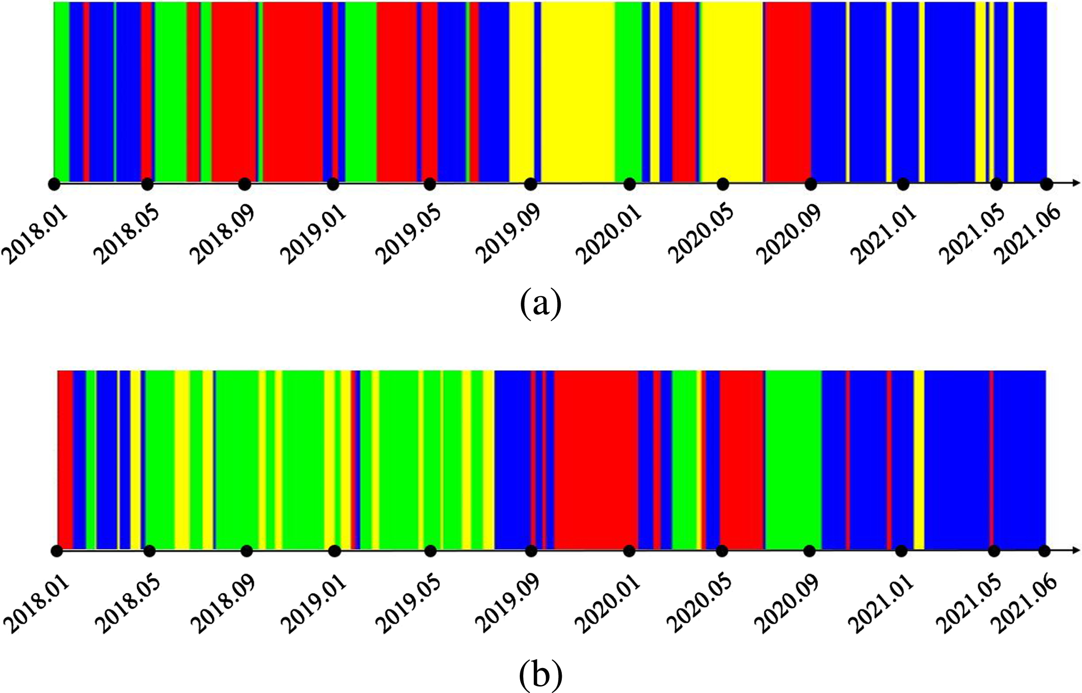
Time distribution for states on regression factors in (a) Model (4) and (b) Model (5) of call options (state 1: blue; state 2: red; state 3: yellow; state 4: green).

5 Fitting results analysis

This section employs the HMM to elaborate on the information of “hidden states” generated from the latent factors in Models (4) and (5) for both call and put options.

5.1 Fitting results on latent factors for call options

To build an HMM model, it is required to select the number of hidden states. In the experiments, the number of hidden states is determined by the Bayesian information criterion (BIC) [35]:

$BIC = - 2 \times LL + \ln (T) \times N,$ (12) where LL is the log likelihood of HMM, T is the length of sequences, and N is the number of hidden states. According to BIC, the number of hidden states N that minimizes the value of BIC is selected as the optimal one. Table 6 shows the values of BIC when the number of states ranges from 2 to 6. It can be seen that the optimal number of hidden states determined by BIC is 4 in all experiments. The hidden states grouped by the latent factors are the basis for discussing the time distribution, the characteristics, and the transition of IVS.

Table 7

The mean vector and covariance matrix of the regression factors in Model (4) under each state for call options

	$\hat{μ}$	$\hat{Σ}$
1	$[\begin{matrix} - 1.643 \\ 1.777 \\ 5.744 \\ 0.138 \\ - 4.212 \end{matrix}]$	$[\begin{matrix} 0.018 & - 0.072 & - 0.084 & - 0.319 & 0.109 \\ - 0.072 & 1.206 & - 0.148 & 0.059 & - 0.164 \\ - 0.084 & - 0.148 & 19.502 & 0.175 & - 0.027 \\ - 0.319 & 0.059 & 0.175 & 0.031 & - 0.175 \\ 0.109 & - 0.164 & - 0.027 & - 0.175 & 4.064 \end{matrix}]$
2	$[\begin{matrix} - 1.341 \\ 0.586 \\ 3.410 \\ - 0.121 \\ - 1.983 \end{matrix}]$	$[\begin{matrix} 0.023 & 0.043 & - 0.061 & - 0.216 & - 0.010 \\ 0.043 & 1.097 & - 0.174 & - 0.029 & - 0.178 \\ - 0.061 & - 0.174 & 22.086 & 0.136 & - 0.005 \\ - 0.216 & - 0.029 & 0.136 & 0.023 & - 0.047 \\ - 0.010 & - 0.178 & - 0.005 & - 0.047 & 2.780 \end{matrix}]$
3	$[\begin{matrix} - 2.008 \\ 3.969 \\ 4.001 \\ 0.352 \\ - 8.002 \end{matrix}]$	$[\begin{matrix} 0.020 & - 0.108 & - 0.091 & - 0.035 & 0.138 \\ - 0.108 & 2.226 & - 0.750 & - 0.080 & - 0.560 \\ - 0.091 & - 0.750 & 47.802 & 0.329 & 0.040 \\ - 0.035 & - 0.080 & 0.329 & 0.028 & - 0.327 \\ 0.138 & - 0.560 & 0.040 & - 0.327 & 9.332 \end{matrix}]$
4	$[\begin{matrix} - 1.807 \\ 1.063 \\ 15.544 \\ 0.330 \\ - 6.731 \end{matrix}]$	$[\begin{matrix} 0.031 & - 0.075 & - 0.101 & - 0.183 & 0.141 \\ - 0.075 & 2.981 & - 0.706 & 0.473 & - 0.743 \\ - 0.101 & - 0.706 & 83.214 & - 0.084 & - 0.132 \\ - 0.183 & 0.473 & - 0.084 & 0.100 & - 0.660 \\ 0.141 & - 0.743 & - 0.132 & - 0.660 & 20.134 \end{matrix}]$

Table 8

The mean vector and covariance matrix of the regression factors in Model (5) under each state for call options

	$\hat{μ}$	$\hat{Σ}$
1	$[\begin{matrix} - 0.320 \\ 0.265 \\ - 2.252 \\ 0.335 \\ - 0.309 \\ 0.076 \end{matrix}]$	$[\begin{matrix} 0.353 & - 0.036 & - 0.016 & - 0.457 & 0.318 & 0.046 \\ - 0.036 & 0.450 & - 0.198 & - 0.262 & 0.287 & - 0.237 \\ - 0.016 & - 0.198 & 0.329 & 0.061 & - 0.001 & - 0.021 \\ - 0.457 & - 0.262 & 0.061 & 1.341 & - 1.240 & 0.204 \\ 0.318 & 0.287 & - 0.001 & - 1.240 & 1.164 & - 0.289 \\ 0.046 & - 0.237 & - 0.021 & 0.204 & - 0.289 & 0.345 \end{matrix}]$
2	$[\begin{matrix} - 1.280 \\ 1.112 \\ 0.266 \\ - 0.266 \\ 0.733 \\ - 1.273 \end{matrix}]$	$[\begin{matrix} 0.217 & - 0.125 & 0.074 & - 0.095 & 0.154 & - 0.026 \\ - 0.125 & 1.018 & - 0.916 & - 0.188 & 0.145 & - 0.337 \\ 0.074 & - 0.916 & 1.868 & - 0.095 & 0.300 & - 0.103 \\ - 0.095 & - 0.188 & - 0.095 & 0.788 & - 0.831 & 0.349 \\ 0.154 & 0.145 & 0.300 & - 0.831 & 1.222 & - 0.621 \\ - 0.026 & - 0.337 & - 0.103 & 0.349 & - 0.621 & 0.812 \end{matrix}]$
3	$[\begin{matrix} 0.336 \\ - 0.426 \\ 0.939 \\ - 0.176 \\ 0.395 \\ - 0.487 \end{matrix}]$	$[\begin{matrix} 0.336 & - 0.126 & - 0.151 & - 0.476 & 0.376 & 0.138 \\ - 0.126 & 0.876 & - 0.736 & 0.185 & 0.075 & - 0.711 \\ - 0.151 & - 0.736 & 1.684 & 0.011 & - 0.058 & 0.022 \\ - 0.476 & 0.185 & 0.011 & 0.999 & - 0.784 & - 0.120 \\ 0.376 & 0.075 & - 0.058 & - 0.784 & 0.765 & - 0.218 \\ 0.138 & - 0.711 & 0.022 & - 0.120 & - 0.218 & 0.994 \end{matrix}]$
4	$[\begin{matrix} 0.897 \\ - 0.715 \\ - 0.237 \\ - 0.167 \\ - 0.217 \\ 0.790 \end{matrix}]$	$[\begin{matrix} 0.542 & 0.033 & - 0.035 & - 0.2571 & 0.157 & - 0.010 \\ 0.033 & 0.330 & - 0.101 & - 0.132 & 0.123 & - 0.188 \\ - 0.035 & - 0.101 & 0.508 & 0.072 & - 0.030 & - 0.023 \\ - 0.257 & - 0.132 & 0.072 & 0.591 & - 0.367 & 0.074 \\ 0.157 & 0.123 & - 0.020 & - 0.367 & 0.327 & - 0.106 \\ - 0.010 & - 0.188 & - 0.023 & 0.074 & - 0.106 & 0.235 \end{matrix}]$

For Shanghai 50ETF call options, according to the regression factors in Models (4) and (5), the obtained states of daily IVS are presented in Fig. 3, where the corresponding optimal values of the mean vector and covariance matrix given by the Baum-Welch algorithm are presented in Tables 7 and 8. As shown in Fig. 3 and Tables 7 and 8, it can be observed as follows:

For state 1 in Models (4) and (5), the implied volatilities are significantly positively affected by the curvature of moneyness, which exist at the beginning of 2018 and almost the first half of 2021. The existence may be caused by the adjustment to the strike price and the fluctuation of the RMB exchange rate against the dollar, respectively.

The second half of 2018 is mainly occupied by state 2 in Model (4) and state 4 in Model (5). For these two states, the maturity and moneyness have slight effects on the implied volatility. Consequently, the implied volatilities in this period are more stable than those in other periods. Especially, state 2 in Model (4) is the only state where the implied volatility is negatively correlated with maturity.

For state 3 in Model (4) and state 2 in Model (5), the impacts of the slope and curvature of moneyness on the implied volatilities are similar, and the interaction of moneyness and maturity has a large negative effect on the implied volatilities. These two states appear frequently during the period from late 2019 to the first half of 2021, possibly due to the impact of COVID-19 on the global economy.

For state 4 in Model (4) and state 3 in Model (5), the implied volatility is significantly affected by the positive effect from the curvature of moneyness. In addition, state 3 in Model (5) covers almost every month from the second half of 2018 to the first half of 2019, but no existence in 2020.

In the constructed HMM, the initial state distributions for Models (4) and (5) of call options are ${\hat{π}}_{1} = [0.381, 0.277, 0.209, 0.133]^{T}$ and ${\hat{π}}_{2} = [0.356, 0.180, 0.129, 0.335]^{T}$ , and the obtained state transition probability matrices $\hat{A} = [a_{ij}]$ with a_ij representing the probability of transition from the state q_i to the state q_j for Models (4) and (5) are as follows:

$\begin{matrix} {\hat{A}}_{1} = [\begin{matrix} 0.931 & 0.017 & 0.028 & 0.015 \\ 0.048 & 0.952 & 4.902 E - 62 & 7.357 E - 15 \\ 0.049 & 1.908 E - 31 & 0.944 & 0.007 \\ 0.028 & 0.051 & 0.010 & 0.912 \end{matrix}], \\ {\hat{A}}_{2} = [\begin{matrix} 0.942 & 0.028 & 0.009 & 0.021 \\ 0.074 & 0.926 & 3.051 E - 34 & 3.757 E - 24 \\ 0.055 & 0.018 & 0.850 & 0.077 \\ 0.004 & 3.131 E - 34 & 0.048 & 0.948 \end{matrix}] . \end{matrix}$

From these two matrices, the probability of each state maintaining its own state is much larger than the transition to others, among which the state whose implied volatilities are affected slightly by the maturity and moneyness (state 2 in Model (4) and state 4 in Model (5)) has the largest probability to stay its own state. The state whose implied volatilities are significantly affected by the positive effect from the curvature of moneyness (state 4 in Model (4) and state 3 in Model (5)) is easy to transfer to the state whose implied volatilities are affected slightly by the maturity and moneyness (state 2 in Model (4) and state 4 in Model (5)).

In addition, some differences exist in the transition matrices for Models (4) and (5):

In Model (4), the state whose implied volatilities are affected slightly by the maturity and moneyness (state 2), and the state whose implied volatilities are deeply affected by the interaction of moneyness and maturity (state 3) most probably only transfer to the state whose implied volatilities are all most positively affected by the curvature of moneyness (state 1).

In Model (5), the state whose implied volatilities are deeply affected by the interaction of moneyness and maturity (state 2) is highly unlikely to be transferred from the state whose implied volatilities are affected slightly by the maturity and moneyness (state 4), but highly possible to only transition to the state whose implied volatilities are all most positively affected by the curvature of moneyness (state 1).

5.2 Fitting results on latent factors for put options

In a similar manner, for Models (4) and (5), the obtained state distributions of daily IVS are shown in Fig. 4, and the corresponding statistical distributions of the regression factors in each state are shown in Tables 9 and 10. In addition, the initial state distributions are ${\hat{π}}_{3} = [0.317, 0.306, 0.107, 0.270]^{T}$ and ${\hat{π}}_{4} = [0.275, 0.384, 0.108, 0.233]^{T}$ , and the transition matrices between hidden states are:

$\begin{matrix} {\hat{A}}_{3} = [\begin{matrix} 0.954 & 0.033 & 0.004 & 0.010 \\ 0.052 & 0.901 & 0.008 & 0.040 \\ 4.806 E - 21 & 0.044 & 0.956 & 3.746 E - 17 \\ 1.832 E - 13 & 0.056 & 1.385 E - 34 & 0.944 \end{matrix}], \\ {\hat{A}}_{4} = [\begin{matrix} 0.918 & 0.074 & 0.004 & 0.004 \\ 0.052 & 0.893 & 0.003 & 0.051 \\ 1.37 E - 10 & 0.044 & 0.956 & 3.514 E - 08 \\ 0.011 & 0.065 & 0.005 & 0.919 \end{matrix}], \end{matrix}$ where ${\hat{A}}_{3}$ and ${\hat{A}}_{4}$ are the state transition matrices for Models (4) and (5), respectively.

Fig. 4

Time distribution for states on regression factors in (a) Model (4) and (b) Model (5) of put options (state 1: blue; state 2: red; state 3: yellow; state 4: green).

Table 9

The mean vector and covariance matrix of the regression factors in Model (4) under each state for put options

	$\hat{μ}$	$\hat{Σ}$
1	$[\begin{matrix} - 1.717 \\ - 1.676 \\ 9.280 \\ 0.636 \\ 7.388 \end{matrix}]$	$[\begin{matrix} 0.014 & 0.218 & 0.039 & - 0.117 & - 0.143 \\ 0.218 & 1.547 & 0.368 & - 0.084 & - 0.442 \\ 0.039 & 0.368 & 32.561 & 0.145 & 0.238 \\ - 0.117 & - 0.084 & 0.145 & 0.050 & 0.272 \\ - 0.143 & - 0.442 & 0.238 & 0.272 & 7.790 \end{matrix}]$
2	$[\begin{matrix} - 1.533 \\ - 0.955 \\ 6.870 \\ 0.157 \\ 4.022 \end{matrix}]$	$[\begin{matrix} 0.022 & 0.029 & - 0.045 & - 0.051 & 0.030 \\ 0.029 & 0.606 & 0.134 & 0.074 & - 0.141 \\ - 0.045 & 0.134 & 8.802 & 0.064 & 0.018 \\ - 0.051 & 0.074 & 0.064 & 0.027 & 0.018 \\ 0.030 & - 0.141 & 0.018 & 0.018 & 2.065 \end{matrix}]$
3	$[\begin{matrix} - 2.091 \\ - 2.879 \\ 11.733 \\ 0.584 \\ 10.363 \end{matrix}]$	$[\begin{matrix} 0.022 & 0.601 & 0.297 & - 0.187 & - 0.285 \\ 0.601 & 5.294 & 2.162 & - 0.401 & - 1.396 \\ 0.297 & 2.162 & 109.116 & - 0.102 & - 0.448 \\ - 0.187 & - 0.401 & - 0.102 & 0.041 & 0.338 \\ - 0.285 & - 1.396 & - 0.448 & 0.338 & 13.898 \end{matrix}]$
4	$[\begin{matrix} - 1.330 \\ - 0.514 \\ 3.038 \\ - 0.123 \\ 1.671 \end{matrix}]$	$[\begin{matrix} 0.027 & 0.011 & - 0.038 & - 0.247 & - 0.003 \\ 0.011 & 0.370 & 0.103 & - 0.021 & - 0.098 \\ - 0.038 & 0.103 & 13.275 & 0.096 & 0.086 \\ - 0.247 & - 0.021 & 0.096 & 0.040 & 0.067 \\ - 0.003 & - 0.098 & 0.086 & 0.067 & 1.831 \end{matrix}]$

In contrast with call options, the interaction from maturity and moneyness has a much larger impact on the IVS of put options. The states in put options with the same state number from Models (4) and (5) have similarities in distribution and transition:

The state whose implied volatilities are slightly affected by the slope and curvature of maturity (state 2) has the smallest probability to maintain itself. From the first half of 2018 to the first half of 2019, and from July 2020 to September 2020, it is easy to transfer to and from the state whose implied volatilities are slightly affected by the slope of maturity and moneyness (state 4), which indicates the existence of the slight fluctuation during this period. From May 2019 to August 2019, and from September 2020 to June 2020, it is easy to transfer to the state whose implied volatilities are more affected by maturity than others (state 1), which indicates maturity has a strong impact on the implied volatility during this period.

The state that the implied volatilities are deeply affected by maturity and moneyness, especially the curvature in the dimension of moneyness (state 3), has the largest probability to maintain itself, which occurs in January 2018, and from October 2019 to January 2020. This may be due to the release of new rules in strikes for the Shanghai 50ETF options at the beginning of 2018 and the emergence of COVID-19 at the end of 2019. Beyond that, it only transfers to the state whose IVS is slightly affected by maturity (state 2).

Table 10

The mean vector and covariance matrix of the regression factors in Model (5) under each state for put options

	$\hat{μ}$	$\hat{Σ}$
1	$[\begin{matrix} - 0.463 \\ - 0.334 \\ 0.325 \\ 0.801 \\ - 0.366 \\ 0.650 \end{matrix}]$	$[\begin{matrix} 0.205 & 0.207 & 0.077 & - 0.055 & - 0.005 & - 0.104 \\ 0.207 & 0.968 & 0.416 & 0.384 & - 0.528 & - 0.505 \\ 0.077 & 0.416 & 1.108 & - 0.077 & 0.205 & 0.306 \\ - 0.055 & 0.384 & - 0.077 & 0.647 & - 0.682 & - 0.284 \\ - 0.005 & - 0.528 & 0.205 & - 0.682 & 0.881 & 0.538 \\ - 0.104 & - 0.505 & 0.306 & - 0.284 & 0.538 & 0.679 \end{matrix}]$
2	$[\begin{matrix} 0.265 \\ 0.531 \\ - 0.320 \\ 0.141 \\ - 0.396 \\ - 0.666 \end{matrix}]$	$[\begin{matrix} 0.551 & 0.113 & - 0.223 & - 0.325 & 0.141 & - 0.193 \\ 0.113 & 0.187 & 0.067 & - 0.054 & 0.002 & - 0.103 \\ - 0.223 & 0.067 & 0.402 & 0.180 & - 0.044 & 0.168 \\ - 0.325 & - 0.054 & 0.180 & 0.313 & - 0.149 & 0.157 \\ 0.141 & 0.002 & - 0.044 & - 0.149 & 0.124 & - 0.019 \\ - 0.193 & - 0.103 & 0.168 & 0.157 & - 0.019 & 0.215 \end{matrix}]$
3	$[\begin{matrix} - 1.656 \\ - 1.150 \\ 0.872 \\ - 0.251 \\ 0.854 \\ 1.441 \end{matrix}]$	$[\begin{matrix} 0.460 & 0.503 & 0.326 & - 0.636 & 0.693 & - 0.167 \\ 0.503 & 2.857 & 1.925 & 0.438 & - 0.874 & - 1.503 \\ 0.326 & 1.925 & 2.786 & - 0.256 & 0.2582 & - 0.336 \\ - 0.636 & 0.438 & - 0.256 & 1.982 & - 2.434 & - 0.617 \\ 0.693 & - 0.874 & 0.258 & - 2.434 & 3.192 & 1.103 \\ - 0.167 & - 1.503 & - 0.336 & - 0.617 & 1.103 & 1.261 \end{matrix}]$
4	$[\begin{matrix} 0.822 \\ 0.064 \\ - 0.251 \\ - 0.973 \\ 0.620 \\ - 0.331 \end{matrix}]$	$[\begin{matrix} 0.603 & 0.245 & - 0.133 & - 0.194 & 0.033 & - 0.204 \\ 0.245 & 0.364 & 0.014 & - 0.043 & - 0.071 & - 0.252 \\ - 0.133 & 0.014 & 0.380 & 0.108 & - 0.027 & 0.176 \\ - 0.194 & - 0.043 & 0.108 & 0.324 & - 0.307 & 0.060 \\ 0.033 & - 0.071 & - 0.027 & - 0.307 & 0.447 & 0.094 \\ - 0.204 & - 0.252 & 0.176 & 0.060 & 0.094 & 0.316 \end{matrix}]$

Table 11

The evaluation of predictive ability

	Model	RMSE	MAE	MAPE(%)
Call options	ARIMA(1,0,1) with Model (4)	0.159	0.154	9.650
	ARIMA(1,0,1) with Model (5)	0.141	0.136	8.574
	VAR(1) with Model (4)	0.138	0.131	8.291
	VAR(1) with Model (5)	0.134	0.127	7.978
	SVR with Model (4)	0.111±0.035	0.093±0.027	6.354±0.020
	SVR with Model (5)	0.094±0.044	0.087±0.038	5.864±0.026
	HMM with Model (4)	0.104±0.049	0.088±0.042	5.871±0.030
	HMM with Model (5)	0.098±0.041	0.085±0.037	5.604±0.026
Put options	ARIMA(1,0,1) with Model (4)	0.132	0.121	7.358
	ARIMA(1,0,1) with Model (5)	0.117	0.105	6.427
	VAR(1) with Model (4)	0.113	0.101	6.247
	VAR(1) with Model (5)	0.112	0.101	6.201
	SVR with Model (4)	0.100±0.032	0.089±0.031	5.526±0.020
	SVR with Model (5)	0.098±0.040	0.087±0.041	5.442±0.024
	HMM with Model (4)	0.097±0.037	0.084±0.036	5.261±0.021
	HMM with Model (5)	0.095±0.048	0.082±0.050	5.087±0.028

6 Out-of-sample forecasting

This section further examines the performance of HMMs for the implied volatility prediction. The sample set is divided into training data and testing data. The total length of the time series is 846 in call options and 847 in put options, where the data from January 2, 2018, to May 31, 2021, are treated as the training set, and the remaining data in the last month, i.e., from June 1, 2021, to June 30, 2021, are treated as the testing set.

With the state sequence obtained in Section 5, we can calculate the latent factors utilized in Models (4) and (5) by predicting the states, which can further realize the forecast of implied volatility. Following this process, the prediction results of the latent factors and implied volatility are obtained, and meanwhile, the corresponding states to describe the characteristics of the predicted IVS are also achieved. In the following experiments, the criteria used to test the accuracy of prediction include Root Mean Squared Error (RMSE), Mean Absolute Error (MAE), and Mean Absolute Percentage Error (MAPE) (given in percentage): $RMSE = \sqrt{\frac{1}{L} \sum_{t = 1}^{L} (σ_{t}^{IV} - {\hat{σ}}_{t}^{IV})^{2}},$ (13) $MAE = \frac{1}{L} \sum_{t = 1}^{L} | σ_{t}^{IV} - {\hat{σ}}_{t}^{IV} |,$ (14) $MAPE = \frac{1}{L} \sum_{t = 1}^{L} | \frac{σ_{t}^{IV} - {\hat{σ}}_{t}^{IV}}{σ_{t}^{IV}} | \times 100 %,$ (15) where $σ_{t}^{IV}$ and ${\hat{σ}}_{t}^{IV}$ are the implied volatility and the predicted implied volatility at time t, and L is the length of the prediction set.

For the comparison purpose, the autoregressive integrated moving average (ARIMA) model, the vector auto-regression (VAR) model, and the support vector regression (SVR) model are adopted to be our benchmarks. Table 11 shows the results of RMSE, MAE, and MAPE of ARIMAs, VARs, SVRs, and HMMs, where the corresponding values of mean value and standard deviation for SVRs and HMMs are also presented. We can observe that the HMM has a better predictive capability than other models in the prediction of implied volatilities.

7 Conclusion

In this study, we employ the regime-switching framework of the hidden Markov model (HMM) to model the latent states of the Shanghai 50ETF options. First, we fit the cross-sectional models (4) and (5) for implied volatility surface (IVS), and the regression factors estimated by OLS are treated as the reference of IVS. Then, the HMM is built to analyze the estimated coefficients to further extract the characteristics, the time-dependent structure, and the transition mechanism existing in the IVS. The empirical results indicate that the latent factors of IVS are successfully captured, and the achieved structure reflects different financial characteristics, where some of their typical features and transition are associated with certain events. In addition, the HMM performs better in the implied volatility prediction compared with other benchmark prediction models.

The proxies of IVS used in this study are the latent factors incorporating the impact of option maturity and moneyness. Some other factors, such as dividends, exchange rates, and liquidity costs could be considered in future research. In addition, the first-order HMM used in this study could be extended to second-order or even higher-order models in future works.

References

Brüggemann

, Härdle

, Mungo

and Trenkler

, Varmodeling for dynamic loadings driving volatility strings, Journal of Financial Econometrics 6(3) (2008), 361–381.

Georgios

and Tsekrekos

A.E.

, Predictable dynamics in implied volatility surfaces from OTC currency options, Journal of Banking & Finance 34(6) (2010), 1175–1188.

Harvey

C.R.

and Whaley

R.E.

, Market volatility prediction and the efficiency of the S&P 100 index option market, Journal of Financial Economics 31(1) (1992), 43–73.

Bernales

and Guidolin

, Can we forecast the implied volatility surface dynamics of equity options? Predictability and economic value tests, Journal of Banking & Finance 46 (2014), 326–342.

Konstantinidi

, Skiadopoulos

and Tzagkaraki

, Can the evolution of implied volatility be forecasted? Evidence from European and US implied volatility indices, Journal of Banking & Finance 32(11) (2008), 2401–2411.

Chalamandaris

and Tsekrekos

A.E.

, How important is the term structure in implied volatility surface modeling? Evidence from foreign exchange options, Journal of International Money and Finance 30(4) (2011), 623–640.

Chen

, Zhou

and Li

, An efficient estimate and forecast ofthe implied volatility surface: A nonlinear Kalman filter approach, Economic Modelling 58 (2016), 655–664.

Dumas

, Fleming

and Whaley

R.E.

, Implied volatility functions: Empirical tests, The Journal of Finance 53(6) (1998), 2059–2106.

Cont

and Da

, Fonseca, Dynamics of implied volatility surfaces, Quantitative Finance 2(1) (2002), 45.

10.

Goncalves

and Guidolin

, Predictable dynamics in the S&P 500 index options implied volatility surface, The Journal of Business 79(3) (2006), 1591–1635.

11.

Ignacio

, Gonzalo

and Gregorio

, Why do we smile? On the determinants of the implied volatility function, Journal of Banking & Finance 23(8) (1999), 1151–1179.

12.

Skiadopoulos

, Hodges

and Clewlow

, The dynamics of the S&P 500 implied volatility surface, Review of Derivatives Research 3(3) (2000), 263–282.

13.

Fengler

M.R.

, Härdle

W.K.

and Villa

, The dynamics of impliedvolatilities: A common principal components approach, Review ofDerivatives Research 6(3) (2003), 179–202.

14.

Fengler

M.R.

, Härdle

W.K.

and Mammen

, A semiparametric factor model for implied volatility surface dynamics, Journal of Financial Econometrics 5(2) (2007), 189–218.

15.

Christoffersen

, Heston

and Jacobs

, The shape and term structure of the index option smirk: Why multifactor stochastic volatility models work so well, Management Science 55(12) (2009), 1914–1932.

16.

Takahiro

, Yu

, Takamitsu

and Naoki

, Modelling state-transition dynamics in resting-state brain signals by the hidden markov and gaussian mixture models, European Journal of Neuroscience 54(4) (2021), 5404–5416.

17.

Korayem

M.H.

, Azargoshasb

, Korayem

A.H.

and Tabibian

, Design and implementation of the voice command recognition and the sound source localization system for humanrobot interaction, Robotica 39(10) (2021), 1779–1790.

18.

Park

S.-H.

, Lee

J.-H.

, Song

J.-W.

and Park

T.-S.

, Forecasting changedirections for financial time series using hidden markov model, in, Rough Sets and Knowledge Technology, proceedings 5589(2009), 184–191.

19.

S.-T.

and Cheng

Y.-C.

, A hidden Markov model-based forecasting model for fuzzy time series, WSEAS Transactions on Systems 5(8) (2006), 1919–1924.

20.

Dueker

and Neely

C.J.

, Can Markov switching models predict excess foreign exchange returns? Journal of Banking & Finance 31(2) (2007), 279–296.

21.

Dias

J.G.

, Vermunt

J.K.

, Ramos

Mixture hidden Markov models in finance research, in Advances in data analysis, data handling and business intelligence (2009), 451–459, Springer.

22.

Geweke

and Amisano

, Hierarchical Markov normal mixture modelswith applications to financial asset returns, Journal ofApplied Econometrics 26(1) (2011), 1–29.

23.

Oelschläger

, Adam

Detecting bearish and bullish markets in financial time series using hierarchical hidden Markov models, Statistical Modelling (2021), p. https://doi.org/10.1177/1471082X211034048.

24.

Werge

, Predicting risk-adjusted returns using an asset independent regime-switching model, Expert Systems with Applications 184 (2021), 115576.

25.

Zhang

, Jiang

, Fang

, Zeng

and Xu

, High-order HiddenMarkov Model for trend prediction in financial time series, Physica A: Statistical Mechanics and its Applications 517 (2019), 1–12.

26.

Somani

, Talele

, Sawant

Stock market prediction using Hidden Markov Model, in 2014 IEEE 7th joint international information technology and 651 artificial intelligence conference (2014), 89–92, IEEE.

27.

Black

and Scholes

, The pricing of options and corporateliabilities, Journal of Political Economy 81(3) (1973), 637–654.

28.

Poon

S.H.

and Granger

C.W.

, Forecasting volatility in financial markets: A review, Journal of Economic Literature 41(2) (2003), 478–539.

29.

Wang

, Chen

, Tao

and Zhang

, Modelling the impliedvolatility surface based on shanghai 50ETF options, EconomicModelling 64 (2017), 295–301.

30.

Rabiner

L.R.

, A tutorial on hidden Markov models and selectedapplications in speech recognition, Proceedings of the IEEE 77(2) (1989), 257–286.

31.

Liporace

, Maximum likelihood estimation for multivariateobservations of Markov sources, IEEE Transactions onInformation Theory 28(5) (1982), 729–734.

32.

Juang

B.-H.

, Maximum-likelihood estimation for mixture multivariate stochastic observations of Markov chains, AT&T Technical Journal 64(6) (1985), 1235–1249.

33.

Juang

B.-H.

, Levinson

and Sondhi

, Maximum likelihood estimation for multivariate mixture observations of markov chains (corresp.), IEEE Transactions on Information Theory 32(2) (1986), 307–309.

34.

Sui

, Lung

and Yang

, Predictable Dynamics in the Implied Volatility Surface Based on Weighted Least Squares: Evidence from Soybean Meal Futures Options in China, Emerging Markets Finance and Trade 56(11) (2020), 2625–2638.

35.

Schwarz

Estimating the dimension of a model, The Annals of Statistics (1978), 461–464.

Hidden Markov model-based modeling and prediction for implied volatility surface 1

Abstract

Keywords

1 Introduction

2 Related Work

Table 1 Basic notations used in this study

3.1 The definition of implied volatility surface

4.1 Data selection and filtering

4.2 Statistical analysis of implied volatility surface

5.1 Fitting results on latent factors for call options

References

Table 1
Basic notations used in this study