A novel stacking framework with PSO optimized SVM for effective disease classification

Abstract

Disease diagnosis is very important in the medical field. It is essential to diagnose chronic diseases such as diabetes, heart disease, cancer, and kidney diseases in the early stage. In recent times, ensembled-based approaches giving effective predictive performance than individual classifiers and gained attention in assisting doctors with early diagnosis. But one of the challenges in these approaches is dealing with class-imbalanced data and improper configuration of ensemble classifiers with optimized parameters. In this paper, a novel 3-level stacking approach with ADASYN oversampling technique with PSO Optimized SVM meta-model (Stacked-ADASYN-PSO) is proposed. Our proposed Stacked-ADASYN-PSO model uses base models such as Logistic regression(LR), K-Nearest neighbor (KNN), Support Vector Machine (SVM), Decision Tree (DT), and Multi-Layer Perceptron (MLP) in layer-0. In layer-1 three meta classifiers namely LR, KNN, and Bagging DT are used. In layer-2 PSO optimized SVM used as the final meta-model to combine the previous layer predictions. To evaluate the robustness of the proposed model It is tested on five benchmark disease datasets from the UCI machine learning repository. These results are compared with state-of-the-art ensemble models and non-ensemble models. Results demonstrated that the proposed model performance is superior in terms of AUC, accuracy, specificity, and precision. We have performed statistical analysis using paired T-tests with a 95% confidence level and our proposed stacking model is significantly differs when compared to base classifiers.

Keywords

Disease diagnosis particle swarm optimization oversampling stacking class imbalance ensemble

1 Introduction

Disease diagnosis is a process by which a doctor determines whether a patient has a disease based on the patient’s health condition and to determine the type of disease the patient has. In an actual disease diagnosis environment especially when there is a huge number of patients and the amount of data to be processed is too large, it may be troublesome for doctors to handle in a short period. In disease diagnosis to improve the predictive performance, we ensure that data should be preprocessed and processed with outliers, missing values, and data scaling. Various preprocessing techniques such as Inter Quartile Range (IQR) are used to assess the variability where most of your values lie. Most of the disease datasets are class-imbalanced, and classification results are biased towards the majority class. There is much attention to dealing with class imbalanced data for effective disease diagnosis. In the literature, there are various oversampling techniques are already used in disease diagnosis such as Synthetic Minority Over-Sampling Technique (SMOTE), Borderline Synthetic Minority Over-Sampling Technique (BSMOTE), Adaptive Synthetic Minority Over-Sampling Technique (ADASYN), Random Over-sampling Technique (ROS) [1]. SMOTE creates new artificial instances utilizing knowledge about the neighbors that surround each sample of the minority class [2]. Whereas in other approaches oversampled instances are arbitrarily chosen through duplication. To determine the k closest neighbors of a given minority data instance from the neighborhood, SMOTE uses the K-Nearest Neighbour (K-NN) technique. BSMOTE steps are similar to SMOTE to produce artificial data [3]. In order to solve the issue of minority instance misclassification (and to improve the detection rate of minority instances), it also reinforces the border by taking borderline minority class instances into account while producing synthetic data.ADASYN creates more minority samples near the decision border, helping to develop the classification boundary [4]. Based on the percentage of majority samples in the KNN sets of the minority class, this technique will calculate the number of synthesized minority samples.ROS replicates minority class instances and inserts them into the same class to provide a balanced training dataset, which is the oldest oversampling technique [5].

Various ensembled-based approaches have already been used to improve the predictive performance of models such as bagging [6], boosting, and stacking [7]. In bagging [6] bootstrapped approach is used for homogeneous classifiers to maintain diversity and reduce bias. Boosting [8] is an ensemble modeling technique that attempts to build a strong classifier from the pool of weak classifiers. It is done by building a model by using weak models in series. While bagging and boosting used homogeneous weak learners for ensemble, stacking often considers heterogeneous weak learners, learns them in parallel, and combines them by training a meta-learner to output a prediction based on the different weak learner’s predictions [9].

Hyper-parameter optimization will improve the predictive performance of the individual classifier [10]. In the literature, various search techniques are used for hyperparameter optimization such as grid search, random search, etc [11]. In the stacked ensemble parameter optimization of the base model as well as the meta-model is also important otherwise, it may impact the performance of the ensemble model [10]. Various meta-heuristic algorithms such as evolutionary-based, nature-inspired algorithms are used for hyperparameter optimization [12]. Particle swarm optimization (PSO) is an algorithm for swarm intelligence based on stochastic and population-based adaptive optimization inspired by the social behavior of bird flocks and fish swarms [13].

The best configuration of the stacking model will give an effective predictive performance. so selecting optimal base models and meta-models are important in the stacking approach [14].

Following is the arrangement of the remaining sections. A literature review is in the second section, and the Background of the proposed work is in the third section. The proposed work is covered in Section 4, results are covered in Section 5, and the Discussion is in Section 5 followed by a conclusion.

1.1 Motivation

In disease diagnosis, most of the datasets are class imbalanced. ML models are biased toward the majority of samples in class imbalanced data. To address this problem various oversampling approaches are used. Directly applying oversampling techniques does not guarantee the improvement of performance due to noise while generating synthetic data. To overcome this we combined oversampling and ensemble learning to improve the predictive performance. But in the ensemble approach, most of the researchers attempted the optimization of base classifiers with limited research on the optimization of meta-classifiers.In the stacking approach if we are increasing the number of layers there should be an effective meta-model that can combine the predictions of the previous layers. we have optimized base classifiers with grid search and the last level meta-model with Particle swarm optimization(PSO) with a novel fitness function. Research questions are to be addressed with the proposed approach.

RQ 1. Can we improve predictive performance with oversampling and ensemble approach?

RQ 2. Extended stacking approach(Multi-level) is better in prediction than the basic stacking approach?

RQ 3. Does final Meta-model parameter optimization make any improvement in overall performance?

RQ 4. How does the proposed model have more significance than other base-level models statistically?

1.2 Contributions

The following contributions are made to improve the performance.

Various oversampling techniques such as SMOTE, BSMOTE, ADASYN, and ROS used for class imbalance and chosen suitable oversampling techniques for the proposed model.

Optimized parameters of base classifiers and level 1 meta-model parameters with grid search and level-2 meta-model parameters with Particle swarm Optimization(PSO).

Proposed hybrid model consists of ADASYN oversampling and a 3-level stacking approach with a PSO-optimized SVM meta-model.

Finally, statistical analysis with paired T-test was performed to test the significance of the proposed model with base-level classifiers.

2 Literature review

Kalagotla et al. proposed a novel stacking technique on PID and compared the AdaBoost and stacking revealing that the accuracy of stacking a heterogeneous ensemble 78.2% outperforms the AdaBoost a homogeneous ensemble 76.54% [15]. D. Joshi et al. used the R tool on the PID dataset to predict T2DM. They applied DT and LR classifiers on PID and reported 78.26% and 74.48% accuracies respectively [16].

S. Arukonda et al. [17] proposed a disease diagnosis ensemble model. This study used four diversity-based classifiers on five data bags and optimized classifiers from a pool of 20 diverse learners using GA. This study used PID, SHD, CKD, and WBC disease datasets used to test the robustness of the models. Accuracies are 90.91%, 96.05%, 97.56%, and 98.08% respective to PID, CKD, SHD, and WBC datasets.

Singh et al.proposed a stacking approach on PID and evaluated the predictive performance of various ensemble approaches such as Bagging (L-SVM), Bagging (RBF-SVM), Bagging (Poly-SVM), Bagging (REP), Bagging (4.5), Ada boost(DS), Ada boost (C4.5), Random Subspace Method (RSM), Random Forest, Majority Voting (MV), Stacking, Stacking (LR), Stacking (NSGA-II) the proposed system achieve the highest accuracy of 83.8%, the sensitivity of 96.1%, specificity of 79.9%, f-measure of 88.5% and area under ROC curve of 85.9% [18].

S.Arkonda et al. proposed a model for Lung cancer is one of the most common cancer-related disorders with a high mortality rate, which is mostly owing to the late detection of malignancy [19].

Mohapatra et al. proposed a two-level stacking approach for detecting heart irregularities and predicting Cardiovascular disease and pre-processed with outlier detection and the stacking of classifiers for predicting heart diseases [20]. In this study, various classifiers were used to take advantage of their differences in strengths. Using MLP as the meta-learner, Obtained results with 92% accuracy. The proposed stacked classifier outperformed the traditional machine learning classifiers better in terms of overall parameter comparison with a precision of 92.6%, a sensitivity of 92.6%, and a specificity of 91%.

Sampath et al. proposed a model for cancer disease. Cancer is still a fatal illness with numerous subtypes, posing numerous hurdles in biomedical research [21].

Tiwari et al. proposed an Ensemble framework for cardiovascular disease prediction proposed framework consist of Stacking Based Ensemble learning which adds diversity to the classifier experimented on IEEE Data Port proposed stacked ensemble attained an accuracy of 92.34% [9]. Obaidat et al. proposed a stacking ensemble model for predicting heart attacks and combines a group of three base-level classifiers such as Naive Bayes, Random Forest, and Extreme Gradient Boosting (XGBoost) in the predictive model [22].

3 Background

3.1 Classifier combination for ensembles

The selection of classifiers and a combination of those for the best ensemble is a very tedious task [23]. Researchers and data analysts use various machine learning algorithms and choose the best algorithm according to the performance measures [24]. To make the best predictions, a single algorithm may be unable to capture the entire underlying structure of the data [25]. This is where the successful integration of numerous models gathered into a single meta-model has been discovered [25]. Bagging creates numerous versions of predictors and aggregates them by voting on each version and taking the average of them [6]. Bagging meta-estimator and random forest are two algorithms that use the bagging approach [6]. Boosting works similarly to bagging in that it combines numerous low-performing base learners in an adaptive manner [8]. Bagging is beneficial for data sets with noisy values, according to experimental results. Stacking is the third approach. It uses the output of selected classifiers on the training data to predict response values using another learning algorithm. The stacking generalization architecture typically consists of two layers. First, in layer 0, there is base classification, which uses basic classifiers to build the ensemble by training the dataset. It generates the second layer’s input. Second, in layer 1, the meta-classification integrates the outputs of layer 3 using a meta-classifier to build the final predictive model.

3.2 Hyperparameter optimization of classifiers

Best hyperparameters will give a better performance so optimization of hyperparameters is a very crucial step in machine learning [26]. Hyperparameter optimization is the process of selecting the right parameter values for classifiers in order to build the best prediction model. For optimizing hyperparameters, there are numerous methods available [10], including (1) grid search, (2) random search, (3) simulated annealing algorithm, (4) bayesian optimization, (5) genetic algorithm, and (6) particle swarm optimization. Grid search, random research, and Bayesian optimization are the most prevalent hyperparameter optimization methodologies [26].

The Grid search is the most basic way. For each possible combination of all hyperparameter settings, a prediction model will be built, and each model will be assessed to see which architecture produces the best results. Random search provides better models than grid search because it searches a larger, less promising configuration space. The following method, also known as the surrogate method, keeps track of previous assessment outcomes that are utilized to form a probabilistic model and converts the hyperparameters to a probability of a score on the objective function that it employs. Because they investigate the best set of hyperparameters to evaluate based on previous trials, it may be able to find a better set of hyperparameters in less time [27].

A genetic algorithm is a meta heuristic algorithm that is based on the evolutionary concept [28]. It looks for individuals that have the best chance of survival. The abilities of one generation are passed on to the next. The next generation inherits that trait from their parents and matures into better people as a result. The worst of humanity will gradually fade away. This concept will be utilized to optimize classifier hyperparameters. The population, chromosomes, and genes will be programmed to look for space, hyperparameters, and values. The fitness value will calculate and evaluate performance. On chromosomes, selection, cross-over, and mutation will be utilized to create a new generation and assess performance. These steps will be repeated until the best hyperparameters are found. Particle swarm optimization is another evolutionary optimization technique. Particle swarm optimization is less difficult to implement than the Genetic approach. It works by allowing a group of particles to move semi-randomly around the search space [13].

3.3 Outlier Removal using IQR

IQR is a data prepossessing used to remove outliers. By dividing a rank-ordered dataset into four equal portions, or quartiles, it calculates dispersion [29]. The middle values in the first and second halves of the rank-ordered dataset, respectively, are designated by the letters Q1, Q2, and Q3, while the median value for the entire set is denoted by Q2. Then, Q3-Q1 is equal to IQR. Here, data instances outside of the normal range (Q1-(1.5*IQR) or Q3+(1.5*IQR) are considered outliers.

3.4 Particle Swarm Optimization (PSO)

PSO was developed from the study of bird migration and foraging behavior by Eberhart and Kennedy near the end of the twentieth century [30]. Each member of the group has a unique perceptual capacity, which allows them to recognize the best local and global individual locations and change their next behavior accordingly. Individuals are treated as particles in a multi-dimensional search space in the method, with each particle representing a potential solution to the optimization issue. The particle characteristics are described using three factors: location, velocity, and fitness value. The fitness function determines the fitness value. The particle modifies its traveling direction and distance independently based on the ideal global fitness value, iterative arriving at the best option. we are using velocity and position updates for every iteration based on that it computes the personal best and global best and up to termination condition met or no of iterations. It takes a group of candidate solutions and uses a position-velocity updating approach to try to select the optimal one. Uses a star topology, in which each particle is drawn to the best-performing particle. The position update can be defined as: $y_{i} (t + 1) = y_{i} (t) + v_{i} (t + 1)$ (1) where y_i (t) is position value at time t v_i (t + 1 is velocity at time t+1 The velocity update rule $\begin{matrix} v_{ij} (t + 1) = w * v_{ij} (t) + c_{1} r_{1 j} (t) * [y_{ij} (t) - x_{ij} (t)] \\ + c_{2} r_{2 j} (t) * [{\hat{y}}_{j} (t) - x_{ij} (t)] \end{matrix}$ (2)

Here, c₁ and c₂ are the cognitive and social parameters respectively. They choose between two options for particle behavior: (1) pursue its own best or (2) follow the swarm’s global best position. Overall, this determines whether the swarm is explorative or exploitative. In addition, the swarm’s inertia is controlled by the parameter w.

3.5 Support Vector Machine (SVM)

SVM is a popular statistical-based supervised machine learning technique. It is used for regression and classification tasks [31]. It was developed in 1995 by Cortes and Vapnik to improve class separation and reduce prediction error. SVM is well known for working with both linear and non-linear data and is highly good at overcoming dimensionality-related problems [32]. It works well with short datasets and high-dimensional feature spaces in particular. SVM divides training samples into distinct classes when dealing with linear data by locating a hyperplane with the greatest margin. Additionally, it establishes the maximum separation between the support vectors or nearest points to the margin edge, and the hyperplane with n-1 dimensions [33]. The mathematical formula for maximizing the margin is represented by equation (1), which signifies the weight vector, the input vector, and the bias [34]. Using some kernel functions and the kernel trick, SVM uses a kernel-based approach to cope with non-linear data, locating the optimum hyperplane to linearly segregate data [35]. The list of Kernel functions that were looked through in this study to identify the best is shown below [33]. The linear kernel function is shown in equation (2), where c is a constant.

3.6 K-Nearest Neighbor (K-NN)

KNN is a non-parametric supervised machine learning technique. It was created in the early 1950s and later expanded by Thomas Cover [36]. As it uses the entire dataset to categorize the unlabeled data points by assigning them to the closest class based on the distance measurement, K-NN is regarded as a lazy learner technique. The distances that were looked for in this study to determine the best outcomes are listed below. The formulas for computing the Euclidean distance, Minkowski distance, and Manhattan distance, respectively, are represented by equations (6), (7), and (8), where k stands for the total number of neighbors and p is any real value [37]. Euclidean distance: K-NN begins by scouring the whole training dataset in search of (K) neighbors that have the shortest path between the target point and the data points. The new data is then classified using the neighborhood’s data points’ majority voting results.

3.7 Decision Tree (DT)

DT is a popular supervised machine learning approach for both classification and regression problems. Although the concept of a DT has been around since the late 1950s, it only really gained traction in 1986 when Quinlan put up the idea of trees with numerous responses [38]. It is renowned for having a structure like a tree that is simple to understand when visualized as a tree. Leaf nodes and internal nodes make up DT. The leaf nodes denote the resultant class, but the internal nodes signify a test over an attribute and have numerous branches reflecting the test outcome. The best quality features are selected using a hierarchical or statistical approach, and DT is built using a recursive divide-and-conquer strategy [39].

3.8 Multi-layer perceptron

MLP is a feed-forward network with gradient descent as a backpropagation algorithm. It reduces loss function and maximizes performance. Unlike perceptron, MLP has more than one layer. The input layer just translates the input whereas the hidden and output layer computes the weighted sum of inputs and their associated weights plus the bias of that neuron [40].

Bagging is an ensemble approach that is introduced by Breiman in 1996 [6]. It employs a bootstrapping technique to create a diverse subset of training datasets as it lessens the variance. Then, these subsets are trained parallel through multiple weak learners. Afterward, the outcome of each learner is aggregated using soft or hard voting depending on the task type.

3.9 Stacking

Stacking is another ensemble framework, where a new classifier combines a number of distinct predictions from base learners to classify the unseen sample. It was first presented by Wolpert in 1992 to completely minimize bias and variance, which increases predictive accuracy [7]. There are two layers in the stacking structure [41]. The first layer consists of many base learners, while the second layer acts like a combiner and meta-learner. Basic stacking in Fig. 1 and extended (3-level) stacking in Fig. 3 are shown.

Fig. 1

stacking ensemble model.

Fig. 2

proposed model.

Fig. 3

3-level stacking ensemble.

4 Proposed methodology

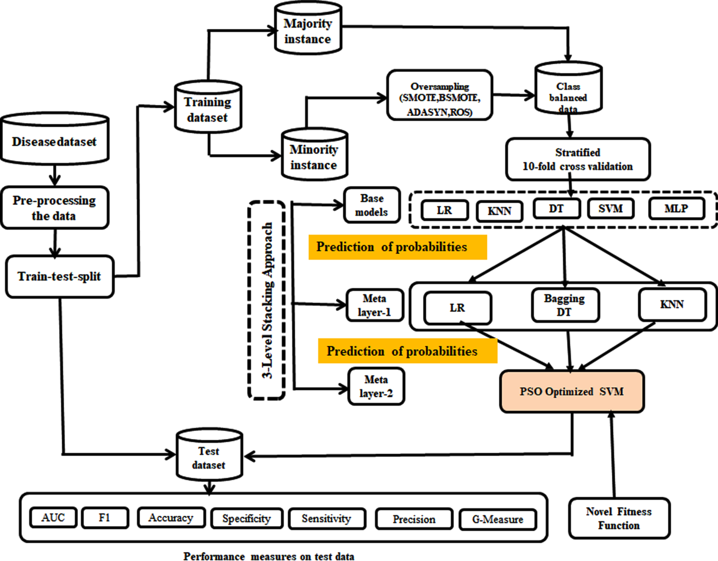
In our proposed work we have

performed preprocessing of the dataset and removed outliers, missing values, and scaled the data.

model selection using 10-FCV.

Proposed hybrid model consists of ADASYN oversampling and a 3-level stacking approach with a PSO-optimized SVM meta-model.

designed a three-layer stacking framework with KNN, DT, SVM, MLP, and LR in layer-0, Bagged DT, KNN, and LR in layer-1, and optimized SVM in layer-2.

optimized SVM hyperparameters using PSO with novel fitness function.

Finally, statistical analysis with paired T-test was performed to test the significance of the proposed model with base-level classifiers.

In proposed model is shown in Fig. 2. The 3-level proposed model is described in the section.

Initially data set will be pre-processed using IQR. Then, the dataset further experiments for best oversampling technique for class balance.

4.1 Architecture of the proposed Ensemble

An extended version of the two-layer stacking ensemble has been proposed to investigate whether stacking increases prediction model accuracy. The proposed stacked generalization is made up of three layers: (1) base classification, (2) meta classification 1, and (3) meta classification 2. To obtain the layer 2 meta-models, the proposed stacking classifier utilized five (5) base classifiers, all of which were trained using three (3) selected meta-classifiers. The three (3) meta-models formed by each meta-classifier were transmitted to the next layer, which produced the final prediction model with a single meta-classifier.

For layer 0 base classification, the proposed extended stacking classifier employs the LR, KNN, DT, SVM, and MLP algorithms. Because these ML models were chosen using 10-FCV.

Individual classifiers create prediction models with varying degrees of accuracy. Layer 0’s output prediction models were used as layer 1’s inputs.

Layer 1 meta-classifiers include LR, KNN, and bagged DT classifiers. The choice of a meta-classifier should be based on the prediction job, and as of this writing, the meta-learners have opted to produce the layer 1 output [42]. SVM was used as the proposed procedure’s layer 2 meta-classifier. The selection of distinct algorithms is motivated by the fact that they take fundamentally varied approaches to model generation and focus on data in different ways to make a meaningful contribution to ensemble implementation. On a single dataset S, different learning algorithms L₁, L₂,..., L_N are applied to examples s_k =(x_k, y_k), i.e., pairs of feature vectors (x_k) and their classifications. (y_k). The first layer generates the basis classifiers C₁, C₂,..., and C_N, where C_k = L_k. Meta-level classifiers are trained in the second layer to aggregate the outputs of base-level classifiers.

4.2 Stacking framework

A novel three-level stacking framework is proposed. In the proposed framework there are three levels.

In Level 0, LR, KNN, DT, SVM, and MLP classifiers are used.

In level 1, Bagging DT, KNN, and LR classifiers are used.

In level 2, an optimized SVM is used. Here, the SVM parameters are optimized using PSO with a novel fitness function.

4.3 Multi-level stacking appraoch

To enhance the performance of the level 2 stacking approach (level-0 base models and level-1 meta models) extended the number of levels. In our proposed model total of 3 levels (level-0 base models,level-1 meta classifiers,level-2 meta classifiers).In our proposed approach we have selected the best-performing models from a pool of ML algorithms such as LR, KNN, DT, MLP, SVM, NB, and RC. From the pool NB and RC are not selected because the cross-validation score is less. The selected models are considered base models and have undergone for stacking approach. Stacking performance may degrade if we will not do a proper configuration of ensemble classifiers. To avoid overfitting we have used 10-FCV to generate predictions of base models. All base models’ probabilistic outcomes and original class labels become auxiliary datasets for training the meta-classifiers of layer 1. In a similar way meta classifiers layer-1 will use 10-FCV and generates probabilistic outcomes here one more auxiliary dataset will generate and used for training of level-2 meta classifier. Here level-1 and level-2 depending on previous layers will predict in similar ways but level-1 and level-2 classifiers are completely different. Here selected meta classifiers used in level-1 are LR, KNN, and bagging DT. Meta classifiers in level-1 will train with all base classifiers. Meta classifiers in level-2 will train based on the meta classifier’s level-1 predictions. so the last level meta classifier is used as SVM.SVM is so efficient non-linear algorithm that can classify samples so efficiently. Through evolutionary search, SVM parameters are optimized using particle swarm optimization.PSO is a bio-inspired optimal search algorithm. Unlike other optimization algorithms, it required only an objective function and few hyperparameters compared to GA.it is not dependent on the gradient or any differential form of the objective.

Algorithm 1 An algorithm for SVM Hyper parameter Optimization of using PSO

1: T ← Termination

2: P ← Position

3: V ← Velocity

4: f_c ← fitness of the candidate

5: p_best ← Personal_best

6: g_best ← global_best

7: V_new ← new_velocity

8: $V_{\max} \leftarrow \underset{velocity}{maximum}$

9: t ← 1

10: N_p ← Swarmsize

11: While t ≤ T do

12: Intialize P and V randomly

13: for i < N_p do

14: Evaluate fitness f using eq 5

15: Compute fitness of candidate

16: if p_best < f_c then

17: p_best = f_c

18: p_best = ppv

19: end if

20: if g_best < f_c

21: g_best = f_c

22: end if

23: update V using eq 1

24: update P using eq 2

25: end for

26: j <number of particles

27: if V_new > V_max then

28: V_new = V_max

29: else if V_new < V_min then

30: V_new = V_min

31: end if

32: end while

4.4 SVM hyperparameter tuning using PSO

SVM is used as a binary classifier that is used to determine classes from diseased data. SVM with a kernel function is used to improve classification performance whenever data is not linearly separable. The proposed model uses non-linear SVM with Radial Basis Function (RBF) as kernel function which is given in Equation 3. $\begin{matrix} k (y, y_{i}) = \frac{\exp - | | y - y_{i} | |^{2}}{2 σ^{2}} \\ γ = \frac{1}{2 σ^{2}} \end{matrix}$ (3) To get the best hyperplane SVM tries to optimize the objective function which is given in Equation 4. $Minimize = J (w, d, η) = \frac{1}{2} ‖ w ‖^{2} + c Σ_{i = 1}^{N} η_{i}$ (4)

$subject to x_{i} (w^{T} y_{i} + d) \geq 1 - η_{i}$ Where, σ is variance,

||y - y_i|| is the L2-norm.

There are two hyperparameters in Equations 3 and 4. To achieve enhanced SVM performance, we have to fine-tune kernel function parameters (γ) as well as a soft margin (c). We are proposing PSO for this purpose as PSO converges very fastly and quickly moves from exploration to exploitation than other bio-inspired approaches. The Algorithm 1 will describe how PSO is used for SVM hyperparameters tuning.

4.5 Novel fitness function for PSO

We have proposed a novel fitness function that optimizes SVM hyperparameters. The function is devised for imbalanced data by considering AUC, F1-score, and G-measure. For better SVM performance on imbalanced data, the fitness function needs to be maximized. $Fitnessfunction (f) = arg max AUC$ (5)

5 Experimental results

5.1 Experimental setup

The HP Compaq Intel(R) Core(TM) i7-1065G7 CPU and 8 GB RAM were used in this experiment. All the modules in the proposed methodology and results analysis is carried out using Python and the sklearn library. The HP Compaq Intel(R) Core(TM) i7-1065G7 CPU and 8 GB RAM were used in this experiment. All the modules in the proposed methodology and results analysis is carried out using Python and the sklearn library.

5.2 Datasets

Various bench-marked disease data sets are used to evaluate the performance of the proposed model from the UCI repository [43]. Those are

Pima Indian Diabetes dataset (PID)

Statlog Heart Data (SHD)

Cleveland Heart Disease Data (CHD)

Chronic Kidney Disease (CKD)

Wisconsin Breast cancer (WBC)

and the description of datasets shown in Table 1.

Table 1
Datasets used in this study

S. No Data set name #patterns #features #patterns in -ve class #patterns in +ve class

1 Pima Indian Diabetes (PID) 768 8 500 268

2 Statlog Heart Data (SHD) 270 13 150 120

3. Cleveland Heart Disease Data (CHD) 297 14 160 137

4 Chronic Kidney Disease(CKD) 400 24 150 250

5 Wisconsin Breast Cancer (WBC) 569 32 357 212

S. No	Data set name	#patterns	#features	#patterns in -ve class	#patterns in +ve class
1	Pima Indian Diabetes (PID)	768	8	500	268
2	Statlog Heart Data (SHD)	270	13	150	120
3.	Cleveland Heart Disease Data (CHD)	297	14	160	137
4	Chronic Kidney Disease(CKD)	400	24	150	250
5	Wisconsin Breast Cancer (WBC)	569	32	357	212

5.3 Data set pre-processing

All the disease datasets are processed before the construction of the proposed ensemble model. In the pre-processing following steps are carried

replaced zero values with a median.

checked numerical columns, binary columns with 2 values, and columns with more than 2 values.

label encoding of binary columns.

multi-value columns are duplicated.

scaling numerical columns with a standard scalar.

dropping original values merging scaled values for numerical columns.

outlier removal with IQR

5.3.1 Outliers removal with IQR

Finally, IQR is applied to remove the outliers from the disease dataset. IQR is applied with two thresholds namely Q1 = 0.25 and Q3 = 0.90 where Q1 is a threshold used in quartile1 and Q3 is a threshold used in quartile3. Data samples whose values are below Q1 and above Q3 are considered as outliers. Once the outliers are identified these outliers are replaced by low - limt if sample value < Q1 else replaced with up - limt if sample value > Q3. The low - limt and up - limt are calculated using Equation 6. $\begin{matrix} up - limit = Q 3 + 1.5 * IQR \\ low - limit = Q 1 - 1.5 * IQR \end{matrix}$ (6) Where, IQR = Q3-Q1.

5.4 Performance measures

To evaluate the performance of the proposed model various performance measures such as accuracy, sensitivity, specificity, G-measure, Precision, Recall, and F1-score are chosen. These measures are obtained from the confusion matrix which is given in Table 2. These measures are defined as follows:

Table 2
Confusion matrix

Predicted

Diseased Healthy

Actual Diseased TP FN

Healthy FP TN

		Predicted
Actual	Diseased	TP	FN
	Healthy	FP	TN

$Accuracy = \frac{TP + TN}{TP + TN + FP + FN}$ (7)

$Specificity = \frac{TN}{TN + FP}$ (8)

$\begin{matrix} G - measure \\ = \sqrt{specificity * sensitivity} \end{matrix}$ (9) $Precision = \frac{TP}{TP + FP}$ (10) $F 1 - score = 2 * \frac{(Precision * Recall)}{(Precision + Recall)}$ (11) $False Positive Rate (FPR) = \frac{FP}{FP + TN}$ (12) $True Positive Rate (TPR) = \frac{TP}{TP + FN}$ (13)

Where,

TP represents the disease positive class that the classifier has classified as disease positive,

TN represents the disease negative class that the classifier has observed as disease negative,

FP represents the disease negative class that the classifier has categorized as disease positive and

FN represents the disease positive class that the classifier has classified as disease negative.

The Receiver Operating Characteristic curve (ROC) is a graph that depicts the relationship between the TPR and FPR, indicating the TPR that we can expect for a certain trade-off with FPR.

The Area Under the ROC curve (AUC) score, which means that the resulting score measures the model’s ability to properly predict the disease classes.

Further, to evaluate the performance of the proposed model Area Under ROC Curve (AUC). AUC is a proper measure when the dataset is imbalanced. A Receiver Operating Characteristic (ROC) curve is a graph showing the performance of a classification model at all classification thresholds. It plots TPR on the x-axis and FPR on the y-axis at different classification thresholds.

5.5 Results analysis

The above-pre-processed disease datasets Table 1 are partitioned into training datasets and test datasets and the confusion matrix for evaluation is shown in Table 2. There is plenty of ML-based classifiers but all the classifiers may not give a better predictive performance so for selecting classifiers we have used 10-FCV of LR, KNN, DT, SVM, MLP, NB, and RC.Out of those NB and RC classifiers are giving poor predictive performance and are not selected in most of the datasets. So we have removed NB and RC classifiers for further processing. Model selection is shown in Table 3. Class-imbalanced disease datasets will affect the classifier performance the training dataset is undergo various oversampling techniques such as SMOTE, BSMOTE, ADASYN, and ROS. This over-sampled training dataset is applied to various hyperparameters tuned classifiers. Tuned hyperparameters are shown in Table 4. These results of various oversampling techniques are shown in Table 5 and the best results are highlighted. From the table, it is observed that ADASYN outperforms the majority of the classifiers in the majority of disease datasets in terms of AUC measure which is the right measure for imbalanced datasets. Hence, we have considered ADASYN oversampling technique for further process.

Table 3
Model selection with 10-FCV

Dataset Classifier AUC

PID LR 0.907

KNN 0.925

DT 0.852

MLP 0.900

NB 0.841

RC 0.820

SHD LR 0.890

KNN 0.910

DT 0.842

MLP 0.882

NB 0.834

RC 0.821

CHD LR 0.88

KNN 0.842

DT 0.875

MLP 0.862

NB 0.821

RC 0.834

CKD LR 0.921

KNN 0.901

DT 0.852

MLP 0.891

NB 0.845

RC 0.842

WBC LR 0.884

KNN 0.879

DT 0.868

MLP 0.866

NB 0.851

RC 0.849

Dataset	Classifier	AUC
PID	LR	0.907
	KNN	0.925
	DT	0.852
	MLP	0.900
	NB	0.841
	RC	0.820
SHD	LR	0.890
	KNN	0.910
	DT	0.842
	MLP	0.882
	NB	0.834
	RC	0.821
CHD	LR	0.88
	KNN	0.842
	DT	0.875
	MLP	0.862
	NB	0.821
	RC	0.834
CKD	LR	0.921
	KNN	0.901
	DT	0.852
	MLP	0.891
	NB	0.845
	RC	0.842
WBC	LR	0.884
	KNN	0.879
	DT	0.868
	MLP	0.866
	NB	0.851
	RC	0.849

Table 4

Optimized hyperparameters values of selected classifiers

Dataset	LR	KNN	SVM	DT	MLP	Bagging DT
PID	C=0.01	#neighbours = 11	C =50gamma =0.001kernel = RBF	SC = GiniDepth =6	activation=tanhalpha= 0.005learning = constant	#est =500
SHD	C=0.01	#neighbours = 5	C =100gamma =0.001kernel = RBF	SC = GiniDepth =5	activation = tanhalpha=0.05learning=adpative	#est =1000
CHD	C=0.01	#neighbours = 7	C = 50gamma =0.01kernel = RBF	SC = GiniDepth =5	activation = tanhalpha=0.05learning=adpative	#est =500
CKD	C=0.001	#neighbours = 13	C =100gamma =0.001kernel = RBF	SC = GiniDepth =5	activation =tanhalpha=0.001learning= constant	#est =100
WBC	C=0.001	#neighbours = 11	C =50gamma =0.01kernel = RBF	SC = GiniDepth =6	activation = relualpha= 0.0001learning= constant	#est =500
CSCRBF	Regularization ParameterSplitting CriteriaRadial Basis Function	gammaDepthest	RBF kernel coefficientMaximum depth of DTno of estimators

Table 5

Performance comparison of various oversampling techniques over disease datasets w.r.t. AUC

Dataset	Classifier	Without Sampling	With Sampling
			SMOTE	BSMOTE	ADASYN	ROS
PID	KNN	81.23	84.56	85.23	85.88	82.96
	SVM	83.21	85.96	83.28	86.59	82.20
	LR	78.60	81.23	82.59	82.23	79.10
	DT	84.60	85.23	84.50	85.98	80.58
	MLP	85.10	86.10	82.21	85.23	81.23
SHD	KNN	82.23	83.56	84.23	84.88	82.96
	SVM	84.21	86.96	83.28	87.59	83.20
	LR	79.60	83.23	85.59	83.23	76.10
	DT	83.60	84.23	85.50	86.98	84.58
	MLP	84.10	85.10	83.21	85.23	81.23
CHD	KNN	84.23	83.56	86.23	84.88	83.96
	SVM	82.21	86.96	81.28	88.59	83.20
	LR	76.60	78.60	81.59	84.23	82.10
	DT	85.60	83.23	85.60	86.98	82.60
	MLP	83.50	86.10	83.21	86.23	83.43
CKD	KNN	85.23	86.56	84.23	87.88	81.96
	SVM	84.21	83.90	84.38	87.70	84.20
	LR	79.60	83.23	84.59	78.23	76.10
	DT	86.60	87.23	85.50	88.98	83.58
	MLP	86.10	87.10	84.21	84.23	80.23
WBC	KNN	85.23	88.56	89.23	84.88	86.96
	SVM	85.21	86.96	84.28	87.59	83.20
	LR	79.60	79.23	84.59	83.23	81.10
	DT	85.60	82.23	83.50	86.98	82.58
	MLP	86.10	87.10	83.21	88.23	83.23

After applying ADASYN oversampling technique on the disease dataset class labels are balanced. This balanced data set is partitioned into 10-Fold Cross Validation (10-FCV). Next, this balanced dataset is used for training of proposed stacking framework.

The proposed stacking framework consists of three layers. Using 10-FCV in each fold level one learner are trained with 9 folds and validated with the remaining one fold this process will repeat to all base models. Probabilistic predictions of the 10-fold cross-validation along with a true class label will form meta-features in the auxiliary dataset. All the base models LR, KNN, SVM, DT, and MLP in level 0 along with three meta-models LR, KNN, and bagged DT in level-1 trained using generated meta-features from the auxiliary dataset. similar to the base models meta-models will also generate probabilistic predictions using 10-fold cross-validation from a new auxiliary dataset generated in the previous layer. All the probabilistic features along with the original class label form a new auxiliary dataset for final meta-model training. using with new auxiliary dataset final meta-model will be trained. Once the meta-model training, all the base classifiers will undergo training with the entire training data. Final predictionS with text data. The last level meta-model combines the predictions and it will give the final outcome of diseased or not diseased. Here level-0 and level-1 parameters are optimized with grid search and level-2 optimized with SVM.

The PSO itself has some hyperparameters and these parameters are chosen per the construction coefficient method discussed in PSO Parameter Selection. Next, this fine-tuned PSO is applied to optimize the SVM parameters with a novel fitness function in Equation 5. The fine-tuned hyperparameters of both SVM and PSO are given in Table 12. The optimization of SVM parameters C and γ using PSO is given in algorithm 1.

5.6 PSO parameter selection

The PSO has a cognitive constant (c1), social constant (c2), inertia weight (ω), swarm size, and maximum iterations for termination control parameters. The c1, c2, and w are fine-tuned as per the construction coefficient method [57]. This method helps to prevent explosion and also aids particles to converge to an optimal solution. The following formula and inequalities are used to fine-tune c1, c2, and ω values. $χ = \frac{2 K}{| 2 - φ - \sqrt{φ^{2} - 4 φ} |}$ (14) such that 0 ≤ K ≤ 1 $φ = φ_{1} + φ_{2} > 4$ ω = χ, c₁ = χφ₁, c₂ = χφ₂ By using this method in our proposed work we have fine-tuned K=1, Φ₁ = 2.05, and φ₂ = 2.05. And remaining parameters’ swarm size as 20 and the max iteration is 100.

5.7 Comparative analysis

The testing dataset experiments on the proposed model and all base-level classifiers with respect to PID, SHD, CHD, CKD, and WBC are compared and the best results are highlighted it is shown in Table 6. Next, the proposed model is compared with meta models in layer 1 and layer 2, and results are shown in Table 8, and the best values are highlighted. The table shows that the proposed model performs better in terms of accuracy, AUC, F-Score, and precision. The proposed model with respect to five disease datasets is shown and the best results are highlighted in Table 7.

Table 6
Performance of various classifiers on various data sets before applying the proposed model

Dataset Classifier Accuracy (%) AUC (%) Sensitivity (%) Specificity (%) F1-Measure (%) Precision (%) G-Measure (%)

PID LR 76.62 70.07 48.14 92.00 60.86 73.68 68.31

KNN 81.81 78.33 66.66 90.00 72.00 78.26 77.45

SVM 84.41 82.88 77.77 88.00 77.77 77.77 82.73

DT 87.50 84.21 78.60 85.30 84.45 85.78 86.06

MLP 85.40 90.03 74.07 94.00 85.10 96.73 86.06

SHD LR 84.41 83.74 81.48 86.00 87.37 84.90 81.24

KNN 87.01 84.48 77.77 92.00 89.32 84.65 86.32

SVM 90.90 87.03 74.07 94.00 85.10 96.73 86.06

DT 85.21 87.62 84.56 89.50 87.65 92.37 90.12

MLP 86.58 88.03 74.07 88.32 84.10 86.73 86.06

CHD LR 84.41 83.74 81.48 86.00 87.37 84.90 81.24

KNN 87.01 84.48 77.77 92.00 99.00 98.03 88.54

SVM 89.90 87.03 74.07 94.00 85.10 96.73 86.06

DT 86.50 89.67 89.32 93.33 97.02 96.07 95.63

MLP 88.32 87.03 74.07 89.26 85.10 88.54 86.06

CKD LR 82.41 82.88 77.77 86.00 77.77 77.77 82.73

KNN 73.75 77.00 64.00 90.00 75.29 96.07 75.89

SVM 84.41 83.74 81.48 86.00 87.37 84.90 81.24

DT 87.01 84.48 77.77 92.00 87.44 86.54 89.25

MLP 88.65 87.03 74.07 94.00 85.10 84.78 86.06

WBC LR 84.41 82.88 77.77 88.00 77.77 77.77 82.73

KNN 90.90 87.03 74.07 94.00 85.10 96.73 86.06

SVM 86.35 95.66 98.00 93.33 97.02 96.07 95.63

DT 87.74 87.03 74.07 94.00 85.10 96.73 86.06

MLP 88.30 87.03 74.07 90.03 85.10 89.73 86.06

Dataset	Classifier	Accuracy (%)	AUC (%)	Sensitivity (%)	Specificity (%)	F1-Measure (%)	Precision (%)	G-Measure (%)
PID	LR	76.62	70.07	48.14	92.00	60.86	73.68	68.31
	KNN	81.81	78.33	66.66	90.00	72.00	78.26	77.45
	SVM	84.41	82.88	77.77	88.00	77.77	77.77	82.73
	DT	87.50	84.21	78.60	85.30	84.45	85.78	86.06
	MLP	85.40	90.03	74.07	94.00	85.10	96.73	86.06
SHD	LR	84.41	83.74	81.48	86.00	87.37	84.90	81.24
	KNN	87.01	84.48	77.77	92.00	89.32	84.65	86.32
	SVM	90.90	87.03	74.07	94.00	85.10	96.73	86.06
	DT	85.21	87.62	84.56	89.50	87.65	92.37	90.12
	MLP	86.58	88.03	74.07	88.32	84.10	86.73	86.06
CHD	LR	84.41	83.74	81.48	86.00	87.37	84.90	81.24
	KNN	87.01	84.48	77.77	92.00	99.00	98.03	88.54
	SVM	89.90	87.03	74.07	94.00	85.10	96.73	86.06
	DT	86.50	89.67	89.32	93.33	97.02	96.07	95.63
	MLP	88.32	87.03	74.07	89.26	85.10	88.54	86.06
CKD	LR	82.41	82.88	77.77	86.00	77.77	77.77	82.73
	KNN	73.75	77.00	64.00	90.00	75.29	96.07	75.89
	SVM	84.41	83.74	81.48	86.00	87.37	84.90	81.24
	DT	87.01	84.48	77.77	92.00	87.44	86.54	89.25
	MLP	88.65	87.03	74.07	94.00	85.10	84.78	86.06
WBC	LR	84.41	82.88	77.77	88.00	77.77	77.77	82.73
	KNN	90.90	87.03	74.07	94.00	85.10	96.73	86.06
	SVM	86.35	95.66	98.00	93.33	97.02	96.07	95.63
	DT	87.74	87.03	74.07	94.00	85.10	96.73	86.06
	MLP	88.30	87.03	74.07	90.03	85.10	89.73	86.06

Table 7

Proposed model performance on PID, SHD, Cleveland CKD and WBC datasets

Dataset	Accuracy(%)	AUC(%)	Sensitivity(%)	Specificity(%)	F1 Score(%)
PID	89.80	93.54	74.07%	94.00	85.10
SHD	91.54	92.03	82.60	91.68	87.65
CHD	92.58	92.56	80.56	92.88	88.35
CKD	94.05	95.62	84.76	93.54	87.65
WBC	97.08	96.50	94.29	98.76	96.22

Table 8

Performance of with meta classifiers in layer-1 and layer-2 on various data sets

Dataset	Meta Layer	Classifier	Accuracy (%)	AUC (%)	Sensitivity (%)	Specificity (%)	F1-Measure (%)	Precision (%)	G-Measure (%)
PID	layer-1	LR	79.69	79.65	69.70	92.50	75.89	76.90	75.50
	layer-1	KNN	83.86	84.99	74.50	91.35	76.47	79.40	73.50
	layer-1	bagging DT	87.80	90.68	79.68	89.25	85.10	88.63	87.50
	layer-2	SVM	89.80	93.54	74.07	94.00	85.10	92.73	86.06
SHD	layer-1	LR	85.46	84.80	83.61	87.23	83.65	85.52	83.61
	layer-1	KNN	88.23	85.62	78.51	89.65	87.23	86.32	98.31
	layer-1	bagging DT	88.24	92.54	83.65	90.21	91.62	91.52	89.58
	layer-2	SVM	91.54	92.03	82.60	91.68	87.65	93.57	88.58
CHD	layer-1	LR	82.50	85.65	83.74	84.50	83.67	82.15	88.24
	layer-1	KNN	87.89	85.14	79.32	89.65	92.68	91.50	92.37
	layer-1	bagging DT	88.67	90.78	87.32	92.67	90.52	87.65	92.34
	layer-2	SVM	92.58	92.56	80.56	92.88	88.35	94.73	88.50
CKD	layer-1	LR	83.54	84.67	79.67	89.50	79.89	76.50	85.61
	layer-1	KNN	74.67	78.30	68.72	89.23	76.58	77.32	79.50
	layer-1	bagging DT	88.65	91.52	79.54	91.32	92.58	92.62	93.67
	layer-2	SVM	94.05	95.62	84.76	93.54	87.65	93.54	88.98
WBC	layer-1	LR	86.78	87.60	82.63	89.52	83.65	83.58	84.67
	layer-1	KNN	91.58	89.64	78.67	92.56	87.65	96.78	87.37
	layer-1	bagging DT	91.65	89.56	76.72	73.52	86.54	95.78	88.52
	layer-2	SVM	97.08	96.50	94.29	98.76	96.22	96.73	89.60

Optimized SVM parameters of various disease datasets shown in Table 9. Proposed model comparison of individual and stacking model analysis is shown in Table 12. Further, the proposed model is compared with the state-of-the-art ensemble models in the literature. These results are shown in Table 13 and the best results are highlighted. The table shows that the proposed model performs better than other state-of-the-art ensemble models in terms of Accuracy, AUC, and Specificity.

Table 9

SVM parameter tuning using PSO

Dataset	C1	C2	w	γ	C
PID	1.4962	1.4962	0.72984	1.8190	3.38
SHD	1.4962	1.4962	0.72984	8.562	3.245
CHD	1.4962	1.4962	0.72984	8.263	2.856
CKD	1.4962	1.4962	0.72984	5.623	1.235
WBC	1.4962	1.4962	0.72984	8.562	4.256
Swarm size(N_p)	20
iterations(T)	100
C1	Cognitive constant
C2	Social constant
ω	Inertia weight
γ	kernel parameter
C	Penalty parameter

Table 10

Statistical analysis of the performance of base class and proposed stacking model (p<0.05)

Dataset	LR vs stack	KNN vs stack	SVM vs stack	DT vs stack	MLP vs stack
PID	0.021	0.010	0.0221	0.002	0.003
SHD	0.002	0.002	0.0393	0.021	0.0045
CHD	0.010	0.046	0.011	0.0214	0.001
CKD	0.038	0.0032	0.031	0.028	0.026
WBC	0.024	0.003	0.038	0.012	0.025

Table 11

Statistical analysis of layer1 and layer2 stacking with base models (p<0.05)

Dataset	LR	KNN	bagging DT
PID	0.004	0.001	0.001
SHD	0.012	0.013	0.0042
CHD	0.012	0.038	0.041
CKD	0.012	0.12	0.024
WBC	0.001	0.002	0.041

Table 12

Comparison of the proposed model with individual models

Dataset	Classifier	Accuracy	AUC	Sensitivity	F1-score	Precision	time(sec)
PID	LR	74.02	86.40	81.48	68.75	59.25	0.14
	KNN	85.06	88.30	88.88	80.67	73.84	0.18
	DT	85.71	88.90	90.74	81.66	74.24	0.22
	MLP	82.46	87.38	77.77	75.67	73.68	24.36
	SVM	87.66	93.10	92.59	84.03	76.92	0.29
	Bagging DT	85.06	90.80	73.84	80.67	73.84	128.37
	Stacking(Level-1 with LR as meta model)	85.71	90.90	83.33	80.35	77.58	436.54
	Stacking(Level-1 with KNN as meta model)	85.71	90.90	83.33	80.35	77.58	523.15
	Stacking(Level-1 with Bagging DT as meta model)	86.36	92.80	85.18	81.41	77.96	456.32
	Stacking(Level-2 SVM)	87.69	92.56	77.77	75.67	73.68	513.25
	Stacking(Level-2 with with PSO Optimized SVM)	89.80	93.54	74.07	85.10	92.73	528.45
SHD	LR	76.02	84.40	83.48	78.75	65.25	0.25
	KNN	86.06	86.30	84.88	83.67	78.84	0.14
	DT	84.71	86.90	89.74	83.66	79.24	0.16
	MLP	85.46	88.38	78.77	77.67	82.68	22.35
	SVM	86.66	90.10	88.59	83.03	79.92	0.27
	Bagging DT	87.06	91.80	75.84	84.67	76.84	32.56
	Stacking(Level-1 with LR as meta model)	82.71	89.90	86.33	83.35	79.58	412.23
	Stacking(Level-1 with KNN as meta model)	84.71	86.90	88.33	84.35	83.58	524.23
	Stacking(Level-1 with Bagging DT as meta model)	88.36	91.80	86.18	84.41	78.96	465.32
	Stacking(Level-2 SVM)	88.69	90.56	76.77	74.67	75.68	472.363
	Stacking(Level-2 with with PSO Optimized SVM)	91.54	92.03	82.60	87.65	93.57	521.36
CHD	LR	75.02	87.40	85.48	74.75	68.25	0.13
	KNN	87.06	89.30	86.88	83.67	79.84	0.12
	DT	87.71	89.90	92.74	84.66	78.24	0.16
	MLP	84.46	88.38	81.77	84.67	83.68	30.25
	SVM	85.66	92.10	91.59	86.03	78.92	0.21
	Bagging DT	88.06	92.80	86.84	87.67	83.84	40.023
	Stacking(Level-1 with LR as meta model)	84.71	88.90	90.33	89.35	84.58	426.31
	Stacking(Level-1 with KNN as meta model)	86.71	91.80	86.33	84.35	79.58	503.24
	Stacking(Level-1 with Bagging DT as meta model)	87.36	90.80	86.18	83.41	82.96	472.32
	Stacking(Level-2 SVM)	84.69	90.56	84.77	78.67	84.68	485.32
	Stacking(Level-2 with with PSO Optimized SVM)	92.58	92.56	80.56	88.35	94.73	500.21
CKD	LR	76.02	87.40	84.48	76.75	65.25	0.12
	KNN	84.06	86.30	87.88	82.67	78.84	0.16
	DT	84.71	89.90	89.74	85.66	76.24	0.18
	MLP	84.46	86.38	82.77	78.67	77.68	34.62
	SVM	89.66	90.10	92.59	85.03	79.92	0.25
	Bagging DT	88.06	92.80	85.84	84.67	84.84	38.24
	Stacking(Level-1 with LR as meta model)	86.71	92.90	85.33	84.35	82.58	421.23
	Stacking(Level-1 with KNN as meta model)	87.71	84.90	86.33	84.35	84.58	435.26
	Stacking(Level-1 with Bagging DT as meta model)	88.36	91.80	84.18	83.41	82.96	475.21
	Stacking(Level-2 SVM)	89.69	91.56	84.77	88.67	88.32	485.26
	Stacking(Level-2 with with PSO Optimized SVM)	94.05	95.62	84.76	87.65	93.54	523.21
WBC	LR	79.02	87.40	86.48	78.75	79.25	0.14
	KNN	87.06	86.30	89.88	89.67	78.84	0.18
	DT	87.71	86.90	89.74	85.66	77.24	0.14
	MLP	84.46	88.38	76.77	84.67	85.68	34.65
	SVM	89.66	91.10	94.59	88.03	87.92	0.23
	Bagging DT	89.06	93.80	88.84	86.67	88.84	0.28
	Stacking(Level-1 with LR as meta model)	87.71	92.90	85.33	86.35	78.58	436.87
	Stacking(Level-1 with KNN as meta model)	86.71	92.90	86.33	87.35	83.58	485.22
	Stacking(Level-1 with Bagging DT as meta model)	88.36	90.80	87.18	813.41	86.96	483.32
	Stacking(Level-2 SVM)	88.69	91.56	82.77	84.67	84.68	476.23
	Stacking(Level-2 with with PSO Optimized SVM)	97.08	96.50	94.29	96.22	96.73	501.66

Table 13

Comparison between SOTA ensemble models and proposed model on various datasets

Dataset	Classifiers	Accuracy (%)	AUC (%)	Sensitivity (%)	Specificity (%)	Reference
PID	Stacking(LR)	76.10	83.80	87.10	55.90	2019 [18]
	Adaboost (DS)	75.00	81.00	84.90	56.60	2019 [18]
	Bagging (4.5)	75.40	82.50	85.50	56.50	2019 [18]
	Adaboost (C4.5)	72.50	78.00	80.40	57.80	2019 [18]
	Bagging (L-SVM)	76.40	81.30	88.90	54.10	2019 [18]
	Bagging (RBF-SVM)	68.10	73.40	86.70	33.30	2019 [18]
	Majority Voting(MV)	76.20	72.10	88.70	53.20	2019 [18]
	Bagging (Poly-SVM)	76.20	81.10	88.20	53.90	2019 [18]
	Stacking(NSGA-II)	83.80	85.90	96.10	79.10	2019 [18]
	Bagging (REP)	75.80	83.20	83.70	61.10	2019 [18]
	Random Subspace Method (RSM)	75.30	82.70	86.90	54.20	2019 [18]
	Random Forest	76.30	83.90	84.60	60.30	2019 [18]
	Stacking	68.80	66.50	74.20	58.70	2019 [18]
	Dia-Net	90.87	-	95.74	83.15	2020 [44]
	soft-voting	80.90	79.08	70.69	78.40	2021 [45]
	AdaBoost	74.98	75.32	68.25	60.13	2021 [45]
	Bagging	70.11	74.89	68.75	-	2021 [45]
	GradientBoost	71.89	75.32	48.75	-	2021 [45]
	XGBoost	69.01	75.75	67.50	-	2021 [45]
	CatBoost	74.56	75.32	65.00	-	2021 [45]
	Proposed Approach	89.80	93.54	74.07	94.00	This study
SHD	Stacking ensemble	92.34	92.28	93.49	91.07	2022 [9]
	Random Forest	90.21	89.97	95.12	84.82	2022 [9]
	Extra Tree Classifier	90.93	90.45	94.30	86.60	2022 [9]
	XGB	91.91	91.79	94.30	89.28	2022 [9]
	Adaboost	83.40	83.14	88.61	77.67	2022 [9]
	GBM	84.25	83.96	90.24	77.67	2022 [9]
	Proposed Approach	91.54	92.03	82.60	91.68	This study
CHD	RF	92.16	-	-	-	2019 [46]
	Proposed Approach	92.58	92.56	80.56	92.88	This study
CKD	Extra Tree Classifier	94.00	-	96.00	91.00	2021 [47]
	Random Tree	91.43	96.10	94.00	-	2021 [47]
	Proposed Approach	94.05	95.62	84.76	93.54	This study
WBC	RF	96.00	96.00	95.00	96.00	2021 [48]
	Xgboost	97.00	97.00	95.00	99.00	2021 [48]
	Gradient Boosting	93.00	98.00	93.00	94.00	2021 [48]
	Proposed Approach	97.08	96.50	94.29	98.76	This study

Further, the proposed model is compared with the state-of-the-art no-ensemble models in the literature. These results are shown in Table 14 and the best results are highlighted. The table shows that the proposed model performs better than other state-of-the-art models in terms of Accuracy, AUC, and precision.

Table 14

Comparison between SOTA non-models and proposed model on various datasets

Dataset	Classifier	Accuracy (%)	AUC (%)	Sensitivity (%)	Precision (%)	F1 Score (%)	Ref.
PID	SM rule miner	89.87	-	94.60	-	-	2017 [49]
	RST-BAT miner	85.33	-	92.6	-	-	2018 [50]
	LR	75.1	-	71.0	68.90	69.90	2021 [51]
	DT	66.80	-	71.1	63.0	75.1	2021 [51]
	MLP	77.20	-	52.50	68.2	59.00	2021 [15]
	NB	72.69	-	66.10	75.90	70.70	2021 [52]
	SVM	74.10	74.08	71.20	75.40	73.20	2021 [52]
	KNN	71.92	66.31	61.25	58.33	59.75	2021 [45]
	DT	85.98	85.11	-	82.12	90.32	2022 [53]
	DCN	86.29	91.20	84.2	81.90	-	2022 [54]
	C4.5	75.10	79.26	82.90	71.60	76.80	2022 [52]
	Proposed Approach	89.90	93.54	88.65	89.65	87.51	This study
SHD	LR	84.07	90.10	83.58	85.06	83.80	2023 [55]
	LDA	84.07	90.60	83.58	85.04	83.80	2023 [55]
	SVM	83.70	90.30	83.08	84.92	83.40	2023 [55]
	MLP	84.25	84.00	89.43	82.08	85.60	2022 [9]
	KNN	80.85	80.54	86.99	78.67	82.62	2022 [9]
	CART	84.25	84.12	86.99	83.59	85.25	2022 [9]
	Proposed Approach	94.56	92.22	93.56	90.65	94.89	This study
CHD	LDA	83.09	90.00	82.72	82.90	83.50	2023 [55]
	LR	81.74	90.01	81.44	81.50	82.56	2023 [55]
	SVM	81.42	90.50	81.20	81.30	81.20	2023 [55]
	MLP	80.05	87.70	79.91	79.90	79.91	2023 [55]
	KNN	68.00	69.99	67.63	67.70	67.63	2023 [55]
	Proposed Approach	92.58	90.30	92.80	90.65	94.89	This study
CKD	LR	71.71	78.40	98.60	56.48	71.80	2021 [47]
	KNN	64.39	66.50	96.00	59.01	73.09	2021 [47]
	Proposed Approach	94.05	93.86	95.13	92.26	94.53	This study
WBC	LR	95.62	-	95.84	97.19	96.50	2021 [56]
	SVM	97.18	-	95.84	97.18	96.50	2021 [56]
	KNN	92.98	-	91.67	97.06	94.29	2021 [56]
	DT	91.00	-	91.00	91.00	91.00	2021 [56]
	DT	91.00	89.00	88.00	91.00	91.00	2021 [48]
	GNB	94.00	94.00	93.00	94.00	94.00	2021 [48]
	SVM Linear	97.00	97.00	91.68	97.00	97.00	2021 [48]
	SVM RBF	97.00	96.00	93.00	96.00	96.00	2021 [48]
	Proposed Approach	97.08	95.50	96.29	89.96	96.22	This study

5.8 Validating the performance of the proposed ensemble

Using 10-fold cross-validation, the statistical significance of the difference between individual base classifiers and the ensemble’s final prediction model is evaluated using a paired t-test technique with a significance level of 95Because the training and testing data sets do not overlap, the 1x10 t-test is used. Other procedures, such as ten repeats of ten-fold cross-validation (10x10) and five two-fold cross-validations (5x2), have numerous flaws. The test and training sets overlap in the 10x10 t-test, resulting in an underestimation of the algorithm’s true variance. Although the 5x2 t-test does not overlap the training and testing datasets, it is not sensitive to algorithm modifications. As a result, hypotheses testing is used to evaluate the stacking ensemble with the individual machine learning algorithms and the stacking ensemble final prediction with the intermediate prediction at level 2. By generating a null and alternative hypothesis, the statistical significance of the difference in prediction accuracy between the proposed staking ensemble and the individual algorithms is determined. The null hypothesis (H₀) assumed that both models performed equally well, whereas the alternative hypothesis (H₁) assumed that the models performed differently. The following are the hypotheses developed for comparing the proposed stacking ensemble and the LR algorithm: H₀: There is no difference between the proposed stacking ensemble and the LR classifier in terms of performance.

In this manner, the null and alternative hypotheses for all algorithms for whole datasets were created, and they were tested using the Python-supported paired t-test module. Table 10 shows that data sets all had p-values less than 0.05. This suggests that the null hypothesis may be rejected, and statistically convincing evidence has been provided that LR and the proposed stacking ensemble perform differently.

The hypothesis test is repeated for the remaining pairs. The KNN and the proposed stacking model are then selected for the paired t-test. The results reveal that there is a substantial difference between the performance of the KNN algorithm and the novel stack with a 95% confidence level. When a single dataset does not match the criterion and the other’s p-values are less than the significant threshold value, the DT and stack pair work in the same way. As a result, this demonstrates that there is a discernible difference between the selected algorithm pair in terms of prediction accuracy. The p-values for SVM and the suggested stacking ensemble were examined, and all datasets were found to be significant at the 0.05 level. As a result, it is possible to deduce that the SVM and the stacking ensemble perform differently. To begin the t-test, the DT and stacking ensemble are coupled. The null hypothesis was rejected with 95% certainty, implying that these algorithms performed differently in prediction tasks. Finally, the p-value analysis was performed on the last two algorithm pairs. The null hypothesis was rejected with 95% confidence based on the findings of the paired t-test, and the alternative hypothesis was accepted by demonstrating that there is a substantial difference between their performances. Table 11 shows the statistical significance levels of the variations in prediction accuracy of meta-models produced in layers 1 and 2.

The primary goal of this study is to determine whether there is any utility in adding an additional layer to the proposed stacking ensemble. The significance level of accuracy between the layer 1 output and the layer 2 stack is obviously below the threshold (0.05) for all datasets. This indicates that there is a discernible difference between them, and hence the null hypothesis was rejected.

As a result, it may be stated that there is a difference in their forecast accuracies. The null hypothesis was rejected again, whereas the alternative hypothesis was accepted. The paired t-test significant values were less than the cutoff (0.05). As a result, the null hypothesis was rejected and the alternative hypothesis was accepted due to a significant difference between them.

Finally, the last two pairs were applied to the paired t-test, and the null hypothesis was rejected while the alternative hypothesis was accepted because the significant values for all of the test datasets were less than 0.05. These statistical numbers demonstrate that dividing the stack generalization into three layers can result in significant and obvious accurate prediction results for any machine learning application.

6 Discussion

The following research questions are addressed with the proposed stacking approach.

RQ1. Can we improve predictive performance with oversampling and ensemble approach?

In our approach, we have used a hybrid model with ADASYN oversampling and a stacked ensemble. It gives a significant performance with respect to various performance measures such as AUC, F1 score, sensitivity, and specificity balancing with ADASYN, and improving the model performance with 3-level stacking will significantly improve in the overall performance of the model.

RQ2. Extended stacking approach(Multi-level) is better in prediction than the basic stacking approach?

In the basic stacking approach base models and one meta-model are. Plenty of research has already been done. In stacking choosing the best configuration of base models as well as meta-models is very crucial otherwise the model will degrade the performance of the individual classifier. The extended stacking approach will always improve performance than basic stacking unless the best configuration and hyperparameters of the classifiers are. RQ 3. Does the final Meta-model parameter.

optimization make any improvement in overall performance?

In 3-level stacking, final meta-model selection and parameter optimization are very important. Many parameter optimization techniques are there but meta-heuristic optimization such as PSO will optimize efficient way.

RQ 4. How does the proposed model have more significance than other base-level models?

we can evaluate our proposed model performance with the statistical analysis we have done in the statistically paired T-test majority of the classifiers on various datasets significantly differ with p-value (<0.05) with a 95% confidence level.

Carefully choosing base classifiers and parameter optimization with evolutionary algorithms will significantly improve stacking model performance. Large datasets will take a lot of computation time so we need high-power computing resources to deal with multilevel stacking.

Oversampling sample techniques may reduce performance due to noise while generating synthetic data we can be cautious about borderline samples to improve the predictive model performance.

7 Conclusion

In order to improve the disease diagnosis performance, a three level stacking framework is proposed in this paper. The proposed model is feeded with pre-processed dataset. During pre-processing step IQR was used for outlier removal and ADASYN for class imbalance. This pre-processed dataset is used to train the proposed 3-level stacking framework. In this stacking framework, level 0 learners (LR, KNN, SVM, DT, KNN, and MLP) and level 1 learners (Bagged DT, KNN, and LR) are optimized using grid search. The level 2 learner i.e., SVM is optimized with PSO. For better optimization process a novel fitness function is proposed. The proposed model experimented on PID, SHD, CHD, CKD, and WBC datasets. The proposed model is compared with different combinations of base laerners and outperformed in terms of all the performance measures. Further, the proposed model is compared with SOTA ensemble and non-ensemble methods in terms of accuracy, AUC, specificity, and precision and it outperformed all the models in terms of AUC and accuracy on all the datasets. Finally, to prove the robustness of proposed model a paired statistical t-test is performed. The statistical test proved that proposed model significantly differs from all the base-level models.

References

Manchala

Pravali

and Bisi

Manjubala

, Diversity based imbalance learning approach for software fault prediction using machine learning models, Applied Soft Computing 124 (2022), 109069.

Chawla

Nitesh V

, Bowyer

Kevin W

, Hall

Lawrence O

and Kegelmeyer

W Philip

, Smote: synthetic minority over-sampling technique, Journal of Artificial Intelligence Research 16 (2002), 321–357.

Han

Hui

, Wang

Wen-Yuan

and Mao

Bing-Huan

, Borderline-smote: a newover-sampling method in imbalanced data sets learning, In International conference on intelligent computing, pages 878–887. Springer, 2005.

Haibo

, Bai

Yang

, Garcia

Edwardo A

, and Li

Shutao

, Adasyn:Adaptive synthetic sampling approach for imbalanced learning, In 2008 IEEE international joint conference on neural networks(IEEE world congress on computational intelligence) , pages 1322–1328. IEEE 2008.

Kamei

Yasutaka

, Monden

Akito

, Matsumoto

Shinsuke

, Kakimoto

Takeshi

and Matsumoto

Ken-ichi

, The effects of over and under sampling onfault-prone module detection, In First international symposiumon empirical software engineering and measurement (ESEM 2007), pages 196–204. IEEE. 2007.

Breiman

Leo

, Bagging predictors, Machine Learning 24(1996), 123–140.

Wolpert

David H

, Stacked generalization, Neural Networks 5(2) (1992), 241–259.

Schapire

Robert E

, A brief introduction to boosting, In Ijcai, volume 99, pages 1401–1406. Citeseer 1999.

Tiwari

Achyut

, Chugh

Aryan

and Sharma

Aman

, Ensemble framework for cardiovascular disease prediction, Computers in Biology and Medicine 146 (2022), 105624.

10.

Yang

and Shami

Abdallah

, On hyperparameter optimization of machine learning algorithms: Theory and practice, Neurocomputing 415 (2020), 295–316.

11.

Shekar

B.H.

and Dagnew

Guesh

, Grid search-based hyperparametertuning and classification of microarray cancer data, In 2019second international conference on advanced computational andcommunication paradigms (ICACCP), pages 1–8. IEEE. 2019.

12.

Rodrigues

Douglas

, Papa

Joao P

and Adeli

Hojjat

, Meta-heuristic multi-and many-objective optimization techniques for solution of machine learning problems, Expert Systems 34(6) (2017), e12255.

13.

Huang

Cheng-Lung

and Dun

Jian-Fan

, A distributed pso–svm hybridsystem with feature selection and parameter optimization, Applied Soft Computing 8(4) (2008), 1381–1391.

14.

Zschaler

Steffen

and Mandow

Lawrence

, Towards model-based optimisation: Using domain knowledge explicitly, In Software Technologies: Applications and Foundations: STAF 2016 Collocated Workshops: DataMod, GCM, HOFM, MELO, SEMS, VeryComp, Vienna Austria, July 4–8, 2016, Revised Selected Papers, pages 317–329. Springer. 2016.

15.

Kalagotla

Satish Kumar

, Gangashetty

Suryakanth V

and Giridhar

Kanuri

, A novel stacking technique for prediction of diabetes, Computers in Biology and Medicine 135 (2021), 104554.

16.

Joshi

Ram D

and Dhakal

Chandra K

, Predicting type 2 diabetes using logistic regression and machine learning approaches, International Journal of Environmental Research and Public Health 18(14) (2021), 7346.

17.

Arukonda

Srinivas

and Cheruku

Ramalingaswamy

, A novel diversity-based ensemble approach with genetic algorithm for effective disease diagnosis, Soft Computing, pages 1–20, 2023.

18.

Singh

Namrata

and Singh

Pradeep

, Stacking-based multi-objective evolutionary ensemble framework for prediction of diabetes mellitus, Biocybernetics and Biomedical Engineering 40(1) (2020), 1–22.

19.

Arukonda

Srinivas

and Sountharrajan

, Investigation of lung cancer detection using 3d convolutional deep neural network, In 20202nd International Conference on Advances in Computing, Communication Control and Networking (ICACCCN), pages 763–768. IEEE. 2020.

20.

Mohapatra

Subasish

, Maneesha

Sushree

, Mohanty

Subhadarshini

, Patra

Prashanta Kumar

, Bhoi

Sourav Kumar

, Sahoo

Kshira Sagar

and Gandomi

Amir H

, A stacking classifiers model for detecting heartirregularities and predicting cardiovascular disease, Healthcare Analytics 3 (2023), 100133.

21.

Sampathkumar

, Rastogi

Ravi

, Arukonda

Srinivas

, Shankar

Achyut

, Kautish

Sandeep

and Sivaram

, An efficient hybrid methodology for detection of cancer-causing gene using csc for micro array data, Journal of Ambient Intelligence and Humanized Computing 11 (2020), 4743–4751.

22.

Obaidat

Muath A

, Alexandrou

Alex

, and Sanacore

Samantha

, Machine learning stacking ensemble model for predicting heart attacks.

23.

Britto

Alceu S

Jr , Sabourin

Robert

and Oliveira

Luiz ES

, Dynamic selection of classifiers-a comprehensive review, Pattern Recognition 47(11) (2014), 3665–3680.

24.

Leijun

, Hu

Qinghua

, Wu

Xiangqian

and Yu

Daren

, Exploration of classification confidence in ensemble learning, Pattern Recognition 47(9) (2014), 3120–3131.

25.

Sagi

Omer

and Rokach

Lior

, Ensemble learning: A survey, Wiley Inter disciplinary Reviews: Data Mining and Knowledge Discovery 8(4) (2018), e1249.

26.

Agrawal

Tanay

, Hyperparameter optimization in machine learning:make your machine learning and deep learning models more efficient, Springer, 2021.

27.

Sun

Yuting

, Ding

Shifei

, Zhang

Zichen

and Jia

Weikuan

, An improved grid search algorithm to optimize svr for prediction, Soft Computing 25 (2021), 5633–5644.

28.

Wright

Alden H

, Genetic algorithms for real parameter optimization, In Foundations of genetic algorithms, volume 1, pages 205–218 Elsevier, 1991.

29.

Upton

Graham

and Cook

Ian

, Understanding statistics, Oxford University Press, 1996.

30.

Russell Eberhart and James Kennedy, Particle swarm optimization, In Proceedings of the IEEE international conference on neural networks, volume 4, pages 1942–1948. Citeseer, 1995.

31.

Gollapalli

Mohammed

, Alansari

Aisha

, Alkhorasani

Heba

, Alsubaii

Meelaf

, Sakloua

Rasha

, Alzahrani

Reem

, Al-Hariri

Mohammed

, Alfares

Maiadah

, AlKhafaji

Dania

, Argan

Reem Al

, et al, A novel stackingensemble for detecting three types of diabetes mellitus using asaudi arabian dataset: Pre-diabetes, t1dm, and t2dm, Computersin Biology and Medicine 147 (2022), 105757.

32.

Zoppis

Italo

, Mauri

Giancarlo

and Dondi

Riccardo

, Kernel methods: support vector machines, 2019.

33.

Xia

Yinglin

, Correlation and association analyses in microbiome study integrating multiomics in health and disease, Progress in Molecular Biology and Translational Science 171 (2020), 309–491.

34.

Smola

Alex J

and Schölkopf

Bernhard

, A tutorial on supportvector regression, Statistics and Computing 14(3) (2004), 199–222.

35.

Roy

Kunal

, Kar

Supratik

and Das

Rudra Narayan

, Selected statistical methods in qsar, 2015.

36.

Song

Yang

, Huang

Jian

, Zhou

Ding

, Zha

Hongyuan

and Giles

C Lee

, Iknn: Informative k-nearest neighbor pattern classification, In European conference on principles of data mining and knowledgediscovery, pages 248–264. Springer. 2007.

37.

Neath

Ronald C

and Johnson

Matthew S

, Discrimination and classification, 2010.

38.

Salzberg

Steven L

, C4. 5: Programs for machine learning by j. rossquinlan. morgan kaufmann publishers, inc, 1993, 1994.

39.

Stein

Gary

, Chen

Bing

, Wu

Annie S

and Hua

Kien A

, Decision tree classifier for network intrusion detection with ga-based feature selection, In Proceedings of the 43rd annual Southeast regional conference-Volume 2, pages 136–141, 2005.

40.

Folorunsho

Olaiya

, Comparative study of different data mining techniques performance in knowledge discovery from medical database, International Journal of Advanced Research in Computer Science and Software Engineering 3(3) (2013).

41.

Chaurasia

Vikas

and Pal

Saurabh

, Stacking-based ensemble framework and feature selection technique for the detection of breast cancer, SN Computer Science 2 (2021), 1–13.

42.

Clarke

Bertrand

, Comparing bayes model averaging and stacking when model approximation error cannot be ignored, Journal of Machine Learning Research 4(Oct) (2003), 683–712.

43.

Dua

Dheeru

and Graff

Casey

, UCI machine learning repository, 2017.

44.

Cheruku

Ramalingaswamy

and Edla

Damodar Reddy

, Selector: Pso asmodel selector for dual-stage diabetes network, Journal ofIntelligent Systems 29(1) (2020), 475–484.

45.

Kumari

Saloni

, Kumar

Deepika

and Mittal

Mamta

, An ensemble approachfor classification and prediction of diabetes mellitus using softvoting classifier, International Journal of Cognitive Computingin Engineering 2 (2021), 40–46.

46.

Reddy

N Satish Chandra

, Nee

Song Shue

, Min

Lim Zhi

and XinYing

Chew

, Classification and feature selection approaches by machine learning techniques: Heart disease prediction, International Journal of Innovative Computing 9(1) (2019).

47.

Chittora

Pankaj

, Chaurasia

Sandeep

, Chakrabarti

Prasun

, Kumawat

Gaurav

, Chakrabarti

Tulika

, Leonowicz

Zbigniew

, Jasiński

Michał

, Jasiński

Łukasz

, Gono

Radomir

, Jasińska

Elżbieta

, et al, Prediction of chronic kidney disease-a machine learning perspective, IEEE Access 9 (2021), 17312–17334.

48.

Al-Azzam

Nosayba

and Shatnawi

Ibrahem

, Comparing supervised and semi-supervised machine learning models on diagnosing breast cancer, Annals of Medicine and Surgery 62 (2021), 53–64.

49.

Cheruku

Ramalingaswamy

, Edla

Damodar Reddy

and Kuppili

Venkatanareshbabu

, Sm-ruleminer: Spider monkey based rule miner using novel fitness function for diabetes classification, Computers in Biology and Medicine 81 (2017), 79–92.

50.

Cheruku

Ramalingaswamy

, Edla

Damodar Reddy

, Kuppili

Venkatanareshbabu

and Dharavath

Ramesh

, Rst-batminer: A fuzzy rule miner integrating rough set feature selection and bat optimization for detection of diabetes disease, Applied Soft Computing 67(2018), 764–780.

51.

Mienye

Ibomoiye Domor

and Sun

Yanxia

, Performance analysis of cost-sensitive learning methods with application to imbalanced medical data, Informatics in Medicine Unlocked 25(2021), 100690.

52.

Maulidevi

Nur Ulfa

, Surendro

Kridanto

, et al, Smote-lof for noise identification in imbalanced data classification, Journal ofKing Saud University-Computer and Information Sciences 34(6) (2022), 3413–3423.

53.

Azad

Chandrashekhar

, Bhushan

Bharat

, Sharma

Rohit

, Shankar

Achyut

, Singh

Krishna Kant

and Khamparia

Aditya

, Prediction model usingsmote, genetic algorithm and decision tree (pmsgd) forclassification of diabetes mellitus, Multimedia Systems 28(4) (2022), 1289–1307.

54.

Alex

Suja A

, Nayahi

, Shine

and Gopirekha

Vaisshalli

, Deep convolutional neural network for diabetes mellitus prediction, Neural Computing and Applications 34(2) (2022), 1319–1327.

55.

Kolukisa

Burak

and Bakir-Gungor

Burcu

, Ensemble feature selectionand classification methods for machine learning-based coronaryartery disease diagnosis, Computer Standards & Interfaces 84 (2023), 103706.

56.

Inan

Muhammad Sakib Khan

, Hasan

Rizwan

and Alam

Fahim Irfan

, A hybrid probabilistic ensemble based extreme gradient boostingapproach for breast cancer diagnosis, In 2021 IEEE 11th AnnualComputing and Communication Workshop and Conference (CCWC) pages 1029–1035. IEEE. 2021.

57.

Clerc

Maurice

and Kennedy

James

, The particle swarm-explosion, stability and convergence in a multidimensional complex space, IEEE transactions on Evolutionary Computation 6(1) (2002), 58–73.

A novel stacking framework with PSO optimized SVM for effective disease classification

Abstract

Keywords

1 Introduction

1.1 Motivation

1.2 Contributions

2 Literature review

3 Background

3.1 Classifier combination for ensembles

3.2 Hyperparameter optimization of classifiers

3.3 Outlier Removal using IQR

3.4 Particle Swarm Optimization (PSO)

3.6 K-Nearest Neighbor (K-NN)

3.7 Decision Tree (DT)

3.8 Multi-layer perceptron

3.9 Stacking

4.1 Architecture of the proposed Ensemble

4.2 Stacking framework

4.3 Multi-level stacking appraoch

4.4 SVM hyperparameter tuning using PSO

5.1 Experimental setup

5.2 Datasets

5.3.1 Outliers removal with IQR

Table 2 Confusion matrix Predicted Diseased Healthy Actual Diseased TP FN Healthy FP TN

6 Discussion

7 Conclusion

References

Table 2
Confusion matrix

Predicted

Diseased Healthy

Actual Diseased TP FN

Healthy FP TN