Continuous and generalized visual odometry based on FLANN_PSC-RANSAC

Abstract

In the field of simultaneous localization and mapping (SLAM), visual odometry (VO) always has great application prospects. In recent years, with the progress in the field of machine learning, methods based on neural networks are constantly being updated and applied. In this paper, we propose a continuous and generalized monocular visual odometry method based on features and neural networks. First, the feature information of adjacent image sequences is extracted by matching and troubleshooting algorithm (FLANN_PSC-RANSAC), then it and the corresponding six-degree-of-freedom information are simultaneously input into the long short-term memory artificial neural network (LSTM) for model construction, which not only ensures the reliability of the mode but also eliminates the influence of illumination on the data. In the real environment test, it has been effectively proved in terms of trajectory recovery accuracy and generalization ability to different environments and different illuminations.

Keywords

Visual odometry SLAM LSTM FLANN_PSC-RANSAC

1 Introduction

Visual odometry (VO) refers to the process of obtaining the pose of a target object from a continuous image sequence during its motion. In 1980, Moravec first proposed the visual motion framework [1], which has been used since then. Subsequently, Nister proposed the term VO in 2004 to describe the process of estimating the motion parameters of objects [2]. At present, the technology has been applied to autonomous robots, medical robots, smart vehicles, and wearable devices to solve problems such as indoor and outdoor navigation, robot motion, and scene mapping.

The main function of simultaneous localization and mapping (SLAM) is to enable the robot to achieve localization, mapping, and path planning in an unknown environment [3]. When using cameras for this kind of work, the most important technology is VO, its results directly affect the work of SLAM, and its accuracy also affects the reliability of SLAM, so we can consider VO as a subset of SLAM [4].

In previous decades, visual odometry algorithms have been in the process of development and achieved good results, which can be divided into the feature-based method and direct method, both of them can be applied in different image categories, The final results have been proven to provide more accurate and effective results [5]. Although these two have their advantages, geometry-based methods are mainly used to solve static problems, and most of the scenarios in our practical applications require high robustness and high-efficiency results in dynamic environments. Traditional methods cannot meet the requirements of our current development, and with the development of technology, cheap but high-precision visual odometers are more likely to be recognized by consumers. While technology brings challenges to us, it also brings us hope.

In recent years, with the improvement of computer computing power, machine learning has covered a large number of fields with its powerful learning ability and transplantation ability, and has made good progress. Researchers have also noticed that the use of machine learning may better solve the problems faced by visual odometry to obtain more accurate motion estimation and shorter response time, and further improve the reliability and real-time performance of visual odometry [6]. Figure 1 summarizes the classification and commonly used algorithms of visual odometry.

Fig. 1

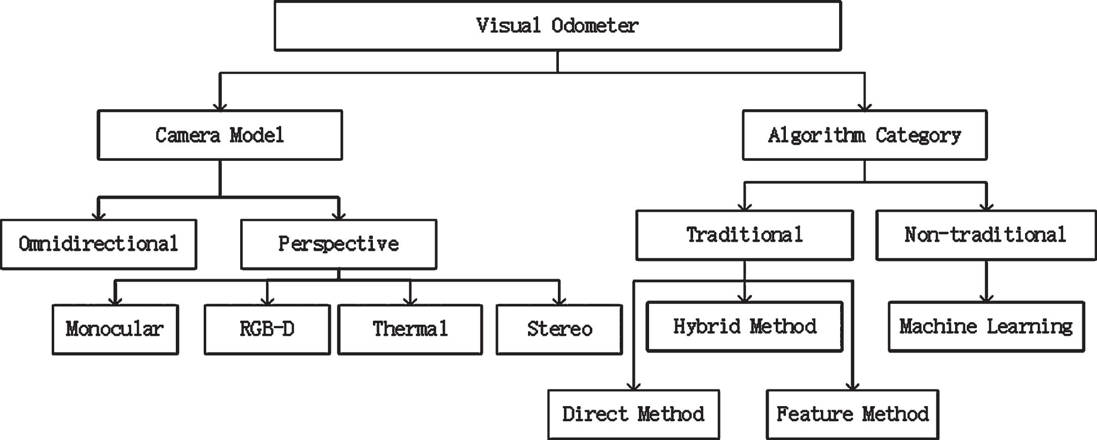
Classification and common algorithms of visual odometry.

When using machine learning methods to estimate motion parameters, most scholars directly use adjacent image sequences captured by cameras to obtain results. In the training phase, machine learning selects the required feature information to get the desired result, and then in the prediction phase, the model that has been learned is used to output the calculation result. Machine learning-based methods have also been shown to bring us many opportunities in solving geometry-based problems [7].

In summary, the existing machine learning has demonstrated its unique application advantages, at the same time, it is also faced with some difficult to solve the problem, including the efficiency or resource utilization, for the current face of some of the serious challenges, the starting point of this paper aims to solve such difficulties, which are embodied in:

Due to the difference in arithmetic power of different computers, when dealing with the problem of image sequences, processors with poorer performance often take longer time to solve the results, which also challenges our real-time performance. Therefore, we use the FLANN_PSC-RANSAC algorithm to extract feature information from image sequences, and then feed the feature pairs into machine learning to transform the image sequence problem into a text problem, which greatly improves the computational efficiency.

In addition, the direction of most scholars’ research is directed towards a specific scenario, such as a scenario with milder lighting and a cleaner site environment. However, in order to provide accurate results at all times, the case of low ambient light and messy scene environment also needs to be considered. In our system work, we have introduced the situation of darker ambient light to verify the actual effect of our framework in this working environment, to ensure that our framework can continue to work in different light environments, to achieve the effect of continuous work throughout the day.

Finally, the image sequences captured in different working environments have different characteristics, which leads to the prediction of results that do not meet our desired results, and the existing research does not further subdivide and discuss the scenes, which makes it difficult to highlight the algorithm’s generalization ability. In this paper, we validate our proposed method in different scenarios (open road, closed park, and nighttime scenarios) to demonstrate the strong generalization ability of our method.

This paper is organized as follows: Section 2 presents related work, Section 3 details the framework of our proposed system, Section 4 presents our experimental results, and finally, Section 5 presents our conclusions.

2 Related work

2.1 Visual odometry based on geometry

Geometry-based visual odometry is a process in which a camera interacts with the 3D world and provides distance information in real time, and is used in the fields of computer vision, robot navigation, and augmented vision. In the field of geometry-based visual odometry methods, feature-based methods, appearance-based methods, and hybrid methods are included. Feature-based methods involve searching for features (e.g., points, lines, corners) that are specifically and necessarily linked between sequences of consecutive images, and then solving for the position and direction of motion of the carriers through camera geometry and computer vision principles; whereas, the appearance-based approach treats all pixels of neighbouring image frames or blocks of pixels in some regions as features; moreover, the hybrid approach uses a dynamic combination of both in practical applications [8].

In the field of feature-based methods, Nister et al. first proposed a prediction system based on video input, using the matched feature pairs for calculation [2], and Nister also used the classic five-point algorithm for motion calculation [9]. To further improve the matching accuracy of feature points, Badino et al. improved the feature extraction method, incorporating previous historical data into the selection of key feature locations to improve the accuracy of calculating motion [10]. Feature-based methods are proven to be robust in the environment, and their accuracy is proportional to the number and robustness of feature pairs, and more robust feature pairs can also play a good role in feedback verification in the calculation process. Therefore, Kitt et al. combined iterative Sigma points and the RANSAC outlier rejection scheme to provide uniform and robust feature pairs [11].

In the field of direct methods, the basic principle is to use pixel intensities to perform calculations based on minimizing the luminosity difference, so its computational power is lower than that of feature-based methods [12], but it works better in low-texture environments. Vatani et al. proposed an improved appearance-based algorithm, which is selected according to the relative mask size and position changes of the vehicle, which can be pre-matched, which improves the efficiency and reliability of matching [13]. In addition, some scholars combine appearance-based methods and the visual compass to assist the work of visual odometry [14, 15].

To better combine the advantages of the two, Scaramuzza et al. proposed a hybrid algorithm, using two trackers, using the feature method to calculate the translation of the vehicle, then using the appearance method to calculate the rotation of the vehicle, and finally achieved good calculation results [16]. In addition, Feng et al. designed a parallel algorithm, which uses the threshold method to judge, and the feature number is above a certain threshold, and the feature method is used, Otherwise, the appearance method is used for calculation, which improves the generalization of the geometric method [17].

In practice, different technological approaches have different performances. The feature-based visual odometry method is more stable in practice, and it is not sensitive to the light changes in the environment, and it can still work normally when there is occlusion in part of the region, but when the physical environment features are missing or the collected image texture information is less, the number of extracted feature points is not enough to solve the required information, and when it is in a dynamic environment, if it cannot eliminate the irrelevant dynamic objects well, it may interfere with the normal extraction of feature points. In addition, the appearance-based visual odometry method is simple and intuitive to use, computationally efficient, and performs better in dynamic environments than the feature-based visual odometry method due to the absence of a tedious feature extraction process, but this method is more sensitive to light intensity and susceptible to image occlusion, which can lead to continuity interruptions. Hybrid algorithms are proposed to better exploit the advantages of both in some specific scenarios, but this also leads to an increase in the computational load of the system, which affects the real-time performance of the model. There is therefore an urgent need to develop a better fusion method that also ensures the efficiency and generalizability of the algorithm.

2.2 Visual odometry based on deep learning

The emergence of deep learning has greatly improved the reliability and generalization of the algorithms, in particular the emergence of lightweight networks that ensure high reliability while reducing the resource consumption of the algorithms, further improving their real-time performance, making machine learning methods possible for the development of visual odometry.

In 2008, Roberts et al. first proposed the use of machine learning techniques to estimate the ego-motion of mobile robots. They used independent K-Nearest-Neighbors (KNN) models to learn in blocks and then updated estimates based on the obtained scores [18]. Subsequently, Vitor et al. proposed a new framework to infer the uncertainty of the training set through a multi-output Gaussian process (GP), which in turn directly maps image features to vehicle motion [19]. With the rise and development of deep learning, in recent years, more and more scholars use deep learning to solve practical problems. Konda et al. proposed a method to build a model using a convolutional neural network CNN to estimate depth and motion information [20]. To further improve the accuracy, Grigoriev et al. proposed an integrated model of ResNet and convolutional layers under the general CNN framework to achieve end-to-end prediction results [21].

In addition, Jiao et al. used CNN and Bi-LSTM network to build the MagicVO framework to better learn the interrelationships between features [22]. Wang et al. recently proposed a new self-supervised supervised algorithm (MotionHint), trained to predict the next pose and its uncertainty [23]. Krishnan et al. proposed a feature-based deep learning method, which reads feature information through ORB and then uses the CNN-LSTM network for learning [24], however, it does not take into account the fact that the feature information is incorrectly matched in the matching process, and the stacking of neural networks greatly reduces the real-time performance of the algorithm.

Current deep learning techniques have evolved to focus on convolutional neural networks, memory neural networks, self-attention mechanism network models, and graphical neural networks, and a number of excellent improved algorithms have emerged, including ResNet (Residual Neural Network), DenseNet (Densely Connected Convolutional Networks), DenseNet (Densely Connected Convolutional Networks), and SDMT (Dependence Multi-task Transformer Network) [25 –27]. In different application scenarios, these novel networks can lead to optimal performance, but in the field of vision ranging, due to the requirement of high real-time performance, we need it to have the least time loss and the highest accuracy, so recent research still revolves around lightweight single-task neural networks that have been continuously optimized At the same time, in terms of its generalization, we also need to discuss it and propose a practical method, therefore, in this paper, we propose a method of using images collected in different environments to select feature information for training and prediction. Experiments show that our designed framework can better improve the robustness, real-time, and generalization of the VO system in practical work.

3 Methodology

This section details the approach we used and gives our thoughts. We first describe our feature information extraction method, then give the machine learning method adopted by our framework, and finally show the system framework we designed.

3.1 Feature information extraction method

In order to better verify the generalization of our proposed framework, we choose three types of scenarios for experiments, including open roads, and closed parks that are greatly affected by multipath, in addition, we also collect nighttime scenes with weak lighting environment to verify the effectiveness of our framework for such scenes. When collecting, we use the most common monocular camera for recording, which is used to record the driving images of different scenes under a certain period, and then extract the continuous image sequence that constitutes the video to ensure that the data in the input frame is a continuous and stable sequence of images.

When extracting feature point pairs, we use the FLANN_PSC-RANSAC algorithm. The reason for choosing this method is that we use the FLANN (Fast Library for Approximate Nearest Neighbors) algorithm to match and extract feature pairs in adjacent image sequences, in order to improve the accuracy, we also need to combine the PSC-RANSAC algorithm for verification to eliminate some false matches.

3.1.1 FLANN

FLANN algorithm, as a collection of nearest neighbor search algorithms for large datasets and high-dimensional features, is often used in the field of feature search. The FLANN algorithm consists of the randomized k-d tree algorithm, the priority search k-means tree algorithm and matches binary features by searching multiple hierarchical clustering trees [28].

The randomized k-d tree algorithm is an approximate nearest neighbor search algorithm. The idea of the algorithm is to construct multiple randomized k-d trees for parallel search [29]. It is worth noting that, compared with the classical k-d algorithm, its improvement lies in replacing the idea of directly dividing from the dimension with the highest variance in the classical algorithm with a random selection from the top N_D dimension with the highest variance. In addition, it sets this process up as a single priority queue, ensuring that in all tree checkpoints, once a data point has been checked by a previous tree, it will be marked for processing, avoiding double checking.

The priority search k-means tree algorithm is a kind of clustering algorithm, where k represents the number of categories, and Means represents the mean. Its algorithm idea is to divide k regions, and then recursively construct the tree after the divided regions. In the recursive process, once the data is found to be less than k, stop the recursive process and use its data node as a leaf node; then, in the search process, start the search from the root node, start to search the nearest branch, add the unexplored data nodes to the priority queue to avoid omission, and finally get the optimal clustering node.

Finally, the FLANN algorithm also introduces a cost function c (θ) for the selection of the fastest algorithm: $min_{θ \in Θ} c (θ)$ (1)

Combining the tree traversal time, build time and memory overhead, we can get the following cost function: $c (θ) = \frac{s (θ) + w_{b} b (θ)}{{min}_{θ \in Θ} (s (θ) + w_{b} b (θ))} + w_{m} m (θ)$ (2)

where s (θ), b (θ) and m (θ) represent tree traversal time, build time and memory overhead, w_b and w_m are used to denote the relative importance of build time and memory overhead in the overall cost. The memory overhead m (θ) is calculated from the memory used by the tree and the memory used by the data: $m (θ) = \frac{m_{t} (θ)}{m_{d}}$ (3)

3.1.2 PSC-RANSAC

When using the FLANN algorithm to extract feature information, we found that there are inevitably some false matches. To maintain the robustness of our algorithm, we introduced the PSC-RANSAC algorithm. The PSC-RANSAC algorithm, proposed by Ma et al., aims to use the Density Peak Clustering (DPC) algorithm to more robustly eliminate false matches in the matching results, and its results have also been shown to be more effective than the standard RANSAC algorithm [30].

The Random sample consensus (RANSAC) algorithm refers to a method of estimating a mathematical model through an iterative method of randomly extracting data from a set of observational data containing errors and then eliminating erroneous data. The basic idea of the PSC-RANSAC algorithm is to judge the effect after the RANSAC matching result is obtained. If there are wrong matches in RANSAC matching results and cannot be filtered out, DPC is used for secondary matching.

In the working process of the camera, the combination of translation and rotation is generally included, so the PSC-RANSAC method splits this process into rotation first and then translation. The PSC-RANSAC algorithm believes that during the rotation process, the offset of the feature points is only determined by the rotation radius, so the feature points of the same cluster should have the same pixel offset, to toe the mismatched points in the same cluster. Similarly, the author found that in the process of translation, the pixel offset has a negative correlation with the depth, so the feature points in the same cluster should also have similar offsets. Based on this logic, PSC-RANSAC can more accurately divide and process the data initially screened by RANSAC to eliminate mismatched feature pairs. The cluster center is considered to be surrounded by a number of low-density points, namely: $\begin{matrix} point i = \\ {\begin{matrix} a cluster center & ρ_{i} > ρ_{c} & δ_{i} > δ_{c} \\ a isolate cluster center & ρ_{i} < ρ_{ic} & δ_{i} > δ_{ic} \end{matrix} \end{matrix}$ (4) where ρ_i is the local density of the cluster center, ρ_c, ρ_ic represent the density threshold of the cluster center and the density threshold of the isolated center. δ_i is the distance from the point to the cluster center, δ_c, δ_ic represent the distance threshold of the cluster center and the distance threshold of the isolated center. ρ_i is calculated as follows: $ρ_{i} = \sum_{{i} / - j \in l_{s}} e^{- {(\frac{d_{ij}}{d_{c}})}^{2}}$ (5)

Where d_ij is the distance between two points and d_c is the cut-off distance.

Thus, cluster centers include points with high ρ_i and high δ_i, isolated centers include points with low ρ_i and high δ_i.

3.1.3 FLANN_PSC-RANSAC

Although the FLANN algorithm has a very powerful feature matching function, it is not able to effectively reject the incorrect feature pair information it matches, which greatly affects the recovery effect of the subsequent trajectory. Therefore, after the matching and extraction of feature information by FLANN, the PSC-RANSAC algorithm is used for verification, which on the one hand can eliminate some feature pairs of information with lower reliability, and on the other hand can reduce the algorithm’s dependence on computing power, reduce the algorithm’s power consumption, and ensure that the algorithm’s real-time performance is guaranteed.

As shown in Fig. 2, we compared the feature pair extraction effect using the FLANN algorithm and the FLANN_PSC-RANSAC algorithm. To better reflect our advantages, we deliberately select moving objects whose speed is not much different from ours, although our displacement changes in adjacent image sequences are not obvious, due to the difference in our speed, our relative position has been changing. If we also incorporate the feature pair information of the moving object into our framework, it will inevitably affect our accuracy. From Fig. 2, we can see that our feature extraction method can find this situation well, and discard the wrong feature information in time to avoid the impact of wrong matching on us. Algorithm 1 shows the detailed pseudo-code of the algorithm.

Fig. 2

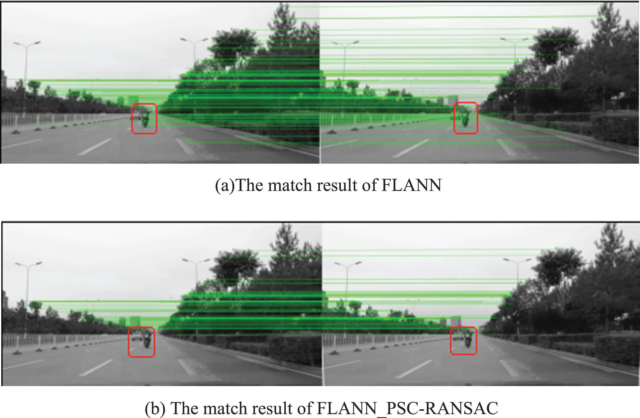
Comparison of extraction effect between FLANN algorithm and FLANN_PSC-RANSAC feature.

Algorithm 1: FLANN_PSC-RANSAC.
Input: Continuous image sequence data.
FLANN feature search:
1. Calculate m (θ) by (3).
2. Calculates (θ), b (θ) and m (θ).
3. Calculate c (θ) by (2) for selection algorithm.
4. If c_k-d (θ) ⩽ c_k-mens (θ)
Selection of the randomized k-d tree.
Else selection of the priority search k-means tree algorithm.
5. Extract feature information.
PSC-RANSAC feature detection:
1. RANSAC rejects false matches.
2. Calculate ρ_i by (5) and δ_i.
3. If ρ_i > ρ_c
δ_i > δ_c
As the cluster center
Else if ρ_i < ρ_c
δ_i > δ_ic
As the isolate cluster center.
4. Secondary rejection of false matches.
Output: Reliable feature pair information.

We combine the two and use the FLANN_PSC-RANSAC algorithm to ensure that the feature pairs we match have good accuracy, and at the same time to ensure the real-time performance of our algorithm, making our subsequent processing data more reliable.

3.2 LSTM

In our framework, we employ a long short-term memory artificial neural network for algorithm learning and outcome prediction. This section describes the structure and working of LSTMs.

The LSTM network structure was proposed by Sepp Hochreiter et al. and has been used until now [31]. It appeared to solve the problem of a long-term dependence on RNNs. Its success is due to its introduction of a gate mechanism, which enables it to better learn previous features, thereby avoiding the feature forgetting problem caused by forwarding propagation. As shown in Fig. 3, we show the detailed structure of LSTM.

Fig. 3

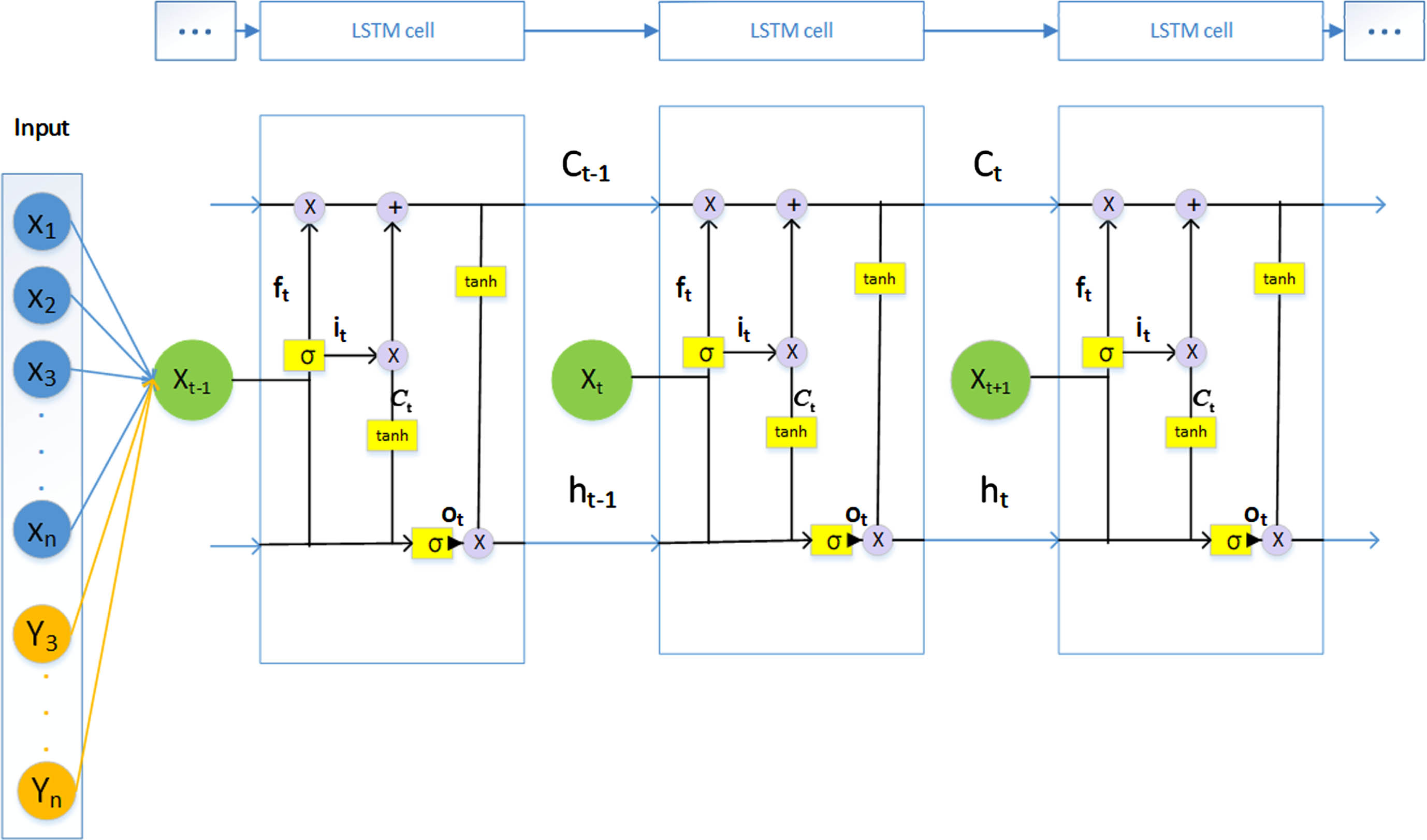
LSTM network structure.

In general, there is a linear or nonlinear relationship between the output of LSTM and the input: $C_{t} = f_{t} \times C_{t - 1} + i_{t} \times {\tilde{C}}_{t}$ (6) where f_t is the most important mechanism forgetting gate in LSTM, which controls the result between [0, 1] through the σ activation function: $σ (x) = \frac{1}{1 + e^{- x}}$ (7) $f_{t} = σ (W_{f} \cdot [h_{t - 1}, x_{t}] + b_{f})$ (8)

In addition, the input gate in LSTM is represented by i_t, and its function is to decide which features in ${\tilde{C}}_{t}$ are used to update C_t, which is calculated by x_t and h_t-1 through the activation function σ: $i_{t} = σ (W_{i} \cdot [h_{t - 1}, x_{t}] + b_{i})$ (9)

We call ${\tilde{C}}_{t}$ the cell state update value, which is calculated by x_t and h_t-1 through the activation function tanh: ${\tilde{C}}_{t} = tanh (W_{c} \cdot [h_{t - 1,} x_{t}] + b_{c})$ (10)

The output gate in LSTM is represented by o_t, and the calculation method of o_t is the same as the forgetting gate and the input gate: $o_{t} = σ (W_{o} \cdot [h_{t - 1}, x_{t}] + b_{o})$ (11)

The final output result h_t is represented by the output gate o_t and the cell state C_t:

$h_{t} = o_{t} \times tanh (C_{t})$ (12)

In the process of input, we input our feature pair data and the six-degree-of-freedom attitude matrix simultaneously in the order of time series, and let the LSTM network learn the nonlinear relationship between them, the important thing is to use the advantages of LSTM to process time series, and finally achieve the effect of high-precision prediction through the training of a large amount of data. Figure 4 is the flow of our data processing with LSTM.

Fig. 4

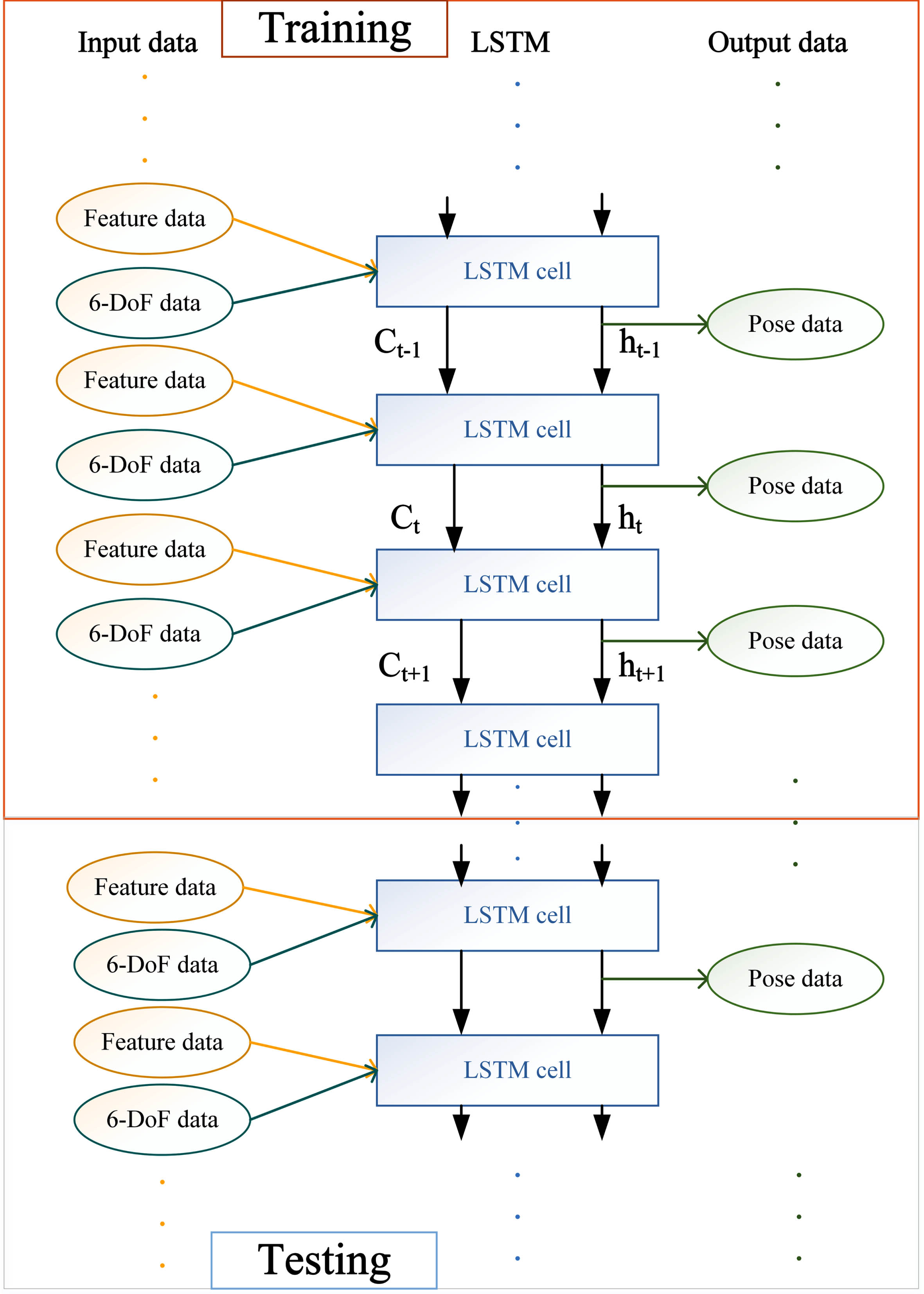
LSTM processing data flow.

3.3 System framework

Our system includes a feature extraction subsystem and an LSTM network prediction subsystem. In the feature extraction subsystem, we perform a pre-processing operation on the video information captured by the device to convert it into a continuous sequence of images. First, the image sequence is screened to remove some distortions and blurred images, which are fed into the feature extraction subsystem, specifically including the matching and extraction of feature information by FLANN, and then the extracted feature information is rejected by using the PSC-RANSAC algorithm, which includes the classification of clustering centers and the elimination of outliers, and finally the obtained feature pairs of information are fed into the LSTM network prediction subsystem to perform the next operation.

As shown in Fig. 5, when processing, we can find that there are obvious differences in the number of feature pairs in different scenarios, that is, the closed park has more identifiable feature points, so the matched feature pairs are the most; on open roads, street sign trees are the main ones, followed by the number. Finally, we found that the number of feature pairs in the collected nighttime images is relatively small compared with the first two, but due to our troubleshooting algorithm, the accuracy of feature pair matching can still be guaranteed even in the case of strong exposure or no illumination of street lights.

Fig. 5

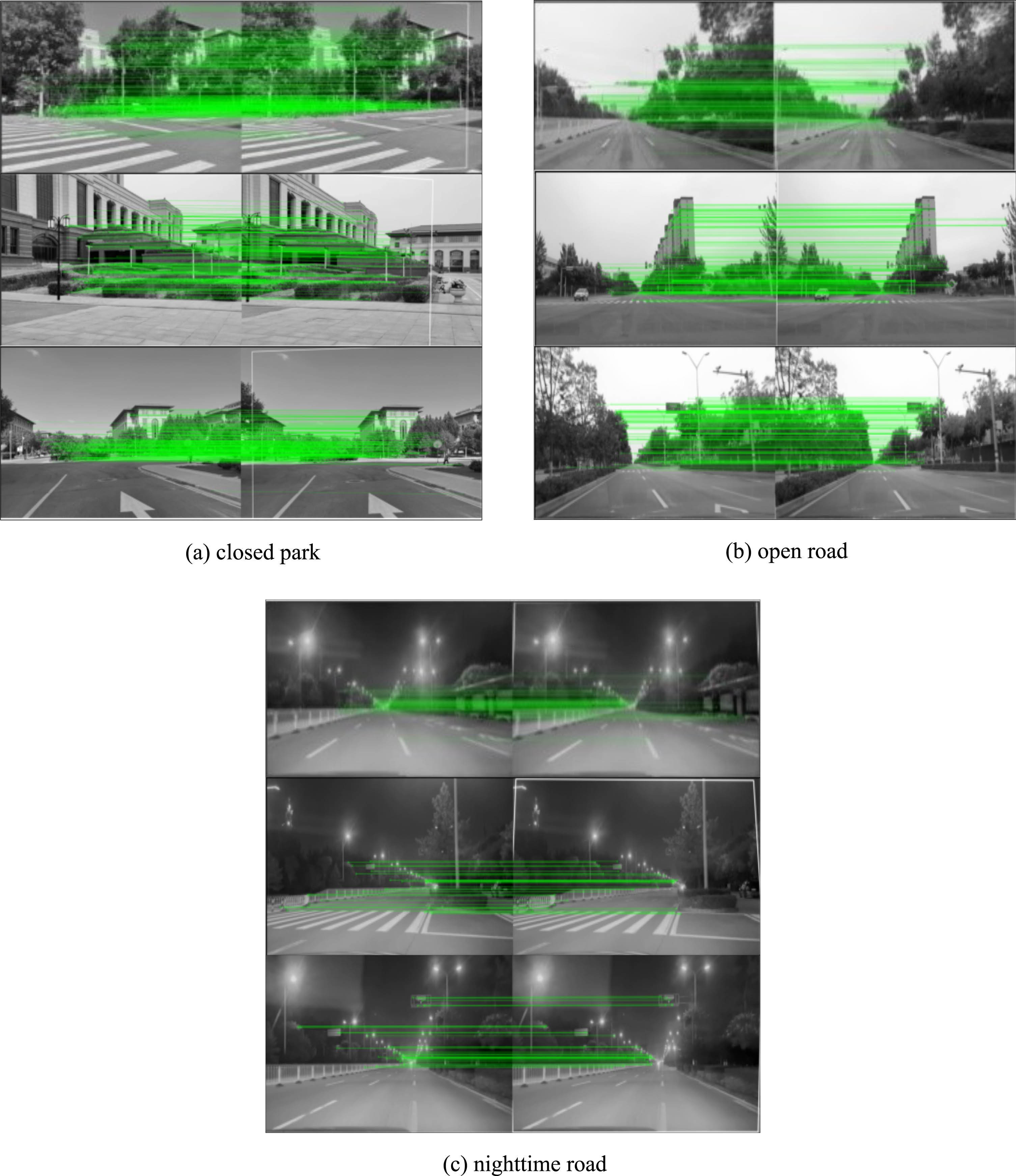
Feature pair matching effect in different scenarios.

In the LSTM network prediction subsystem, we further divide it into a training module and a testing module. In the training module, we match the six-degree-of-freedom information collected in advance with the image frame data, which is handed over to the LSTM network for pre-learning, and after a large number of training processes, we test it with the generated model, which ensures that the algorithm can work with the offline model at any time, reduces the algorithm’s dependence on the platform, and is capable of independently and accurately outputting the vehicle’s moving attitude information. The overall system framework design is shown in Fig. 6.

Fig. 6

System framework.

4 Experimental results

In this section, we introduce our training and testing, comparing the performance of the proposed algorithm with other algorithms in terms of accuracy.

To better verify our proposed algorithm, we divided the dataset into three types, namely open roads, closed parks, and night scenes with weak lighting environments, to prove whether our algorithm has strong generalization and robustness. Since our goal is to enable the visual odometry to operate stably in all-weather scenarios, introducing these three scenarios can also observe whether they can be flexibly converted in different environments, while ensuring the accuracy of the model.

4.1 Training

The accuracy of the data during training will directly affect the robustness of the future model. To learn more data from different scenarios during training, we introduce data from multiple scenarios for the model to learn. The learning rate is one of the most important hyperparameters in deep learning. We choose an initial learning rate of 0.003 for learning. Then, we choose the Adam optimizer for optimization, Adam optimizer absorbs the advantages of Adaptive Learning Rate and Gradient Algorithm (Adagrad) and momentum gradient descent algorithm, therefore, it has both the advantages of the former to adapt to sparse gradients and the latter’s advantages of mitigating gradient oscillations.

In the training process, we will match the matched feature information with the pose data, and then the model will learn and calculate the predicted results and the results we input to obtain our loss function. To avoid the impact of overfitting, we also set a threshold, when the loss function is lower than the specified threshold, it will stop in advance, which better guarantees the effect of future prediction.

4.2 Testing

After training the model, in Fig. 7 we first select our most common travel directions as tests, namely straight and turn, to see how our framework performs when dealing with the two situations. From Fig. 7, we can see that our results are not only biased towards the true trajectory but also its divergence is not obvious.

Fig. 7

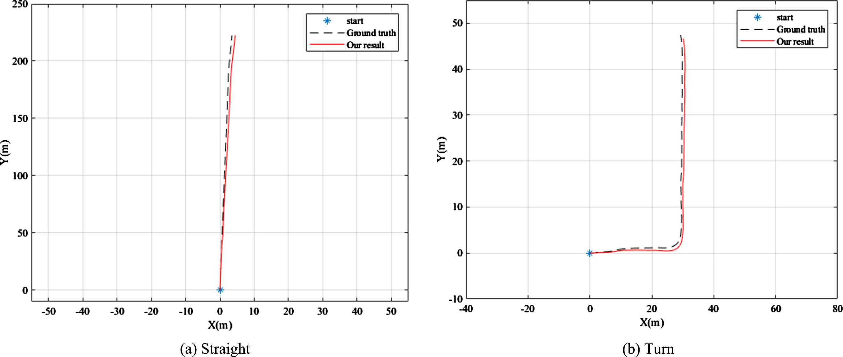
Common travel direction test results.

Then, to better compare the effects of our long-term work, we introduce several other neural network-based end-to-end monocular visual odometry for comparison, and we still choose datasets of different scenes as validation sets. Figure 8 and Table 1 show the performance of our model under different open roads, Table 1 derived from quantitative experiments, analyzes our translation and rotation performance using mean root mean square error (RMSE), then relies on our results to recover the action trajectory and show it in Fig. 8. We can see that our framework demonstrates its strengths in all of the open roads, providing more robust results relative to CNN-LSTM-VO, CNN-VO and CNN-BiLSTM-VO.

Fig. 8

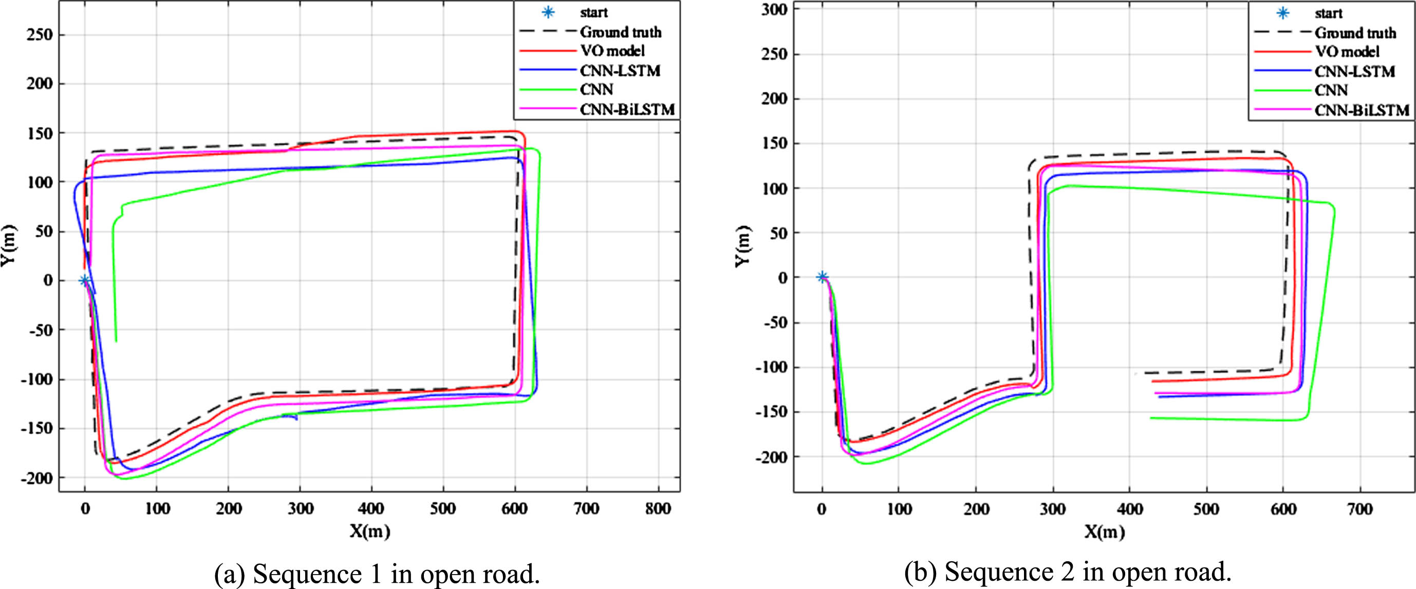
Trajectory recovery performance under different open roads.

Table 1

Performance under different open roads

Seq.	01		02
	t (%)	r (°)	t (%)	r (°)
VO model	4.13	1.60	4.57	1.81
CNN-LSTM-VO	14.62	2.75	12.46	2.11
CNN-VO	16.18	2.25	18.05	3.42
CNN-BiLSTM-VO	5.06	1.94	8.64	2.07

t (%): The RMSE of translation. r (°): The RMSE of rotation.

Subsequently, in Fig. 9 and Table 2, we show the performance of our framework on closed campuses, Since the scene characteristics of the closed park are different from those of the open road, to be able to observe our effects more realistically, the trajectory of the closed park is also longer and more complicated. In the recovered trajectory, it can be seen that the other three methods do not differ too much in their actual results, since they are all based on the feature information extracted from the CNNs for the prediction, and we also note that due to the stacking of the neural networks, it is not a small challenge for the power consumption of our platform.

Fig. 9

Trajectory recovery performance under different roads in closed parks.

Table 2

Performance under different roads in the closed park

Seq.	03		04
	t (%)	r (°)	t (%)	r (°)
VO model	3.06	1.65	2.62	1.94
CNN-LSTM-VO	5.71	2.16	10.22	2.95
CNN-VO	8.30	1.58	19.62	2.66
CNN-BiLSTM-VO	6.13	2.09	11.51	2.57

t (%): The RMSE of translation. r (°): The RMSE of rotation.

In Fig. 10 and Table 3, we show the effect of the night scene where, to better demonstrate the effect, we have Sequence 5 on the same route as Sequence 1. From this, we can clearly see that other networks are not as good as well-lit scenes when dealing with night scenes, but our framework gives satisfactory results, this is because our preprocessing process eliminates the influence of illumination on the data, so that the framework does not need to learn the characteristics of night scenes during the training process, and it also ensures the robustness of our framework in night scenes. In addition, to verify the generalizability claimed in this paper, we introduced more complex nighttime scenarios (Sequence 6 & Sequence 7), which were not only tested on the basis of nighttime scenarios, but also the trajectories of the sports cars were more variable. Similarly, after our rigorous pre-processing, our model still stabilizes the accuracy within an acceptable range, whereas the other methods are less effective and their accuracy continues to degrade over time.

Fig. 10

Trajectory recovery performance in the nighttime environment.

Table 3

Performance in a nighttime environment

Seq.	05	06	07
	t (%)	r (°)	t (%)	r (°)	t (%)	r (°)
VO model	5.12	2.04	3.16	1.49	2.57	1.18
CNN-LSTM-VO	16.23	2.33	19.41	1.95	13.25	2.74
CNN-VO	36.18	3.05	15.85	2.06	19.50	2.94
CNN-BiLSTM-VO	10.27	2.29	28.43	2.59	4.10	1.97

t (%): The RMSE of translation. r (°): The RMSE of rotation.

5 Conclusion

This paper proposes a continuous and generalized monocular visual odometry method based on features and neural networks. The FLANN_PSC-RANSAC algorithm is used to extract the feature pairs of adjacent image sequences, and the error matching algorithm is used to remove the error matching, which ensures the reliability of the neural network model, compared with other monocular visual odometry methods, the accuracy of the algorithm is further improved, and good results are also achieved in the trajectory recovery stage.

In addition, through comparative experiments in different environments (open roads, closed parks), it is found that our algorithm has strong generalization, and it still maintains its algorithm accuracy for different scenarios. Finally, we introduce the case of the poor lighting environment, and it is found that due to our advanced preprocessing process, the robustness of the algorithm under different lighting conditions is guaranteed.

It is worth noting that visual odometers require high processing efficiency to ensure the provision of continuous and reliable operating parameters for the vehicle in motion, which is one of the important implications of the research in this paper. In the overall design of our algorithm, the real-time performance of the algorithm is well ensured due to the low resources required in the prediction phase, and in our future work we will focus on exploring the impact of other external information on the prediction results to further improve the accuracy of our algorithm.

References

Moravec

H.P.

, Obstacle Avoidance and Navigation in the Real World by a Seeing Robot Rover, Stanford University 1980.

Nister

, Naroditsky

, Bergen

, Visual odometry, Proceedings of the 2004 IEEE Computer Society Conference on Computer Vision and Pattern Recognition. CVPR 2004., (2004), pp. I–I.

Smith

, Self

, Cheeseman

, Estimating Uncertain Spatial Relationships in Robotics. In: Cox, I.J., Wilfong, G.T. (eds) Autonomous Robot Vehicles. Springer, New York, NY, (1990), pp. 167–193.

Poddar

, Kottath

, Karar

, Motion Estimation Made Easy: Evolution and Trends in Visual Odometry. In: Hassaballah, M., Hosny, K. (eds) Recent Advances in Computer Vision. Studies in Computational Intelligence, (2019), pp. 305–331.

Wang

, Ma

, Chen

, Ren

and Lu

, Approaches, Challenges, and Applications for Deep Visual Odometry: Toward Complicated and Emerging Areas, IEEE Transactions on Cognitive and Developmental Systems 14 (2020), 35–49.

Alkendi

, Seneviratne

and Zweiri

, State of the Art in Vision-Based Localization Techniques for Autonomous Navigation Systems, IEEE Access 9 (2021), 76847–76874.

Wang

, Clark

, Wen

and Trigoni

, End-to-end, sequence-to-sequence probabilistic visual odometry through deep neural networks, The International Journal of Robotics Research 37 (2018), 513–542.

Scaramuzza

and Fraundorfer

, Visual Odometry [Tutorial], IEEE Robotics & Automation Magazine 4(18) (2011), 80–92.

Nister

, An efficient solution to the five-point relative pose problem, IEEE Transactions on Pattern Analysis and Machine Intelligence 6(26) (2004), 756–770.

10.

Badino

, Yamamoto

, Kanade

, Visual Odometry by Multi-frame Feature Integration, in: 2013 IEEE International Conference on Computer Vision Workshops (2013), pp. 222–229.

11.

Kitt

, Moosmann

, Stiller

, Moving on to dynamic environments: Visual odometry using feature classification, in 2010 IEEE/RSJ International Conference on Intelligent Robots and Systems (2010), pp. 5551–5556.

12.

Engel

, Koltun

and Cremers

, Direct Sparse Odometry, IEEE Transactions on Pattern Analysis and Machine Intelligence 3(40) (2018), 611–625.

13.

Nourani-Vatani

, Roberts

, Srinivasan

M.V.

, Practical visual odometry for car-like vehicles, in 2009 IEEE International Conference on Robotics and Automation (2009), pp. 3551–3557.

14.

Labrosse

, The visual compass: Performance and limitations of an appearance-based method, Journal of Field Robotics 23(10) (2006), 913–941.

15.

Gonzalez

, Rodriguez

, Guzman

, Pradalier

and Siegwart

, Combined visual odometry and visual compass for off-road mobile robots localization, Robotica 30(6) (2012), 865–878.

16.

Scaramuzza

and Siegwart

, Appearance-Guided Monocular Omnidirectional Visual Odometry for Outdoor Ground Vehicles, IEEE Transactions on Robotics 5(24) (2008), 1015–1026.

17.

Feng

, Zhang

, Sun

, Song

, A fusion algorithm of visual odometry based on feature-based method and direct method, in 2017 Chinese Automation Congress (CAC) (2017), pp. 1854–1859.

18.

Roberts

, Nguyen

, Krishnamurthi

, Balch

, Memory-based learning for visual odometry, in 2008 IEEE International Conference on Robotics and Automation, (2008), pp. 47–52.

19.

Guizilini

, Ramos

, Semi-parametric models for visual odometry, in 2012 IEEE International Conference on Robotics and Automation, (2012), pp. 3482–3489.

20.

Konda

, Memisevic

, Unsupervised learning of depth and motion. arXiv preprint arXiv:1312.3429 (2013).

21.

Grigorev

, Jiang

, Rho

, et al., Depth estimation from single monocular images using deep hybrid network, 76 (2017), 18585–18604.

22.

Jiao

, Jiao

, Mo

, Liu

and Deng

, MagicVO: An End-to-End Hybrid CNN and Bi-LSTM Method for Monocular Visual Odometry, IEEE Access 7 (2019), 94118–94127.

23.

Wang

, Wang

Y.-P.

, Manocha

, MotionHint: Self-Supervised Monocular Visual Odometry with Motion Constraints, in 2022 International Conference on Robotics and Automation (ICRA), (2022), pp. 1265–1272.

24.

Krishnan

K.S.

, Sahin

, ORBDeepOdometry - A Feature-Based Deep Learning Approach to Monocular Visual Odometry, in 2019 14th Annual Conference System of Systems Engineering (SoSE), (2019), pp. 296–301.

25.

He , Kaiming ,et al., Deep residual learning for image recognition, in Proceedings of the IEEE Conference on Computer Vision and Pattern Recognition (2016), pp. 770–778.

26.

Huang

, Liu

, Van Der Maaten

,et al., Densely connected convolutional networks, in Proceedings of the IEEE Conference on Computer Vision and Pattern Recognition (2017), pp. 4700–4708.

27.

, Lv

, Li

,et al., SDMT: Spatial Dependence Multi- Task Transformer Network for 3D Knee MRI Segmentationand Landmark Localization. In IEEE Transactions on Medical Imaging (2023), pp. 2274–2285.

28.

Muja

and Lowe

D.G.

, Scalable Nearest Neighbor Algorithms for High Dimensional Data, IEEE Transactions on Pattern Analysis and Machine Intelligence 11(36) (2014), 2227–2240.

29.

Silpa-Anan

, Hartley

, Optimised KD-trees for fast image descriptor matching, in 2008 IEEE Conference on Computer Vision and Pattern Recognition (2008), pp. 1–8.

30.

, et al., An image matching optimization algorithm based on pixel shift clustering RANSAC, Information Sciences 562 (2021), 452–474.

31.

Hochreiter

and Schmidhuber

, Long Short-Term Memory, Neural Computation 8(9) (1997), 1735–1780.

Continuous and generalized visual odometry based on FLANN_PSC-RANSAC_LSTM

Abstract

Keywords

1 Introduction

2.1 Visual odometry based on geometry

2.2 Visual odometry based on deep learning

3 Methodology

3.1 Feature information extraction method

3.1.1 FLANN

4.1 Training

4.2 Testing

References