SGCRNN: A ChebNet-GRU fusion model for eeg emotion recognition

Abstract

The paper proposes a deep learning model based on Chebyshev Network Gated Recurrent Units, which is called Spectral Graph Convolution Recurrent Neural Network, for multichannel electroencephalogram emotion recognition. First, in this paper, an adjacency matrix capturing the local relationships among electroencephalogram channels is established based on the cosine similarity of the spatial locations of electroencephalogram electrodes. The training efficiency is improved by utilizing the computational speed of the cosine distance. This advantage enables our method to have the potential for real-time emotion recognition, allowing for fast and accurate emotion classification in real-time application scenarios. Secondly, the spatial and temporal dependence of the Spectral Graph Convolution Recurrent Neural Network for capturing electroencephalogram sequences is established based on the characteristics of the Chebyshev network and Gated Recurrent Units to extract the spatial and temporal features of electroencephalogram sequences. The proposed model was tested on the publicly accessible dataset DEAP. Its average recognition accuracy is 88%, 89.5%, and 89.7% for valence, arousal, and dominance, respectively. The experiment results demonstrated that the Spectral Graph Convolution Recurrent Neural Network method performed better than current models for electroencephalogram emotion identification. This model has broad applicability and holds potential for use in real-time emotion recognition scenarios.

Keywords

Electroencephalogram emotion recognition chebyshev network gated recurrent units spectral graph convolution recurrent neural network adjacency matrix

1 Introduction

Emotion recognition has become a research focus in the fields of psychology, neuroscience, and medicine [1]. In order to accurately capture and interpret human emotions, researchers have adopted various measurement methods, primarily including audiovisual techniques and physiological techniques [2]. Audiovisual techniques rely on external expressions such as facial expressions, language, and gestures, which are prone to overlooking subtle emotions and are influenced by human control and deception. In contrast, physiological techniques based on electroencephalography (EEG) provide a more reliable and objective approach to emotion recognition [3]. As a result, there has been increasing attention to emotion recognition based on EEG signals.

Mehrabian expanded the emotion model from two-dimensional to three-dimensional [4]. The three-dimensional emotion model includes the addition of dominance to the V-A model initially proposed by Russel [5]. It involves describing the emotional state of individuals based on three dimensions: valence (i.e., calm/excited), arousal (i.e., unpleasant/pleasant), and dominance (i.e., uncontrollable/controllable). This study employs a three-dimensional emotion model to evaluate the classification performance of the system. This model provides a more comprehensive representation of emotions and possesses enhanced capabilities for emotion analysis.

Deep learning methods have been widely applied in emotion recognition research based on EEG. Due to the temporal characteristics of EEG signals, some researchers utilize recurrent convolutional networks to capture the temporal dependencies of EEG signals and better explore the temporal correlations within the signals. Chowdary, MK et al. used three architectures, Recurrent Neural Network (RNN), Long Short Term Memory (LSTM), and Gated Recurrent Unit (GRU), to identify emotions with EEG signals. It was finally concluded that RNN improved the recognition results compared with traditional classification methods [6].

However, these methods focus solely on temporal features while neglecting the spatial dimension. Xu, GX et al. introduced a hybrid GRU and CNN deep learning framework called GRU-Conv to extract critical spatial and temporal features from EEG data, with an average accuracy of 70.07% on the DEAP dataset Valence [7]. In reality, the distribution of EEG channels is not grid-like but rather exhibits irregular connections. This poses limitations for CNN in capturing structural information from the electrodes.

To overcome this issue, researchers have proposed methods to construct complex brain networks, where electrodes are abstracted as nodes and their connections are abstracted as edges. Graph Neural Network (GNN) can be utilized to learn from this type of graph-structured data. Zhu et al. [8] and Yin et al. [9] employed distance-based approaches using GCN to explore the relationships among EEG channels. However, compared to computationally intensive Euclidean distance, cosine similarity is more suitable for describing the directionality and correlation between channels. Demir et al. [10] proposed the EEG-GNN algorithm, which utilizes one-dimensional convolution in the temporal dimension to calculate Pearson correlation coefficients and employs them as functional connection weights, achieving superior classification performance compared to CNN architectures. However, the Pearson correlation coefficient is primarily suitable for measuring linear correlations and may not accurately capture the similarity of signals with non-linear relationships. To overcome this issue, this study employs cosine similarity to construct the adjacency matrix of EEG signals. Cosine similarity does not rely on the assumption of linear correlation in signals, resulting in higher computational efficiency as it only involves inner product operations between vectors. This approach is applicable to real-time systems and enables better capture of the similarity between signals.

To overcome the limitations of existing techniques, this paper proposes a deep learning model called Spectral Graph Convolutional Recurrent Neural Network (SGCRNN) based on ChebNet and GRU, specifically designed for emotion recognition from multi-channel EEG data. The SGCRNN model effectively extracts the spatiotemporal features of EEG signals and captures the local relationships between channels. In this study, ChebNet approximates graph convolutional operations using Chebyshev polynomials, enabling the effective capture of local relationships among nodes in the graph data. Modeling these local relationships is crucial for capturing channel-to-channel correlations in EEG signals and facilitates the extraction of more accurate feature representations. The main contributions of this paper are as follows:

By utilizing the cosine similarity of the spatial positions of the EEG electrodes, it is possible to capture the local relationships between EEG channels more accurately. This method takes advantage of the computational efficiency of cosine distance, effectively reducing training time, and enhancing its practicality and value in real-time monitoring applications.

The use of ChebNet as a replacement for matrix multiplication in the GRU network, along with the utilization of Chebyshev polynomials for local approximation, avoids explicit matrix multiplication operations. This approach benefits the model’s complexity and computational efficiency. This method contains the advantages of the Chebyshev network for extracting spatial features of EEG sequences and also utilizes the features of GRU for extracting EEG sequences. SGCRNN solves the problem of the weak spatial feature extraction ability of RNN, achieving full capture of the spatial and temporal dependence of EEG sequences.

This study proposes preprocessing methods such as time slicing and data augmentation and demonstrates their effectiveness through ablation experiments. By comparing with other models, the results show that the SGCRNN method achieves superior emotion recognition performance in the three-dimensional emotion model. These experiments validate the effectiveness and superiority of the novel method proposed in this paper.

2 Related work

2.1 Feature extraction

In emotion recognition research, commonly used representative EEG features are shown in Table 1. Despite the existence of various manually extractable EEG features, these traditional handcrafted features are based on a significant accumulation of domain knowledge, thus increasing the learning cost for researchers. Furthermore, most of the current neural signal features are still based on traditional time-series signal analysis theories and methods. However, the correlation between these signal features and emotional states remains unclear and requires further exploration, with certain limitations in their effectiveness.

Table 1
Common methods for EEG feature extraction

Feature type Extracted features

Time+Frequency Domain Features 1. Peak-to-Peak Interval. 2. Mean Square Value. 3. Variance. 4. Mean Value. 5. Skewness. 6. Kurtosis. 7. 1st/2nd Difference. 8. Hjorth Parameter: Mobility, Complexity, Activity. 9. Higher-order Crossing. 10. Maximum Power Spectral Frequency. 11. Power Sum. 12. Maximum Power Spectral Density. 13. Wavelet Energy. 14. Wavelet Entropy. 15. Amplitude and latency of ERPs. 16. Shannon Entropy.

Nonlinear dynamical system features 1. Approximate Entropy. 2. C0 Complexity. 3. Correlation Dimension. 4. Kolmogorov Entropy. 5. Lyapunov Exponent. 6. Permutation Entropy. 7. Singular Entropy. 8. Spectral Entropy. 9. Sample Entropy. 10. Differential Entropy. 11. Fractal Dimension. 12. Hurst Exponent. 13. Lyapunov Complexity. 14. Recurrence Plot: recurrence rate, determinism, entropy, averaged diagonal length, length of the longest diagonal line, laminarity, trapping time, length of the longest vertical line, recurrence time of 1st type, recurrence time of 2nd type.

Brain asymmetry features 1. Difference Between Channels. 2. Ratio Between Channels. 3. Asymmetry Index (AsI).

Feature type	Extracted features
Time+Frequency Domain Features	1. Peak-to-Peak Interval. 2. Mean Square Value. 3. Variance. 4. Mean Value. 5. Skewness. 6. Kurtosis. 7. 1st/2nd Difference. 8. Hjorth Parameter: Mobility, Complexity, Activity. 9. Higher-order Crossing. 10. Maximum Power Spectral Frequency. 11. Power Sum. 12. Maximum Power Spectral Density. 13. Wavelet Energy. 14. Wavelet Entropy. 15. Amplitude and latency of ERPs. 16. Shannon Entropy.
Nonlinear dynamical system features	1. Approximate Entropy. 2. C0 Complexity. 3. Correlation Dimension. 4. Kolmogorov Entropy. 5. Lyapunov Exponent. 6. Permutation Entropy. 7. Singular Entropy. 8. Spectral Entropy. 9. Sample Entropy. 10. Differential Entropy. 11. Fractal Dimension. 12. Hurst Exponent. 13. Lyapunov Complexity. 14. Recurrence Plot: recurrence rate, determinism, entropy, averaged diagonal length, length of the longest diagonal line, laminarity, trapping time, length of the longest vertical line, recurrence time of 1st type, recurrence time of 2nd type.
Brain asymmetry features	1. Difference Between Channels. 2. Ratio Between Channels. 3. Asymmetry Index (AsI).

High-level cognitive functions rely on subtle coordination between local and global brain activities, which are closely related to the network of neurons and brain regions [11]. There is inherent correlation in the brain electrical signals originating from different brain regions, making the study of brain networks a topic of extensive interest [12]. J. Jia et al. proposed a method that combines the distance and functional connectivity between EEG channels to construct a graph network for emotion classification in a two-dimensional emotion model [13]. However, calculating Pearson correlation coefficients and Euclidean distances is relatively complex, requiring consideration of multiple factors such as means and standard deviations. In contrast, cosine similarity calculations are relatively simple and efficient, involving only inner products between vectors. This makes cosine similarity advantageous for processing large-scale data and real-time systems.

The brain network constructed using cosine similarity reflects the coupling correlation between two EEG channels, making it insensitive to amplitude changes. This characteristic reduces the impact of inter-individual differences and helps establish robust and accurate EEG-based recognition models. Considering these factors, this study chooses the method of constructing brain networks using cosine similarity for extracting emotional features from EEG signals.

2.2 Latest research method

Hand-engineered approaches have certain limitations in the analysis of EEG signals for emotion recognition. Firstly, they rely on domain knowledge, which restricts their generalizability and applicability. Secondly, these methods often focus only on local feature extraction and fail to capture the global dynamics and spatiotemporal relationships of EEG signals comprehensively. Moreover, handcrafted methods have limited expressive power, which may result in the loss of important information and affect the accuracy of emotion classification. They are also highly dependent on specific tasks and datasets, making them less applicable to new tasks and datasets. Lastly, manual operations and subjectivity can lead to uncertainties and irreproducibility. To overcome these limitations, exploring methods based on machine learning and deep learning can automatically learn relevant features and patterns in EEG signals, thereby improving the accuracy and generalization capability of emotion analysis.

EEG signals are a type of sequential data, and the memory units and temporal feedback connections in RNN enable it to effectively handle the temporal characteristics of the signals. Moreover, the emotional information in EEG signals may be influenced by long-term dependencies, and RNN can capture such dependencies and model the emotional features more effectively. Therefore, many researchers choose to apply RNN in the study of EEG-based emotion recognition. J. X. CHEN et al. proposed a hierarchical bidirectional recurrent unit with an attention GRU network for human emotion classification from continuous EEG signals. The model showed a more robust classification performance than the baseline LSTM model [14]. However, in EEG signals, the arrangement of electrodes forms spatial relationships, which would be overlooked if only RNN is used for analysis. To fully leverage the spatial information in EEG signals, we can introduce CNN, which can effectively capture the local spatial features in EEG signals.

Through CNN, we can extract local spatial features from EEG signals, such as the correlation between electrodes and the topological structure. This helps to analyze the emotional content of EEG signals more accurately. S Tripathi et al. investigated two neural network models, a simple Deep Neural Network (DNN) and a CNN, to categorize user emotions by EEG signals. It showed that neural networks could effectively classify brain signals that outperform traditional methods [15]. Yang et al. proposed a method based on a multicolumn CNN algorithm that can classify emotions based on EEG signals obtained from a DEAP database [16]. Liao et al. extracted statistical features of EEG and sent them to CNN, and the accuracy of Valence in binary classification reached 81.4% [17]. Salama et al. used a 3D-CNN deep learning architecture to extract spatiotemporal features from EEG signals and proposed a combination of data augmentation and integrated learning techniques to obtain the final fusion prediction [18]. Cui et al. proposed a emotion recognition method based on two-dimensional convolution neural networks and three-dimensional convolution neural networks, called ResNeXt Attention 2D-3D Convolutional Neural Networks (RA2-3DCNN). The results proved the spatio-temporal effectiveness of the method for emotion classification [19]. Iyer et al. developed a hybrid model based on a combination of CNN and LSTM for precise emotion detection. The results indicate that the integration of CNN and LSTM outperforms the use of a single CNN in feature extraction [20]. Kim et al. proposed integrating a CNN with an RNN with skip connections, creating a superior predictive model based on time-series data. The results indicate the remarkable efficiency of GRU compared to LSTM [21]. However, CNN is primarily designed to handle flat-structured data and faces challenges in directly processing the connectivity relationships within EEG signals. EEG signals exhibit complex connections between electrodes, forming a brain network. In contrast, GCN can effectively capture the inter-electrode connectivity relationships in EEG signals and utilize graph structures for information propagation.

An increasing number of researchers are utilizing GCN [22] for EEG-based emotion recognition tasks. P Zhong et al. proposed a regularized graph neural network (RGNN) for EEG-based emotion recognition, which considered the biotopology among different brain regions and modeled the inter-channel relationships in EEG signals by the adjacency matrix in the graph neural network [23]. T Song et al. proposed a novel dynamic graph convolutional neural network (DGCNN)-based method for multi-channel EEG emotion recognition, which can be trained to dynamically learn the intrinsic relationships among different EEG channels, thus facilitating EEG feature extraction [24].

In summary, this paper proposes an innovative approach that combines Chebnet with GRU. The method leverages Chebnet to replace the matrix multiplication operation in GRU, resulting in more efficient computations. By introducing Chebnet, the computational complexity is reduced, and the training and inference speed of the model are accelerated. This combined approach not only improves computational efficiency but also retains the advantages of GRU in sequence modeling, enabling the model to better handle the temporal relationships in EEG signals. Therefore, this method has the potential advantage in tasks such as EEG signal processing and emotion recognition.

3 Graph-based EEGs modeling

This section presents a method of feature extraction using brain networks, specifically by constructing brain networks based on the cosine similarity of electrode spatial positions in EEG data. Additionally, we provide a detailed explanation of the principles behind spectral graph convolution and GRU, which form the foundational components of the SGCRNN method.

3.1 Brain network construction

A graph structure in mathematical terms can be written as the following expression. $G = (V, E, W)$ (1) where, V is the set of nodes of the graph, E is the set of edges of the graph, $W \in ℝ^{N \times N}$ is the adjacency matrix of the graph, which represents the relationship of EEG channels, N denotes the number of EEG channels, and the value of W_ij represents the relationship between channel i and channel j.

Functional connectivity, distance-based and neural networks can be employed to determine the value of W_ij. This paper leverages the fast computation advantage of cosine distance and adopts a method based on cosine distance between EEG electrodes to construct an adjacency matrix, which captures the local relationship between EEG signals.

Due to the presence of noise in brain electrical signals, using traditional Euclidean distance to construct the adjacency matrix may result in a matrix that is too sparse, leading to poor feature extraction effectiveness. However, using cosine distance to construct the edge matrix can better capture the local relationships in the brain electrical signals and effectively reduce the impact of noise interference. Additionally, due to the fast calculation of cosine distance, using cosine distance to construct the adjacency matrix can effectively reduce the training time of the model and be suitable for real-time monitoring. To capture the local relationship among EEG electrodes, the adjacency matrix W is constructed using the cosine distance between the EEG electrode position vectors. The cosine distance between EEG electrodes is calculated as follows. ${dist}_{v_{i} v_{j}} = \frac{x_{1} * y_{1} + x_{2} * y_{2} + x_{3} * y_{3}}{\sqrt{x_{1}^{2} + x_{2}^{2} + x_{3}^{2}} + \sqrt{y_{1}^{2} + y_{2}^{2} + y_{3}^{2}}}$ (2) where, v_i = [x₁, x₂, x₃] , v_j = [y₁, y₂, y₃] are the three-dimensional coordinates of the two electrodes according to the standard 10-20 EEG electrode placement [25, 26].

The equation for constructing the adjacency matrix W is as follows. $W_{ij} = {\begin{matrix} dis t_{v_{i}, v_{j}}, dis t_{v_{i}, v_{j}} < κ \\ 0, otherwise \end{matrix}$ (3) where, W_ij, i, j = 1, 2, … , N, denotes the cosine distance between nodes i and j, and κ is the threshold of matrix sparsity.

Based on preliminary experiments, κ = 1.5 is chosen to construct the adjacency matrix for all EEG fragments used in the experiment. The resulting universal undirected weighted graph is shown in Fig. 1.

Fig. 1

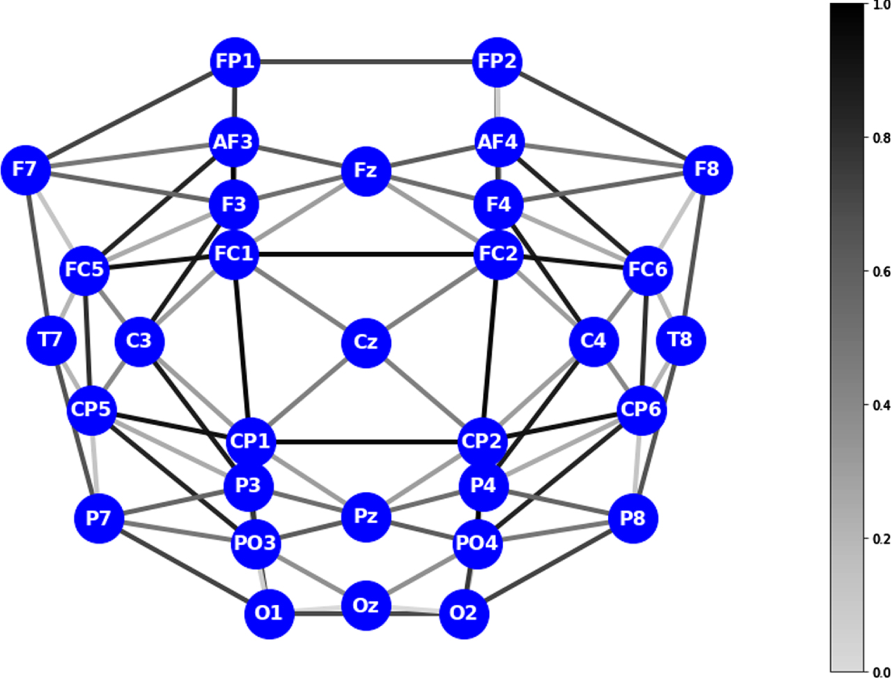
The undirected weighted graph generated at κ = 1.5.

The brain network we have constructed reflects the coupling correlation between two EEG channels. As a result, the network is not highly sensitive to changes in amplitude. This characteristic helps reduce the impact of inter-individual differences on the results, thus facilitating the establishment of a robust and accurate EEG-based recognition model.

3.2 Spectral graph convolution

Spectral graph convolution is an algorithm for processing graph data using neural networks. It combines the concepts of graph theory and neural networks by using graph convolutional operations to model and process graph data, such as Laplace transform and Fourier transform. Graph data is represented as a frequency spectrum matrix, which combines the frequency information of each node with the graph structure information. Then, through convolutional operations on the frequency spectrum matrix, graph features are extracted, and graph Laplace matrix is used to study the properties of the graph. The symmetric normalized Laplace matrix of graph G is defined as follows. $L = E - D^{(- 1 / 2)} W D^{(- 1 / 2)}$ (4) where, E is the unit matrix; $D = diag (d_{1}, . . ., d_{N}) \in ℝ^{N \times N}$ is called the Degree matrix of the graph, herein, $d_{i} = \sum_{j = 1}^{N} W_{ij}$ , that is the number of neighbors of each node; and W is the adjacency matrix.

For a given spatial signal $x \in ℝ^{N \times FN}$ , FN is the characteristic number, and its graph Fourier transform is $\hat{x} = U^{T} x$ (5)

Where $\hat{x}$ is the frequency domain transformed signal; U is the orthogonal matrix obtained by the singular value decomposition of L. The process is as follows $L = U Λ U^{T}$ (6)

The convolution operation for two signals x and y on graph *G is defined as $* G [x, y] = U ((U^{T} x) ⊙ (U^{T} y))$ (7) where, ⊙ is the Hadamard product.

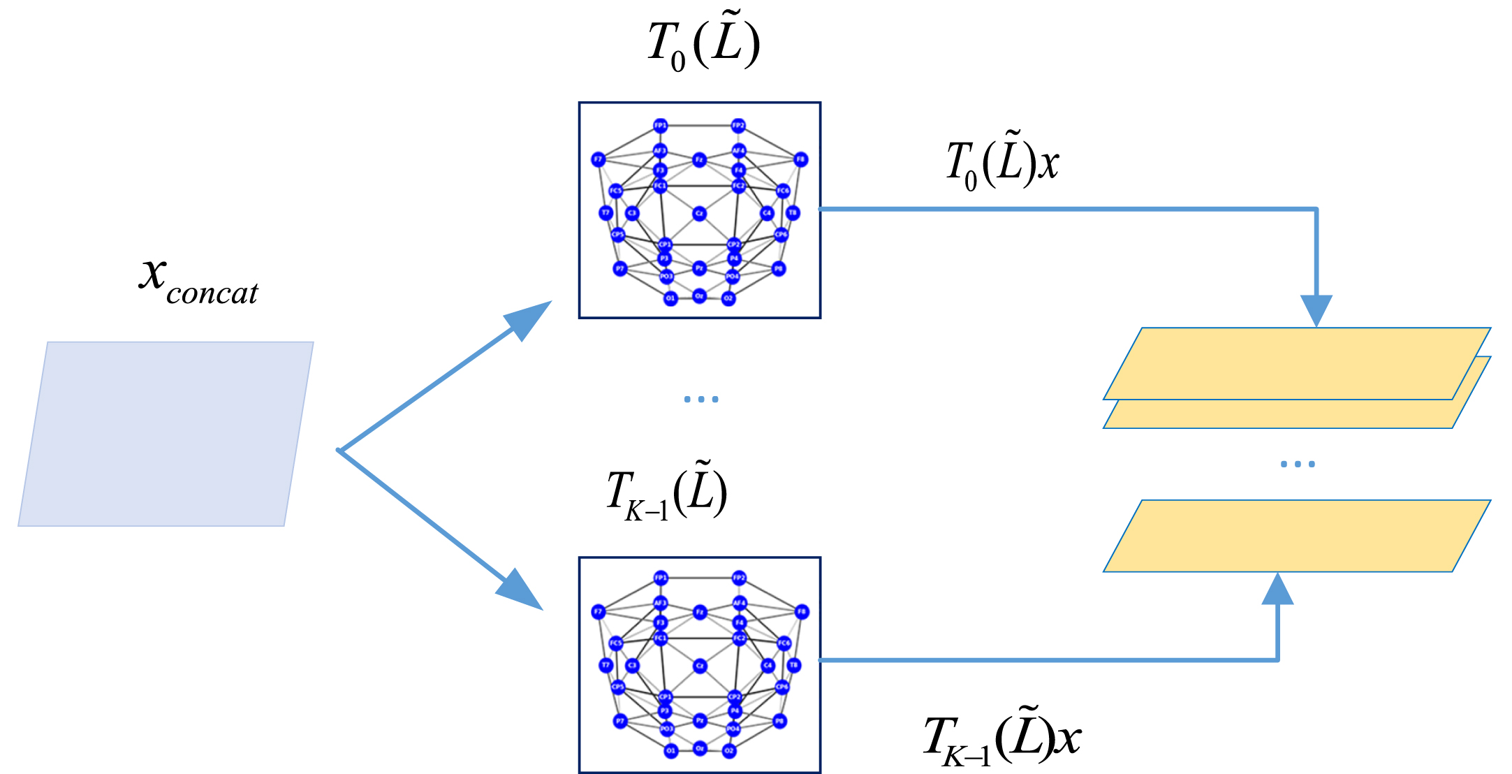
g (·) denotes a filter function, and the signal x filtered by g (L) can be expressed as $y = g (L) x = g (U Λ U^{T}) x = Ug (Λ) U^{T} x$ (8) where, g (Λ) is expressed as follows $g (Λ) = [\begin{matrix} g (λ_{1}) & \dots & 0 \\ ⋮ & ⋱ & ⋮ \\ 0 & \dots & g (λ_{N}) \end{matrix}]$ (9) where, λ₁, λ₂, … , λ_N are the eigenvalues of L.

Since the step of doing the eigendecomposition of L is time-consuming, the K-order Chebyshev polynomial is used instead of the spectral domain convolution kernel, that is the approximation g (Λ), to reduce the parameter complexity. The derivation equation is as follows $g (Λ) = \sum_{k = 0}^{K - 1} θ_{k} T_{k} (\tilde{Λ})$ (10) where, θ_k is the Chebyshev polynomial coefficient and T_k is the calculation of Chebyshev polynomial, which is calculated as follows $T_{0} (x) = 1$ (11) $T_{1} (x) = x$ (12) $T_{k} (x) = 2 x T_{k - 1} (x) - T_{k - 2} (x), k ⩾ 2$ (13)

Combined with equation (8), it can be converted as follows $\begin{matrix} y = Ug (Λ) U^{T} x \\ = \sum_{k = 0}^{K - 1} U [\begin{matrix} θ_{k} T_{k} (λ_{1}) & \dots & 0 \\ ⋮ & ⋱ & ⋮ \\ 0 & \dots & θ_{k} T_{k} (λ_{N}) \end{matrix}] U^{T} x \\ = \sum_{k = 0}^{K - 1} θ_{k} T_{k} (\tilde{L}) x \end{matrix}$ (14) where, $\tilde{L} = \frac{2 L}{λ_{MAX}} - E$ , and E is the unit matrix.

3.3 GRU

GRU is a variant of RNN with a gating mechanism, which is a gated recurrent neural network to better capture the dependencies with larger intervals in the temporal data. Its input contains: input x_t at t, hidden layer state h^t-1 at t - 1, and output structure contains: hidden node output y^t at t, hidden layer state h^t passed to the next node. The process of obtaining the state of reset gate x_t and update gate t - 1 by the state h^t-1 of the previous layer and the current input x_t is as follows. $r_{t} = σ (x_{t} W_{xr} + h^{t - 1} W_{hr} + b_{r})$ (15) $u_{t} = σ (x_{t} W_{xz} + h^{t - 1} W_{hz} + b_{z})$ (16) where, σ is a Sigmoid function that transforms the data to a value in the range of 0 to 1, thus to act as a gating signal.

The candidate hidden layer states are $c_{t} = \tanh (x_{t} W_{hx} + r_{t} ⊙ h^{(t - 1)} W_{hh} + b_{h})$ (17) where, c_t is the candidate hidden state, h^t-1 contains the past information, r_t is the reset gate, and ⊙ is the multiplication by elements.

The final hidden state is $h_{t} = (1 - u_{t}) ⊙ h^{t - 1} + u_{t} ⊙ c_{t}$ (18) where, u_t is the update gate. The past hidden state is combined with the current candidate information by updating the state of the gate to get the result of the final hidden state.

4 SGCRNN for EEG emotion recognition

This section provides a detailed overview of the SGCRNN model for addressing EEG emotion recognition.

4.1 SGCRNN model

Inspired by DCRNN [27], this paper uses a recurrent neural network with spectral graph convolution as an EEG signal sentiment feature extractor to simulate the spatial and temporal dependence of EEG signals. In this paper, ChebNet [28] is employed instead of matrix multiplication in GRU for spatial and temporal modeling of EEG signals (referred to as CNGRU). CNGRU has the advantage of both GRU for extracting temporal correlation and spectral graph convolution for extracting frequency and spatial domain features.

The internal computations of *G are represented as shown in Fig. 2. The input x_concat consists of the concatenation of the input at time t, x_t, and the hidden layer h^t-1 at time t - 1. The output is the result of the Chebnet operation.

Fig. 2

Internal computation representation of “*G”.

The CNGRU network structure is shown in Fig. 3. According to Equations (15)–(18), they can be expressed as follows.

Fig. 3

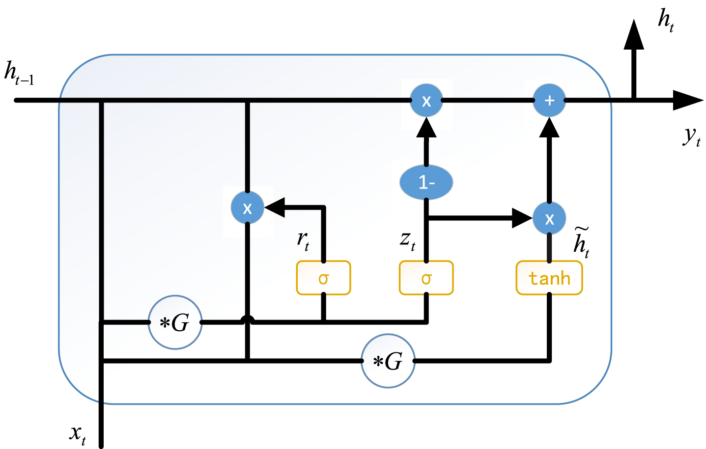
CNGRU network architecture diagram.

$r_{t} = σ (Θ_{r} * G [x_{t}, h_{t - 1}] + b_{r})$ (19) $u_{t} = σ (Θ_{u} * G [x_{t}, h_{t - 1}] + b_{u})$ (20) $c_{t} = tanh (Θ_{c} * G [x_{t}, (r_{r} ⊙ h_{t - 1})] + b_{c})$ (21) $h_{t} = (1 - u_{t}) ⊙ h_{t - 1} + u_{t} ⊙ c_{t}$ (22) where, x_t and h_t denote the input and output of CNGRU at moment t, respectively; σ denotes the Sigmoid function; ⊙ denotes the Hadamard product; r_t, u_t and c_t denote the reset gate, update gate, and candidate gate at moment t, respectively; *G denotes the ChebNet spectral map convolution; Θ_r, b_r, Θ_u, b_u, Θ_c and b_c are the corresponding convolution filters of the weights and biases.

The SGCRNN model consists of two stacked CNGRU layers, a fully connected layer, and a pooling layer for the EEG signal sentiment identification work. The SGCRNN model is shown in Fig. 4. The input section of the model involves handling 32-channel raw EEG signals, each characterized by a specified duration. After applying preprocessing procedures, discrete signals are generated. Subsequently, cosine similarity is employed to construct adjacency matrices for each second, facilitating the creation of a brain network adept at capturing spatial features. It’s important to highlight that the attributes of each node originate from EEG signal feature vector values associated with distinct EEG electrodes.

Fig. 4

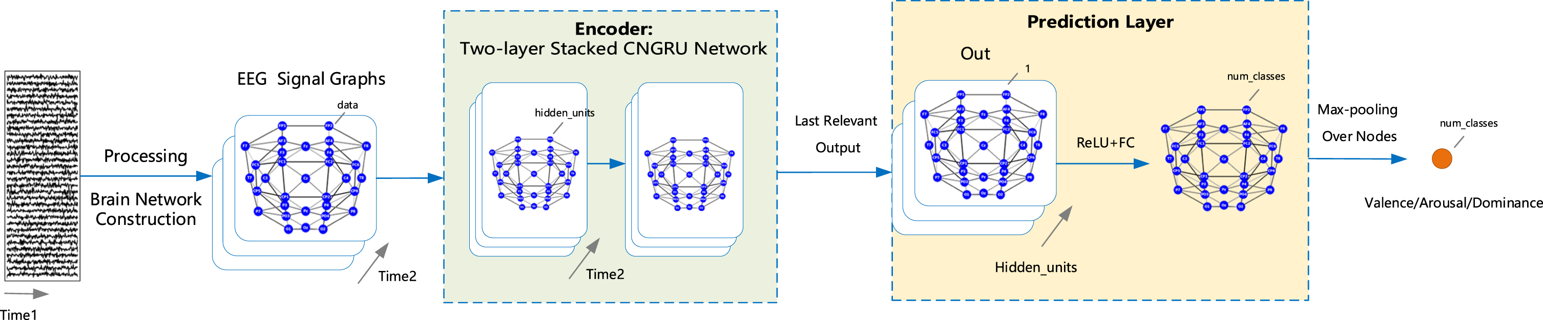
SGCRNN model diagram.

Further insights into the model’s fundamental architecture are established. In this context, a two-layer stacked CNGRU network assumes a pivotal role as the encoder. Sharing similarities with a GRU but featuring enhanced complexities, this network operates through iterative computations executed via time loops. Elaboration on this operational mechanism can be found in Section 4.1, alongside pertinent formulas. Within the encoder module, the “Time2” parameter is set to encompass 12 layers, mirroring the concept of 12 time-based iterations. Consequently, the outputs of the hidden layers adopt a specific structure of (seq_len, hidden_units * num_nodes). For clarity enhancement, topology maps are employed as visual aids, effectively illustrating data formatted as (hidden_units * num_nodes,). Within this visualization, each individual node encapsulates hidden_units data. By leveraging the “Last Relevant Output” component, the model extracts the ultimate pertinent output from the sequence. This output structure takes the form of (num_nodes, hidden_units), thereby delineating the configuration of subsequent “Out” components in terms of hidden_units layers.

The subsequent transition involves the FC layer, employing a Linear function to convert the data into a format denoted as (num_nodes, num_classes). Conclusively, post-processing through a max-pooling layer drives data transformation into the configuration of (num_classes).

In summation, the model adeptly amalgamates spatial aspects of EEG signals with temporal considerations, resulting in an all-encompassing examination of brain networks. This methodology culminates in precise predictions as the model adeptly deciphers intricate patterns and interconnectedness within the brain network.

4.2 SGCRNN algorithm description

In this study, the network parameters are iterated to their optimum values using the backpropagation approach. Therefore, a loss function is defined based on the mean square error, and the SGCRNN model’s loss function is defined as follows. $Loss = mse (p, l) + α | | W | |_{1}$ (23) where, p and l denote the predicted value of the model and the actual label value of the training data, respectively; W denotes all parameters of the model; α denotes the regularization coefficient. The mean square error function mse (p, l) aims to measure the difference between the model prediction and the actual sentiment label value, and the regularization term α||W||₁ aims to prevent the model from overfitting during the parameter learning process.

The SGCRNN algorithm is described in Algorithm 1.

Algorithm 1 SGCRNN description
Input: EEG sample $X \in ℝ^{T \times N \times M}$ data label l, Chebyshev polynomial order K, learning rate λ, maximum number of epochs MAX, early stop patienc ɛ, regularization weight α, number of GRU hidden layer units num_unit, number of CNGRU structures gru_layers;
Output: Ideal parameters for SGCRNN;
1 epoch = 0;
2 while patience< ɛ\|\| epoch < MAX do
3 Reshape input_seq into (T, batch, N, M);
4 Initialize the GRU hidden layer input;
5 fori = 1, . . . ,gru_layers do
6 fori = 1, . . . ,T do
7 Calculate the adjacency matrix according to equation (3);
8 Calculate the symmetrically normalized Laplacian matrix according to equation (4);
9 Calculate the Chebyshev polynomials according to equation (13);
10 Concat x (t) , h^t-1;
11 Calculate the result of spectral graph convolution based on equation (14);
12 Calculate the output of the hidden layer based on equations (22);
13 end
14 end
15 Calculate the output of the FC (Fully Connected) layer;
16 Calculate the output of the Max-pooling layer;
17 Calculate the value of the loss function according to equation (23);
18 Update the model parameters;
19 epoch = epoch+1;
20 end while

5 Experiments and results analysis

5.1 Introduction to data sets

More than 85% of physiological signal emotion recognition studies use the DEAP dataset [29]. The DEAP database [30] is an experimentally gathered multimodal dataset by researchers from Queen Mary University of London in the UK and other institutions to study human emotional states. The researchers recorded EEG and peripheral physiological signals from 32 participants while watching 40 one-minute music videos. Each movie was given a rating from 1 to 9 by participants based on its valence, arousal, like, and dominance.

5.2 Data preprocessing

The 32 channels of labeled EEG signals acquired from this dataset were used for the experiments in this paper, and the data were preprocessed as follows. First, the data were downsampled to 128 Hz, EOG artifacts were removed, and a band-pass frequency filter of 4.0-45.0 Hz was applied to average the data to the same reference. Delete the first three seconds of the baseline signal. In general, the duration of human emotional states is 1 second to 12 seconds. To increase the amount of training data, the 60-second EEG experiment is divided into 12-second time slices. The divided data S = {S₁, S₂, . . . , S_n}, where, S_i ∈ R^M*T, the number of EEG channels M = 32, the number of sampling points T = 1536, and the number of time slices n = 5. Apply the “fft” function from the Scipy python package to each t-second window and retain the logarithmic amplitude of the non-negative frequency components. During the training process, data augmentation can be used by applying random reflections along the scalp midline. This method increases the diversity and randomness of the data by applying random reflections to the EEG sequence and scaling the amplitude of the EEG signal randomly in the range [0.8, 1.2]. This improves the reliability and accuracy of data analysis.

The shape of the data in the dataset is shown in Table 2.

Table 2
Dataset format

Array name Array shape Array contents

Data 6400 × 12 × 32 × 128 samples × seq_lenths × channel × data

Labels 6400 × 3 samples × label (valence, arousal, dominance)

Array name	Array shape	Array contents
Data	6400 × 12 × 32 × 128	samples × seq_lenths × channel × data
Labels	6400 × 3	samples × label (valence, arousal, dominance)

5.3 Evaluation metrics and parameter settings

The prediction accuracy and mean absolute error are used to evaluate the SGCRNN model performance, and they are calculated as follows. $Accuracy = \frac{N_{c}}{N}$ (24) $MAE = \frac{\sum_{i = 1}^{N} | Y_{i} - {\hat{Y}}_{l} |}{N}$ (25) where, N_c is the number of correctly predicted samples, which is defined as the number of samples that satisfy $| Y_{i} - {\hat{Y}}_{l} | ⩽ 2$ ; N is the total number of test sets; Y_i is the dataset label value; ${\hat{Y}}_{l}$ is the model prediction value.

The SGCRNN model consists of two stacked CNGRU layers and 64 hidden units. The Chebyshev polynomial order is set to K = 2, and the number of graph nodes is 32. The activation function is the ReLU activation function. The maximum number of epochs MAX is 300. The dropout probability is 0 (i.e., no dropout). The learning rate η = 1e^(-4). The batch size for the training set is 512, while the batch size for the validation set and test set is 128. The regularization coefficient of the loss function is α = 0.001. The optimizer uses the Adam optimizer. During training, if the loss value after ɛ = 5 epochs is higher than the previous epoch, the training is terminated. CosineAnnealingLR learning rate scheduler is used to train the deep learning model. The scheduler adjusts the learning rate periodically based on the time function of the learning rate. During training, the learning rate gradually decreases with time, achieving better training results. The learning rate curve is shown in Fig. 5. The model was trained and tested on RTX 3090, implemented using Python 3.8.10 and Pytorch 1.11.0. The training set, validation set and test set were divided in the ratio of 8 : 1:1 in the experiments.

Fig. 5

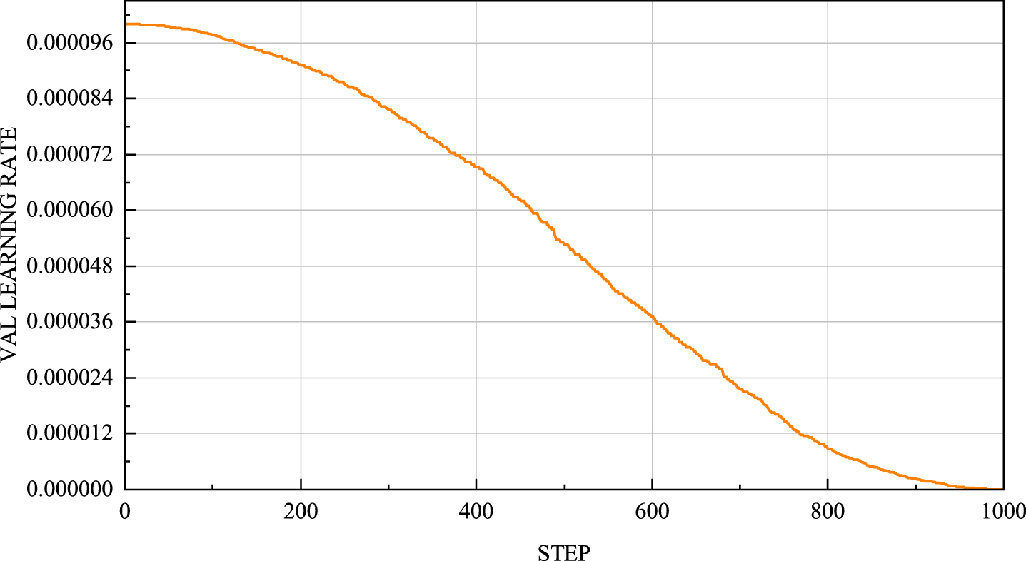
Learning rate scheduler curve.

5.4 Ablation experiments

Ablation experiments are performed in this section to explore the contribution of several important components used in this article to the approach. The first ablation experiment was conducted to verify the effect of the fast Fourier transform, time slice and data enhancement methods used in this paper on the improvement of prediction ability. The second ablation experiment is to test whether the proposed method of establishing the adjacency matrix can further improve the prediction accuracy.

5.4.1 Different ways to process data

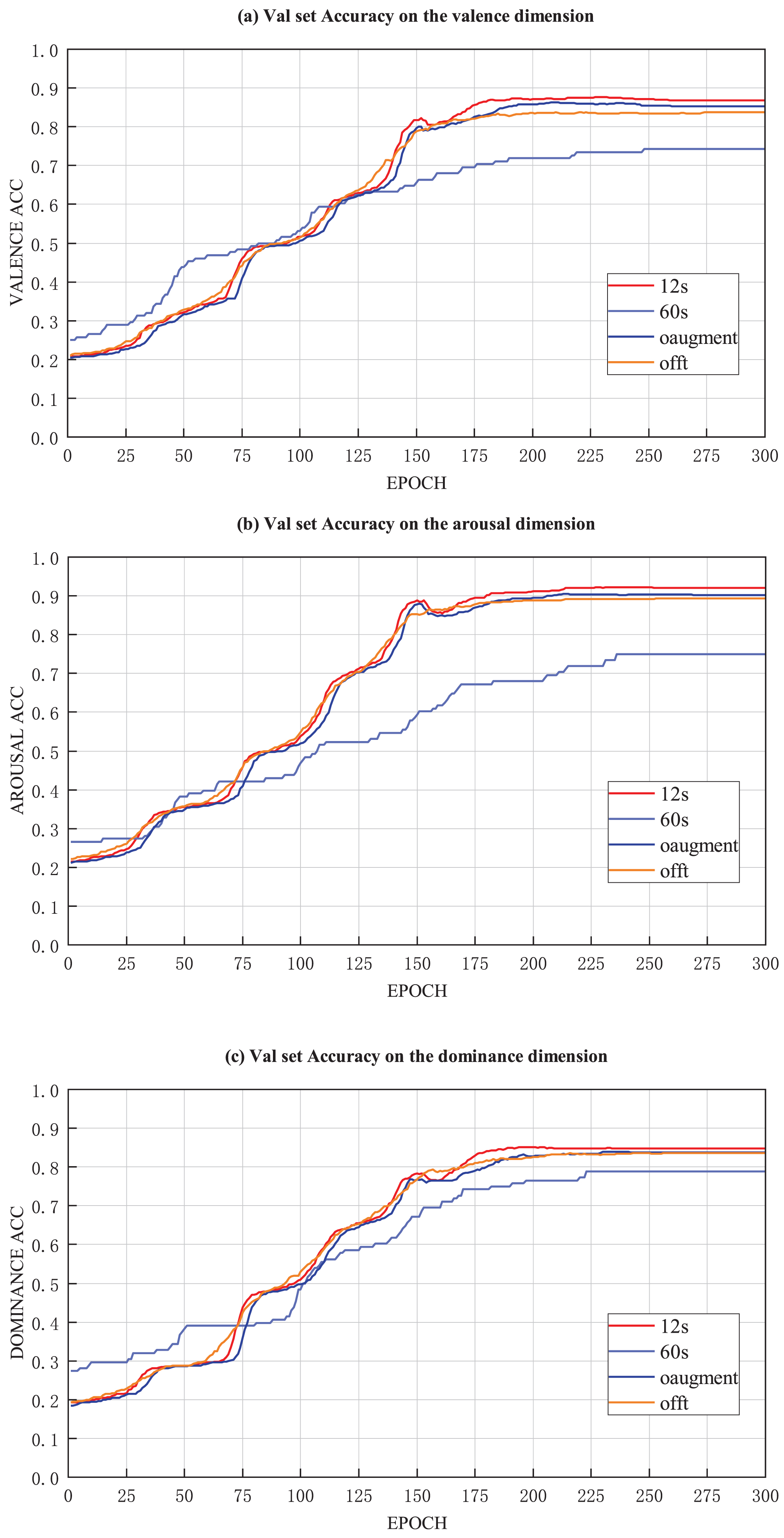
After experimental comparison, this study obtained four sets of data. Experiment 1 directly used time-domain features for training, without FFT; experiment 2 used 60 seconds of data for training, without time slicing; experiment 3 did not perform data augmentation. Experiment 4 used fast Fourier transform and divided the data into 12-second time slices, while also performing data augmentation. We obtained corresponding results through accuracy tests in the three dimensions of valence, arousal, and dominance, as shown in Fig. 6. In addition, the MAE values of various methods have been listed in Fig. 7.

Fig. 6

Accuracy of validation set in three dimensions.

Fig. 7

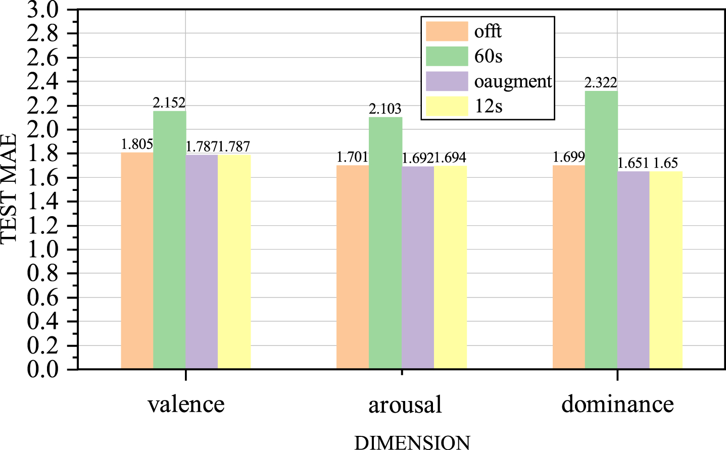
MAE of different methods on the test set.

The three line graphs in Fig. 6 illustrate how the validation set accuracy of the model across three sentiment dimensions changes with an increase in training epochs. They offer a visual understanding of the model’s performance and learning progress. The horizontal axis of the line graphs represents the number of training epochs, while the vertical axis represents the accuracy of the model on the validation set. The accuracy on the validation set serves as a measure of the model’s performance in this sentiment analysis task. A higher accuracy signifies a better match between the model’s predictions and the actual sentiment labels. The bar chart in Fig. 7 provides a summary of the model’s accuracy on the test set for each sentiment dimension, allowing for a quick comparison of the model’s performance across different emotion categories.

Through the comparison of the four experiments mentioned above, it can be observed that the approach used in Experiment 1 had lower accuracy and relatively larger errors in all emotional dimensions, performing worse compared to Experiments 3 and 4. Similarly, Experiment 2’s approach exhibited lower accuracy and larger errors in all emotional dimensions, indicating poorer performance. This suggests that using longer data segments for training is not conducive to improving the accuracy of emotion prediction. On the other hand, Experiment 3’s approach had relatively smaller errors in Valence and Arousal, but slightly larger errors in Dominance. Experiment 4 achieved the highest accuracy and lowest loss values by utilizing techniques such as FFT, time slicing, and data augmentation.

This result indicates that using these technologies can effectively improve the effectiveness of sentiment analysis. Specifically, the fast Fourier transform can convert time-domain signals into frequency-domain signals, thereby better capturing signal characteristics in different frequency ranges. Time slicing can divide long time series into multiple short time periods for processing, avoiding the complexity and difficulty brought by long time series, and better grasping the dynamic changes in instantaneous situations. In addition, using randomly reflected signals along the midline of the scalp can be used for data augmentation, which can extend the dataset, increase the diversity of data, and thus improve the model’s generalization ability. Therefore, the experimental results demonstrate the advantages of the methods used in the data processing process in this paper.

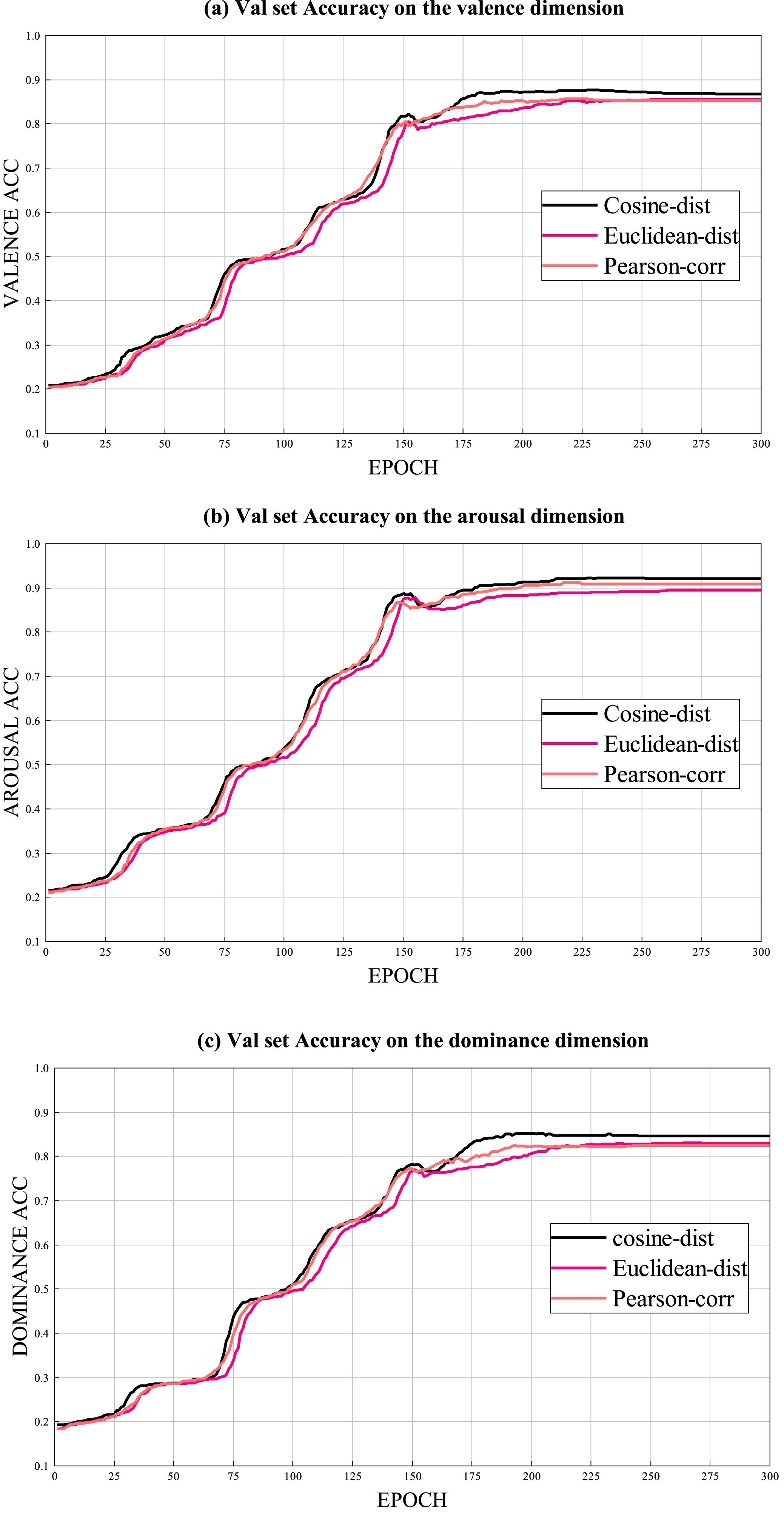
5.4.2 Different ways to build adjacency matrix

The experiment compared three methods for constructing adjacency matrices, including the method based on Euclidean distance of EEG electrode spatial positions, the method based on cosine similarity of EEG electrode spatial positions, and the method based on correlation of EEG channel features. As shown in Fig. 8, the corresponding accuracy results were achieved in three dimensions valence, arousal, and dominance. The MAE values for different methods, as well as the total training time and testing set evaluation time, are shown in Table 3.

Fig. 8

Accuracy of validation set in three dimensions.

Table 3

Test set MAE of different methods

Methods	Valence	Arousal	Dominance	Train Time	Test Time
Euclidean-dist	1.792	1.700	1.668	3.1192h	4s
Pearson-corr	1.794	1.700	1.652	14.7242h	20s
Cosine-dist	1.787	1.694	1.650	2.8892h	3s

The three line graphs in Fig. 8 illustrate the changes in validation set accuracy across three sentiment dimensions as the training epochs progress, considering the variations resulting from different methods used to construct the adjacency matrix.

Method 1 had MAE values of 1.792, 1.700, and 1.668 in the three-dimensional emotional dimensions. The total training time was 3.1192 hours, and the testing set evaluation time was 4 seconds. Method 2 had MAE values of 1.794, 1.700, and 1.652 in the three-dimensional emotional dimensions. The total training time was 14.7242 hours, and the testing set evaluation time was 20 seconds. Method 3 had MAE values of 1.787, 1.694, and 1.650 in the three-dimensional emotional dimensions. The total training time was 2.8892 hours, and the testing set evaluation time was 3 seconds.

Compared to the other two methods, the method of constructing graph adjacency matrix based on cosine similarity of EEG electrode spatial positions shows superiority in training time, accuracy, and loss value. Specifically, the proposed method in this paper has a significantly shorter training duration compared to the other two methods. This will significantly improve training efficiency and reduce the time and energy costs for researchers. Furthermore, in terms of accuracy and loss value, our proposed method outperforms the other two methods, significantly improving the predictive performance and generalization ability of the model. Therefore, our proposed method has high practical value in the application of real-time monitoring.

5.5 Contrastive experiments

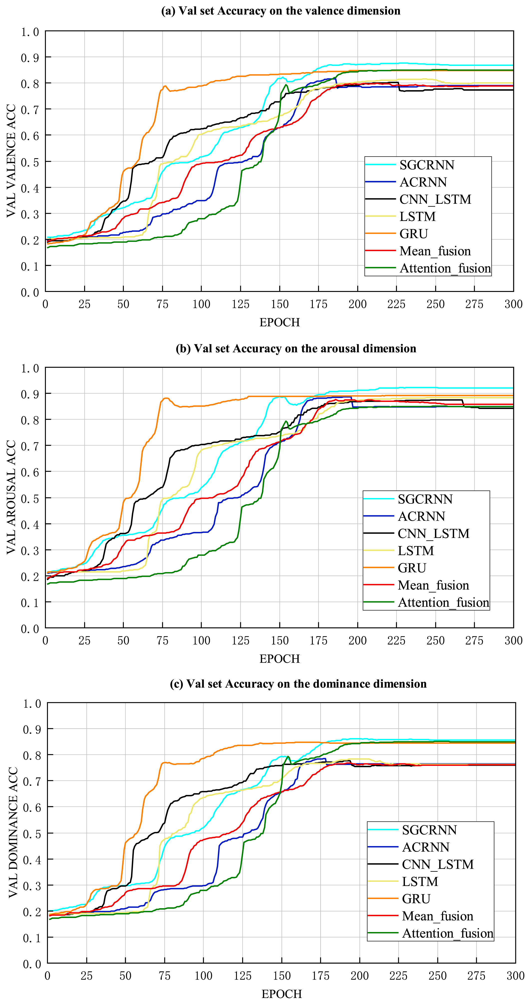
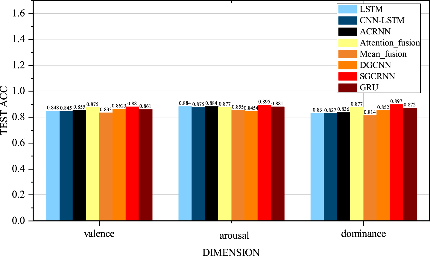
This study evaluated eight EEG emotion recognition models by comparing their prediction accuracy on the validation and test sets. The first model is an Long Short-Term Memory (LSTM) model based on LSTM recurrent neural networks. The second model is a CNN-LSTM model that combines Convolutional Neural Networks with LSTM. The third model is an ACRNN [31] model that combines CNN, LSTM, and attention. The fourth model is a Mean_fusion model that combines the SGCRNN model with the ACRNN model and averages the fusion of EEG signals with peripheral physiological signals. The fifth model is a Attention_fusion model that utilizes attention for multimodal mental signal fusion. The sixth model is a DGCNN [24] model based on Dynamic Graph Convolutional Neural Networks. The seventh model is a GRU model without the ChebNet operation. Additionally, a novel SGCRNN model proposed in this paper is included. All models were trained using the data preprocessing methods proposed earlier. On the validation set, the eight models’ accuracy in predicting Valence, Arousal, and Dominance is shown in Fig. 9, while their prediction accuracy on the test set is shown in Fig. 10.

Fig. 9

Accuracy of validation set in three dimensions.

Fig. 10

MAE of different methods on the test set.

Incorporating Chebyshev polynomials as a replacement for matrix multiplication in the GRU architecture results in a notable enhancement of parameter efficiency for the SGCRNN model. Specifically, the SGCRNN model exhibits a reduced number of trainable parameters, with a total count of 748,562, as opposed to the GRU model which boasts 1,098,817 trainable parameters. This difference underscores the efficacy of our proposed approach in achieving parameter reduction while maintaining model performance. This superiority can be analyzed from two critical perspectives. Firstly, the reduction in trainable parameters contributes to alleviating model complexity, consequently mitigating the risk of overfitting to a certain extent. Secondly, the diminished parameter count translates to reduced computational load and memory requirements, potentially leading to accelerated inference speeds. That is a key advantage, especially in real-time applications.

Moreover, the decrease in trainable parameters does not substantially compromise the performance of the SGCRNN model. Despite the reduced parameter count, the incorporation of Chebyshev polynomials enables the model to preserve its ability to capture spatiotemporal features and handle sequential data, thus ensuring model accuracy and efficacy.

Figure 9 illustrates the changes in validation set accuracy of the model across different sentiment dimensions with an increase in training epochs. The horizontal axis represents the number of training epochs, while the vertical axis represents the accuracy for the corresponding sentiment dimension. As the number of training epochs increases, the curve exhibits different trends and shapes, reflecting the varying learning capacity and convergence of different comparative models. Figure 10 displays the test set accuracy of different models across three sentiment dimensions, using three sets of bar graphs. The horizontal axis represents the sentiment dimensions, while the vertical axis represents the accuracy. Each bar in the bar graphs represents the accuracy of the corresponding model on the respective sentiment dimension.

According to the experimental results above, it can be found that the performance of SGCRNN model exceeds that of other seven methods (LSTM, CNN-LSTM, ACRNN, GRU, Mean_fusion, Attention_fusion, and DGCNN) in all evaluation indicators. In terms of Valence, Arousal, and Dominance, SGCRNN achieved the highest scores of 88%, 89.5%, and 89.7%, respectively. This indicates that SGCRNN has the best effect on emotion recognition of EEG time series.

In terms of convergence speed, this paper conducted an extensive comparison among seven emotion analysis models. Specifically, the SGCRNN model, due to its incorporation of the nonlinear characteristics of Chebyshev networks, captures emotion-related features within EEG signals more rapidly, resulting in a relatively swift convergence trend during the feature learning phase. On the other hand, the fusion of convolutional and recursive operations in the ACRNN model might require more training iterations to achieve stability, thus fully leveraging their role in feature extraction and temporal modeling. Within the CNN_LSTM model, the amalgamation of convolution and LSTM operations might lead to a longer training process, with the aim of better capturing the interaction between temporal and spatial information. Meanwhile, the LSTM model, due to its complex cyclic structure, might exhibit a slightly slower convergence trait when processing time-series data. Significantly, the GRU model, benefiting from its simplified gating mechanism, demonstrates a relatively fast convergence speed when learning long sequence data. In the case of fusion methods, the training speeds of the Mean_fusion and Attention_fusion models are similar, implying a minor influence of fusion strategies on training speed.

Considering both the accuracy results and convergence speeds of the models holistically, this research explicitly demonstrates the superior performance of the SGCRNN model in the task of emotion analysis.

The SGCRNN model uses ChebNet instead of matrix multiplication in GRU, which has the following advantages. Firstly, SGCRNN model can better capture the dynamic evolution of data by combining spatiotemporal dependency, which greatly improves its ability in extracting emotional features from EEG signals. Secondly, the RNN architecture of SGCRNN model can well preserve the sequential relationship of emotion information, inherit the strong sequence learning ability of RNN, and adaptively adjust the parameters of its structure based on feedback mechanism. In conclusion, SGCRNN model is an efficient and accurate method for EEG signal emotion recognition.

6 Conclusions

In this article, we propose a novel SGCRNN model for EEG emotion recognition. Specifically, we first construct a graph adjacency matrix based on the cosine similarity of EEG electrode spatial locations. Then, ChebNet is used to replace matrix multiplication in GRU, resulting in the proposed CNGRU. The EEG sequence is fed into the SGCRNN model, which consists of two stacked CNGRU layers, an FC layer, and a max-pooling layer, to obtain the prediction results. Two ablation experiments and a contrastive experiment were conducted using the DEAP dataset, and the results showed that the data preprocessing methods used in this study, such as using FFT to extract frequency domain features, segmenting time into 12-second slices, and using randomly reflected signals along the scalp for data augmentation, all contribute to improving the model’s accuracy. The novel method proposed in this study to construct the graph adjacency matrix can capture the local relationships between EEG channels and effectively improve training efficiency, outperforming existing methods for constructing adjacency matrices. Moreover, the new SGCRNN model for emotion recognition proposed in this paper can simulate the spatiotemporal dependencies of EEG time series and performs better than other advanced emotion recognition models.

In future research, we will consider the application of real-time emotion recognition and explore how to compress the SGCRNN model for real-time emotion recognition scenarios. Additionally, further research in emotion recognition should focus on addressing individual differences and incorporating them into the emotion recognition model to enhance personalized emotion recognition accuracy and effectiveness. Long-term variations in emotions should also be considered, and models should be developed to capture trends and patterns in long-term emotional changes for long-term emotion recognition and analysis. By delving into these issues, we can strengthen the research and application of emotion recognition based on EEG signals, expanding its potential value in fields such as psychology, medicine, and human-computer interaction.

By combining the expertise of manual engineering with the powerful capabilities of deep learning, we can develop more accurate, efficient, and interpretable emotion recognition systems. These systems can help businesses understand customer emotions and needs, providing personalized products and services. Additionally, they can play a crucial role in psychology and medicine, aiding in the diagnosis and treatment of emotional disorders, as well as monitoring and intervening in emotional states. Through further research and application of these methods, we can explore novel domains and contribute to society with more beneficial solutions.

Footnotes

Acknowledgment

This work is supported by the Science and Technology Development Project in Jilin Province of China (Grantnumbers: 20210402078GH).

References

Horlings

, Datcu

and Rothkrantz

L.J.

, Emotion recognition using brain activity. In Proceedings of the 9th International Conference on Computer Systems and Technologies and Workshop for PhD Students in Computing, (2008), pp. II–1.

Alarcao

S.M.

and Fonseca

M.J.

, Emotions recognition using eeg signals: A survey, IEEE Transactions on Affective Computing 10(3) (2019), 374–393. doi: 10.1109/TAFFC.2017.2714671

Gao

, Lee

H.J.

and Mehmood

R.M.

, Deep learninig of EEG signals for emotion recognition. In 2015 IEEE International Conference on Multimedia & Expo Workshops (ICMEW), (2015), pp. 1–5.https://doi.org/10.1109/ICMEW.2015.7169796

Mehrabian

, Framework for a comprehensive description and measurement of emotional states, Genetic, Social, and General Psychology Monographs (1995).

Russell

J.A.

, A circumplex model of affect, Journal of Personality and Social Psychology 39(6) (1980), 1161.

Chowdary

M.K.

, Anitha

and Hemanth

D.J.

, Emotion recognition from eeg signals using recurrent neural networks, Electronics 11(15) (2022), 2387.

, Guo

and Wang

, Subject-independent EEG emotion recognition with hybrid spatio-temporal GRU-Conv architecture, Medical & Biological Engineering & Computing (2022), 1–13.

Zhong

, Wang

and Miao

, EEG-based emotion recognition using regularized graph neural networks, in IEEE Transactions on Affective Computing 13(3) (2022), 1290–1301, 10.1109/TAFFC.2020.2994159

Yin

, Zheng

, Hu

, Zhang

and Cui

, EEG emotion recognition using fusion model of graph convolutional neural networksand LSTM, Appl. Soft Comput. 100 (2021), 106954. https://doi.org/10.1016/j.asoc.2020.106954

10.

Demir

, Koike-Akino

, Wang

, Haruna

and Erdogmus

, EEG-GNN: graph neural networks for classification of electroencephalogram (EEG) signals, Annu Int Conf IEEE Eng Med Biol Soc. 2021 (2021), 1061–1067. doi: 10.1109/EMBC46164.2021.9630194. PMID: 34891471

11.

Ed Bullmore and Olaf Sporns , The economy of brain network organization, Nature Reviews Neuroscience 13(5) (2012), 336–349.

12.

Richard Betzel

and Danielle Bassett

, Multi-scale brain networks, Neuroimage 160 (2017), 73–83.

13.

Jia

, Zhang

, Lv

, Xu

, Hu

and Li

, CR-GCN: channel-relationships-based graph convolutional network for EEG emotion recognition, Brain Sciences 12(8) (2022), 987.

14.

Chen

, Feng

, Jiang

and Zhu

, State of charge estimation of lithium-ion battery using denoising autoencoder and gated recurrent unit recurrent neural network, Energy 227 (2021), 120451.

15.

Tripathi

, Acharya

, Sharma

R.D.

, Mittal

and Bhattacharya

, Using deep and convolutional neural networks for accurate emotion classification on deap dataset. In Proceedings of the 29th IAAI Conference, San Francisco, CA, USA, 4–9 February 2017.

16.

Yang

, Han

and Min

, A multi-column CNN model for emotion recognition from EEG signals, Sensors 19(21) (2019), 4736. https://doi.org/10.3390/s19214736

17.

Liao

, Zhong

, Zhu

and Cai

, Multimodal physiological signal emotion recognition based on convolutional recurrent neural network. In IOP Conference Series: Materials Science and Engineering (Vol. 782, No. 3, (2020) p. 032005). IOP Publishing.

18.

Salama

E.S.

, El-Khoribi

R.A.

, Shoman

M.E.

and Shalaby

M.A.W.

, A 3D-convolutional neural network framework with ensemble learning techniques for multi-modal emotion recognition, Egyptian Informatics Journal 22(2) (2021), 167–176. https://doi.org/10.1016/j.eij.2020.07.005

19.

Cui

, Xuan

, Liu

, et al. Emotion Recognition on EEG Signal Using ResNeXt Attention 2D-3D Convolution Neural Networks, Neural Process Lett (2022). https://doi.org/10.1007/s11063-022-11120-0

20.

Iyer

, Das

S.S.

, Teotia

, et al. CNN and LSTM based ensemble learning for human emotion recognition using EEG recordings, Multimed Tools Appl 82 (2023), 4883–4896. https://doi.org/10.1007/s11042-022-12310-7

21.

Kim

G.I.

and Jang

, Petroleum Price Prediction with CNN-LSTM and CNN-GRU Using Skip-Connection, Mathematics 11 (2023), 547. https://doi.org/10.3390/math11030547

22.

Wang

, Zhang

, Xu

, Chen

, Xing

and Chen

C.L.P.

Eeg emotion recognition using dynamical graph convolutional neural networks and broad learning system, in: 2018 IEEE International Conference on Bioinformatics and Biomedicine (BIBM), 2018, pp. 1240–1244. 10.1109/bibm.2018. 8621147.

23.

Zhong

, Wang

and Miao

, EEG-based emotion recognition using regularized graph neural networks, IEEE Transactions on Affective Computing (2020).

24.

Song

, Zheng

, Song

and Cui

, EEG emotion recognition using dynamical graph convolutional neural networks, IEEE Transactions on Affective Computing 11(3) (2018), 532–541.

25.

Casson

A.J.

, Yates

D.C.

, Smith

S.J.

, Duncan

J.S.

and Rodriguez-Villegas

, Wearable electroencephalography, IEEE Engineering in Medicine and Biology Magazine 29(3) (2010), 44–56. https://doi.org/10.1109/MEMB.2010.936545

26.

Bashivan

, Rish

and Heisig

, Mental state recognition via wearable EEG. arXiv preprint arXiv:1602.00985 (2016).

27.

Mallick

, Balaprakash

, Rask

and Macfarlane

, Graph-partitioning-based diffusion convolutional recurrent neural network for large-scale traffic forecasting, Transportation Research Record 2674(9) (2020), 473–488. https://doi.org/10.1177/0361198120930010

28.

Defferrard

, Bresson

and Vandergheynst

, Convolutional Neural Networks on Graphs with Fast Localized Spectral Filtering. (2016), 10.48550/arXiv.1606.09375.

29.

Abdulrahman

and Baykara

, A comprehensive review for emotion detection based on EEG signals: Challenges, applications, and open issues, Traitement du Signal 38(4) (2021), 1189–1200. https://doi.org/10.18280/ts.380430

30.

Koelstra

, Muhl

, Soleymani

, Lee

J.S.

, Yazdani

, Ebrahimi

and Patras

, Deap: A database for emotion analysis; using physiological signals, IEEE Transactions on Affective Computing 3(1) (2011), 18–31.

31.

Tao

, et al., “EEG-Based Emotion Recognition via Channel-Wise Attention and Self Attention,”, in IEEE Transactions on Affective Computing 14(1) (2023), 382–393, doi: 10.1109/TAFFC.2020.3025777

SGCRNN: A ChebNet-GRU fusion model for eeg emotion recognition

Abstract

Keywords

1 Introduction

2 Related work

2.1 Feature extraction

3 Graph-based EEGs modeling

3.1 Brain network construction

4.1 SGCRNN model

5.1 Introduction to data sets

5.2 Data preprocessing

Table 2 Dataset format Array name Array shape Array contents Data 6400 × 12 × 32 × 128 samples × seqlenths × channel × data Labels 6400 × 3 samples × label (valence, arousal, dominance)

5.4.1 Different ways to process data

Footnotes

Acknowledgment

References

Table 2
Dataset format

Array name Array shape Array contents

Data 6400 × 12 × 32 × 128 samples × seq_lenths × channel × data

Labels 6400 × 3 samples × label (valence, arousal, dominance)